Wind speed forecasting using neural networks

Abstract

The prediction of wind speed is critical in the assessment of feasibility of a potential wind turbine site. This work presents a study on prediction of wind speed using artificial neural networks. Two variations of artificial neural networks, namely, nonlinear autoregressive neural network and nonlinear autoregressive neural network with exogenous inputs, were used to predict wind speed utilizing 1 year of hourly weather data from four locations around the United States to train, validate, and test these networks. This study optimized both neural network configurations and it demonstrated that both models were suitable for wind speed prediction. Both models outperformed persistence model (with a factor of about 2 to 10 in root mean square error ratio). Both artificial neural network models were implemented for single-step and multi-step-ahead prediction of wind speed for all four locations and results were compared. Nonlinear autoregressive neural network with exogenous inputs model gave better prediction performance than nonlinear autoregressive model and the difference was statistically significant.

Keywords

Artificial neural network forecasting multi-step-ahead prediction nonlinear autoregressive networks nonlinear autoregressive neural network with exogenous inputs networks single-step-ahead prediction time series prediction wind speed prediction wind energy site selection

Introduction

Wind energy has become the world’s fastest growing renewable energy source due to its environment friendliness and economic viability. However, due to various conditions at locations for wind energy power generation, accurate information of the dynamic nature of turbines and the wind that drives these wind turbines is needed for wind farm siting, as well as operations and management of the wind energy conversion systems. Wind energy conversion has been known to be a successful technique in order to generate power, particularly for isolated regions. Studies and practice have shown that it is greatly beneficial to forecast wind speed, and thus wind power, for the optimal operation of a wind turbine that has significant wind activity and penetration. An accurate forecast of wind speed allows a balance between maximizing reliability and minimizing operating costs. Wind speed is considered one of the most difficult meteorological parameters to forecast because of the interactions among other prominent weather forces such as temperature and pressure differences, topological surface conditions, as well as the Earth’s rotation. Wind forecasting in the order of seconds to minutes is normally applicable to the control of a wind turbine. Forecasting in the order of hours addresses the problem of scheduling with a power system. Forecasts that predict in the range of days address the problem of maintenance and resource planning. In order to meet the US Department of Energy projected target of 35% of US energy coming from wind by 2035 (US Department of Energy, 2015), there is a strong need to consider forecasting of wind speed at potential wind energy sites for exploration and greater penetration.

Wind speed prediction and forecasting are representative of a time series regression (Berge, 2002; Brand and Kok, 2002; Camara et al., 2016; Cao et al., 2012; Doucoure et al., 2016; Fadare, 2010; Haydari et al., 2007; Jursa, 2007; Kaminsky et al., 1985; Kariniotakis et al., 1996; Kiartzis et al., 1995; Lei et al., 2009; Macas et al., 2016; Milligan et al., 2003; More and Deo, 2003; Nagy, 2016; Sanchez, 2008; Sfetsos, 2000; Tande and Landberg, 1993; Torres et al., 2005; Welch et al., 2009; Yu et al., 2006). Nagy (2016) proposed a generalized additive tree ensemble method in order to predict wind power generation along with solar power generation. Camara et al. (2016) used autoregressive moving average model (ARIMA) with neural network models to predict energy consumption. Torres et al. (2005) used the ARIMA model to predict hourly average wind speeds. Doucoure et al. (2016) employed artificial wavelet neural network and multi-resolution analysis to determine time series predictions using wind speed data. Haydari et al. (2007) presented a time series electric load prediction model using neuro-fuzzy techniques.

There have been a number of studies that have reported very good results and success in real-world applications of using artificial neural networks (ANNs) (Doucoure et al., 2016; Jursa, 2007; Kiartzis et al., 1995; Macas et al., 2016; Sanchez, 2008). Experiments comparing ANNs to other techniques have shown that ANNs have often yielded superior outcomes (Brand and Kok, 2002; Fadare, 2010; Kariniotakis et al., 1996; More and Deo, 2003; Tande and Landberg, 1993). A reason that ANNs outperform other techniques is the capability of ANN in modeling nonlinear data sets (Cigizoglu and Kisi, 2005; Samanta, 2004, 2011). In addition, ANNs, once trained, are effective in prediction with acceptable performance. Welch et al. (2009) compared a feedforward and feedback neural network design for short-term wind speed prediction. Sfetsos (2000) compared a variety of forecasting techniques including ANNs for mean hourly wind speed time series.

Recurrent neural networks (RNNs), as well as nonlinear autoregressive (NAR) and nonlinear autoregressive neural networks with exogenous inputs (NARX) networks, can prove useful in predicting nonlinear system data (Cao et al., 2012; Mohanty et al., 2015). These ANNs can use time series data as dynamic input sets. NAR networks use past data in the time series, while RNNs do not as the latter has recurrent connections in its architecture.

This study is concerned with using NAR and NARX methods in order to predict wind speed. The objective of this study is to use a methodology that would optimize these two neural networks for the problem at hand and examine the effectiveness of these ANNs for wind speed prediction. This study then determines if external data can be used to improve performance. One year of hourly weather data was used from four locations around the United States in order to train, optimize, validate, and test these networks.

The rest of the article is organized as follows. In section “Data sets,” data sets of wind speed and other weather parameters used for the study are presented. It is followed with the presentation of details of two ANN models, namely, NAR and NARX, for wind speed prediction. In section “Results and discussion,” results of optimization, training, validation and test of ANNs are presented along with detailed discussions on comparison of prediction performances of the ANNs. Finally, this article concludes summarizing the salient features of this study and outlines future scope of work.

Data sets

The wind speed prediction required data sets of hourly average wind speed and dry bulb temperature readings over a year’s time at multiple locations. Historical weather data from Savannah International Airport (GA), the Bismarck Municipal Airport (ND), Logan International Airport (MA), and the John F. Kennedy International Airport (NY) were obtained through the National Climatic Data Center (NCDC) climate data online (National Oceanic and Atmospheric Administration (NOAA) National Centers for Environmental Information, 2010). The data included hourly mean wind speed in mile/h and hourly dry bulb temperature in degrees Fahrenheit from 1 January 2010 to 31 December 2010. The latter three airports are considered to have some of the worst year round weather according to the NCDC. The data were normalized to be in a range between 0 and 1 in order to compare results for different data sets and prevent local maxima/minima from skewing results. The data were normalized using equation (1). A sample set of the normalized data from Logan International Airport in Boston, MA, is presented in Figure 1

z_{i} = \frac{x_{i} - \min (x)}{\max (x) - \min (x)}

(1)

Figure 1.

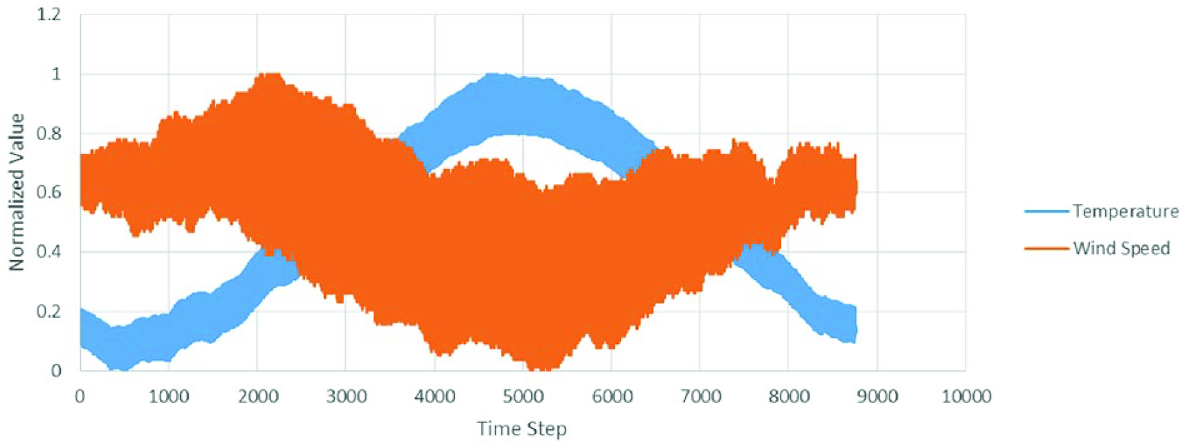
Temperature and wind speed time series over 1 h time steps (normalized) Boston data set (National Oceanic and Atmospheric Administration (NOAA) National Centers for Environmental Information, 2010).

Seventy percent of the data were used for training with Levenberg–Marquardt back propagation (LMBP) (Marquardt, 1963) learning algorithm of MATLAB ANN toolbox (Hagan et al., 1996; Mathworks, 2017). Fifteen percent of the data were used for validation. Validation is used to measure network generalization and to stop the training when generalization does not improve any more. Generalization stops improving as indicated by an increase in the mean square error (MSE) of the validation samples. The remaining 15% was used as testing data. Testing has no effect on the training phase and is used to independently evaluate the network performance after training.

Wind speed prediction

The process of wind speed prediction was done in three stages: first, the data were collected and pre-processed; next, ANN models (NAR and NARX) were implemented within MATLAB neural network toolbox; and finally, the performance of ANN models was analyzed and compared.

NAR and NARX both have pros and cons: the NAR methods are simpler than NARX and require less data. NARX methods allow the use of more information that corresponds to the data set to be predicted. In a wind power generation application, meteorological towers at the site should generate wind speed data as well as other corresponding weather data such as ambient pressure and temperature. The next subsections describe each model and how it can solve the issue of wind speed time series regression.

NAR model

In most applications, time series problems have a high degree of transient periods as well as great variation or disparity. This is why most time series problems are difficult to approximate using a linear model and a nonlinear approach is recommended. An NAR neural network (Jursa, 2007; Mohanty et al., 2015) that is used for a time series regression problem describes a discrete, nonlinear, autoregressive model that can be expressed in equation (2)

y (t) = f (y (t - 1), \dots, y (t - d))

(2)

Equation (2) defines how NAR methods are used to predict the value of a data series y at the time t, y(t) using d past values of the time series. The function f(∙) is not known prior to training. During the training stage, the ANN tries to determine optimal weights and neuron biases in order to approximate the function.

The topology of an NAR network can be seen in Figure 2. The d features $(y (t - 1), \dots, y (t - d))$ are called feedback delays, shown as 1:28 (for d = 28). The hidden layer is characterized by the number of neurons (s), the weight matrix ( W of size $s \times d$ ), the bias vector ( b of size $s \times 1$ ), and the activation function (shown as the nonlinear function symbol for the hidden layer and the linear function symbol for the output layer) for each of s neurons. The number of neurons in a layer is shown below the layer (s = 3 for the hidden layer and 1 for the output layer). The number of feedback delays and neurons per hidden layer are optimized through trial-and-error testing in order to obtain the network architecture for the best performance. It must be noted that increasing the number of neurons in the hidden layer makes a system more complex and decreasing the number of neurons in the hidden layer will lower the computing load at the cost of lower generalization capability of the ANN.

Figure 2.

Neural network setup for an open nonlinear autoregressive (NAR) time series problem.

The learning rule used for NAR networks is the LMBP (Hagan et al., 1996; Marquardt, 1963; Mathworks, 2017). LMBP is used to calculate the second-order derivative without having to calculate the Hessian matrix. The performance function is in the form of a sum of squares of difference between the actual and the predicted values. This performance function allows the Hessian matrix to be calculated (equation (3)) and the gradient can be approximated (equation (4))

H = J^{T} J

(3)

g = J^{T} e

(4)

In equations (3) and (4), J is the Jacobian matrix. The Jacobian matrix has the first derivatives of the network error with respect to the weights and the biases. The variable e is a vector of the network errors in every training sample. In order to approximate the Jacobian matrix, the study by Cigizoglu and Kisi (2005) uses the typical backpropagation method to estimate the Hessian matrix. The Levenberg–Marquardt method uses the following approach to approximate the Hessian matrix (equation (5))

x_{k + 1} = x_{k} - {[J^{T} J + μ I]}^{- 1} J^{T} e

(5)

The method used in this ANN assumes that the performance function is sum of squares such as MSE or error sum of squares (SSE) as stated in equations (6) and (7). In these two equations $y_{i}$ stands for the ith data sample, ${\hat{y}}_{i}$ represents the data that was approximated by the network for $y_{i}$ , and n represents the number of data samples for the network training

S S E = \sum_{i = 1}^{n} {({\hat{y}}_{i} - y_{i})}^{2}

(6)

M S E = \frac{S S E}{n}

(7)

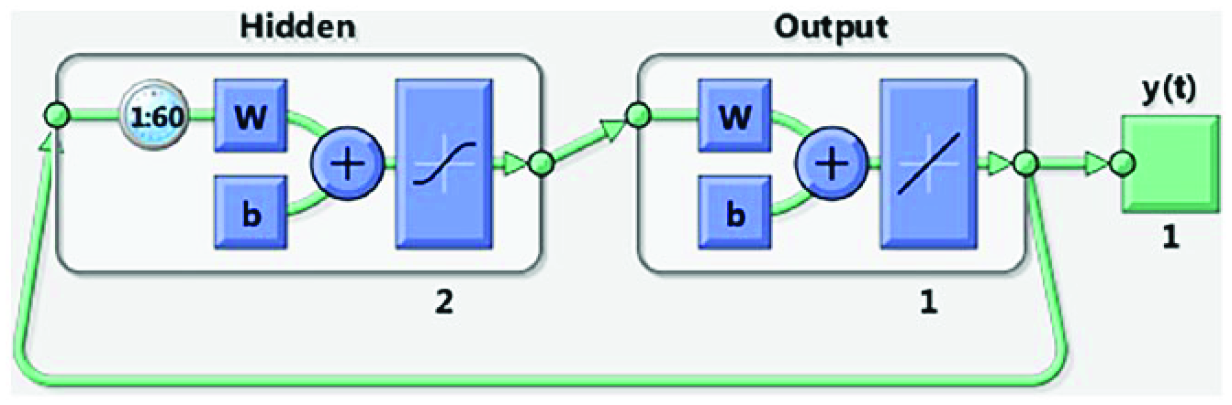
In this study, the NAR method is used to model a wind speed time series regression problem and is planned as such: the network architecture receives one input (corresponding to the wind speed at time t – 1, y(t – 1)) and one output (the following value of the series, y(t), to be predicted). The number of delays and hidden neurons to be used is determined experimentally after data are normalized and analyzed.

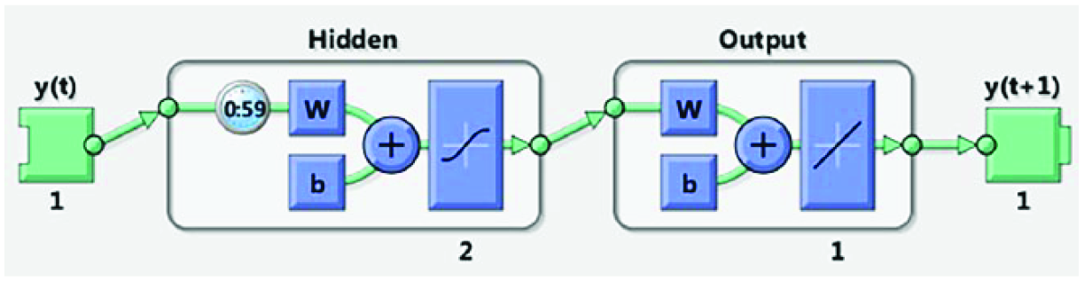
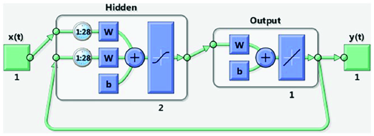
After an optimized NAR architecture has been established, the performance of single-step-ahead prediction (Figure 3) and multi-step-ahead prediction using a closed-loop network (Figure 4) is evaluated. A single-step-ahead prediction network is created by removing one delay tap so that its minimal delay tap is now 0 instead of 1. The new network returns the same outputs as the original network, but outputs are shifted one time step. A closed-loop network is created by replacing the feedback input with a direct connection from the output layer. When using multi-step prediction, the network is simulated in open-loop form for as long as there is known output data, then it is switched to closed-loop form to perform multi-step prediction while providing only the external input. In this study, all but five time steps of the input series and target series (of hourly wind speed) are used to simulate the network in open-loop form. This produces a forecast 5 h ahead of the most recent data collection point.

Figure 3.

Neural network setup for an open-loop nonlinear autoregressive (NAR) time series problem for single-step-ahead prediction.

Figure 4.

Neural network setup for a closed-loop nonlinear autoregressive (NAR) time series problem for multi-step-ahead prediction.

NARX model

In many applications, time series have important correlations between the time series to be modeled and additional exogenous data. It is known that wind speed is highly correlated with both ambient temperature and pressure (Berge, 2002; Kaminsky et al., 1985). The use of these additional weather data sets could benefit forecasting of wind speed in order to provide a more accurate prediction (Yu et al., 2006).

NARX is the other model used in this study. NARX methods predict the time series y(t) given past d values of series y and another external input series x(t), which can be single or multidimensional inputs. Equation (8) models the NARX model for regressive time series forecasting

y (t) = f (x (t - 1), \dots, x (t - d), y (t - 1), \dots, y (t - d))

(8)

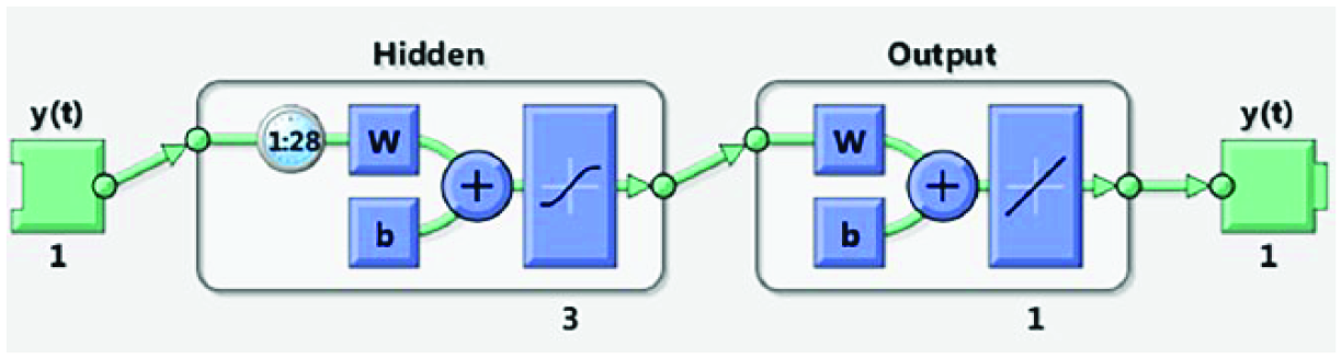
The NARX is a nonlinear model that approximates time step ahead values of a time series based on previous outputs and external data. This study uses one input for the wind speed time series at time t – 1, y(t – 1), and an additional external input of dry bulb temperature at time t – 1, x(t – 1) to produce a single output y(t) that corresponds to the value of the wind speed at one time step (1 h) forward. Figure 5 shows the topology for the NARX network. The learning rule used in training is still the LMBP as explained in the previous section or NAR models.

Figure 5.

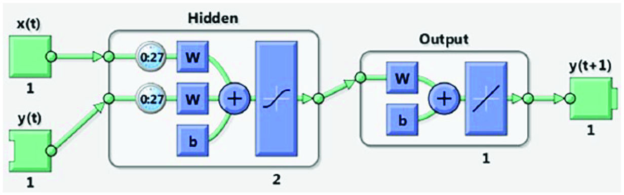
Neural network setup for an open-loop nonlinear autoregressive (NARX) time series problem for single-step-ahead prediction.

After an optimized NARX architecture is established, the performance of single-step-ahead prediction (Figure 5) and multi-step-ahead prediction using a closed-loop network (Figure 6) is evaluated. Both these NARX networks are shown with optimized tapped delay (d = 28) and number of hidden neurons (s = 6). Figures 5 and 6 are counterparts of NAR models (Figures 3 and 4) corresponding to single- and multi-step-ahead time series prediction, respectively.

Figure 6.

Neural network setup for a closed-loop nonlinear autoregressive (NARX) time series problem for multi-step-ahead prediction.

Results and discussion

Figure 7 presents the wind data (National Oceanic and Atmospheric Administration (NOAA) National Centers for Environmental Information, 2010) used in the study, but the time steps have been increased to every 48 h to produce a plot with greater legibility. Noting the shape of the curves, the Logan International Airport (Boston) and JFK airport (JFK) seem to have higher variability and overall higher wind speeds while Bismarck Municipal Airport (BNDA) and Savannah International Airport (SIA) seem to have less variability and overall lower wind speeds.

Figure 7.

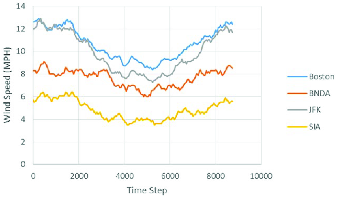
Average hourly wind speed data for the four different airports used in the study displayed as time steps of every 48 h for legibility (Kaminsky et al., 1985).

Optimization of the network architecture

Data sets do not have a relationship between each other due to their geographical locations. This is why it was important to adjust the delay parameters for each data set individually. Delay parameters concern the number of hours the ANN will use to execute the prediction. Put simply, the model is trained with the last d time-steps as delays. Eighteen different tests were conducted on each data set in order to determine the optimal number of delays. The delay values included d = 2, d = 4, d = 8; the last 12 h: d = 12, d = 16, d = 20; the last day: d = 24 and d = 36; the last 2 days: d = 48 and d = 60; and the last 3 days: d = 72. To find the best delay, all the parameters were set to a fixed value (hidden neurons set at 10) and the delays were modified in a trial and error procedure in order to optimize network structure and performance.

Table 1 shows the average MSE of 10 runs for each delay value and location, using the NAR model. The best delay values are marked in bold; for all data sets, two delays resulted in the minimum error. The minimum number of delays in order to get the lowest error was 48 h for the Bismarck Municipal (BNDA) data set while the best delay was 72 h for the JFK data set, the other two data sets had the minimum error at d = 60. From this information, it can be determined that a delay parameter between 48 and 72 previous hours is needed in order to obtain an accurate model.

Table 1.

MSE of the delay parameter obtained with the NAR model (bold values: best delay).

NAR delays
Data set	2	3	4	6	8	10	12	14	16
Boston	1.21E–03	1.09E–03	1.03E–03	1.08E–03	1.00E–03	8.83E–04	9.94E–04	9.14E–04	8.22E–04
BNDA	1.22E–03	1.13E–03	1.25E–03	1.33E–03	1.44E–03	1.54E–03	1.69E–03	1.60E–03	1.98E–03
JFK	1.33E–03	1.13E–03	1.08E–03	1.24E–03	1.21E–03	1.14E–03	1.28E–03	1.55E–03	9.86E–04
SIA	1.29E–03	1.20E–03	1.04E–03	1.18E–03	1.95E–03	2.04E–03	2.29E–03	1.50E–03	1.76E–03
Mean	1.26E–03	1.14E–03	1.10E–03	1.21E–03	1.40E–03	1.40E–03	1.57E–03	1.39E–03	1.39E–03
Data set	18	20	24	26	28	36	48	60	72
Boston	5.52E–04	5.46E–04	1.50E–04	7.46E–05	7.29E–05	7.10E–05	7.12E–05	6.93E–05	7.05E–05
BNDA	1.34E–03	1.03E–03	1.33E–04	6.36E–05	6.49E–05	6.52E–05	6.33E–05	6.68E–05	6.37E–05
JFK	8.97E–04	9.33E–04	1.29E–04	6.42E–05	6.39E–05	6.15E–05	6.44E–05	5.90E–05	5.87E–05
SIA	1.22E–03	7.75E–04	1.58E–04	6.26E–05	6.31E–05	6.35E–05	6.64E–05	5.98E–05	6.22E–05
Mean	1.00E–03	8.20E–04	1.42E–04	6.63E–05	6.62E–05	6.53E–05	6.63E–05	6.37E–05	6.38E–05

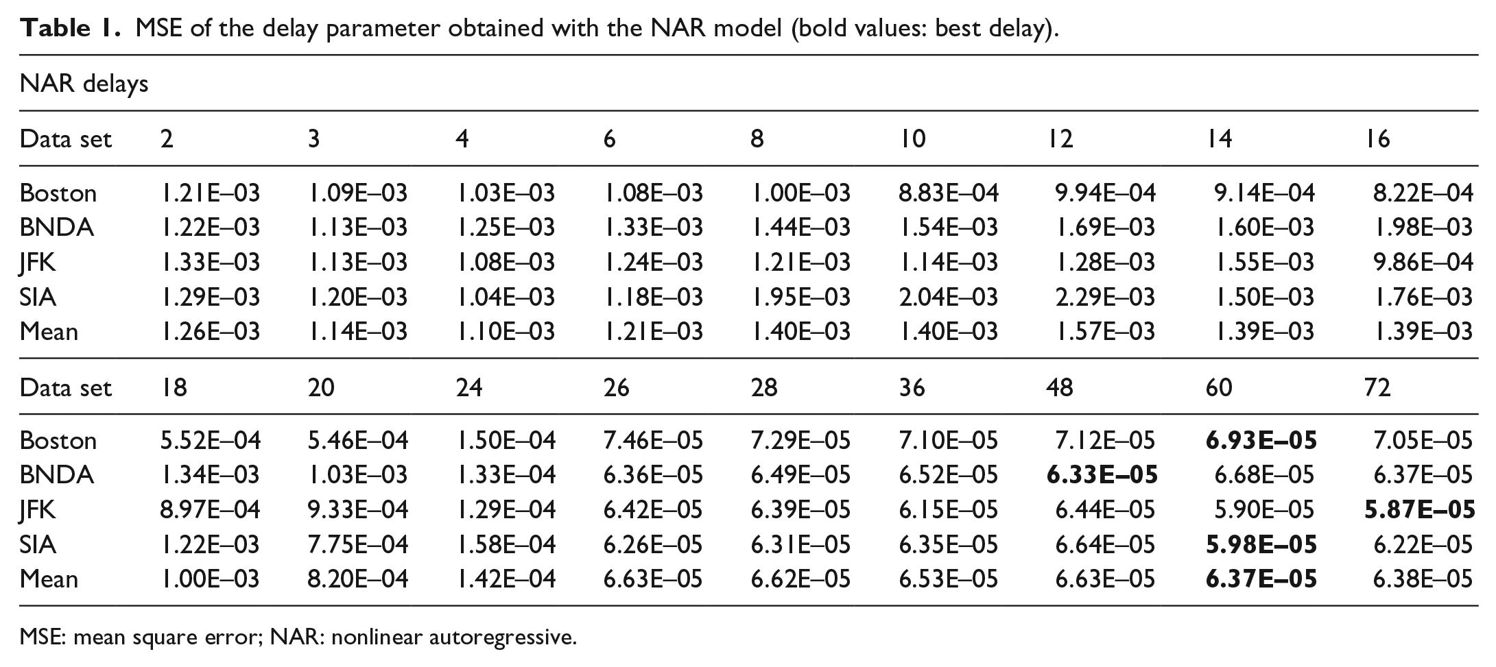
MSE: mean square error; NAR: nonlinear autoregressive.

Once the optimal number of delays has been determined for a data set, the number of hidden layer neurons was found with the corresponding optimal number of delays. With the fixed delay value determined from each data set’s lowest MSE value, 10 different runs for each neuron count were conducted and the average MSE of each setting was calculated. Table 2 shows results with different number of hidden layer neurons ranging from 2 to 20. The purpose of this experiment was to determine which network architecture could provide the lowest error and therefore best performance. It was found that as the neuron count was increased, the prediction was worse due to local minima using the LMBP learning algorithm, as well as overtraining. From Table 2, it can be concluded that the best average MSE values occur at either two or three neurons in the hidden layer, depending on which location was being tested.

Table 2.

MSE of the hidden neurons parameter obtained with the NAR model (bold values: best neuron count).

Number of hidden layer neurons for NAR
Data set	2	3	4	6	8	10	12	14	16	18	20
Boston	6.91E–05	5.81E–05	7.11E–05	7.22E–05	7.59E–05	7.37E–05	7.66E–05	7.48E–05	7.95E–05	7.94E–05	8.38E–05
BNDA	5.88E–05	6.01E–05	6.16E–05	6.43E–05	6.73E–05	6.76E–05	7.81E–05	7.36E–05	7.98E–05	8.02E–05	8.35E–05
JFK	5.84E–05	6.22E–05	5.85E–05	6.21E–05	6.06E–05	6.06E–05	6.82E–05	7.46E–05	6.61E–05	7.19E–05	6.14E–05
SIA	5.07E–05	5.19E–05	5.69E–05	6.22E–05	6.46E–05	7.36E–05	8.36E–05	9.15E–05	7.76E–05	9.87E–05	1.06E–04
Mean	5.92E–05	5.81E–05	6.20E–05	6.52E–05	6.71E–05	6.89E–05	7.66E–05	7.86E–05	7.58E–05	8.26E–05	8.36E–05

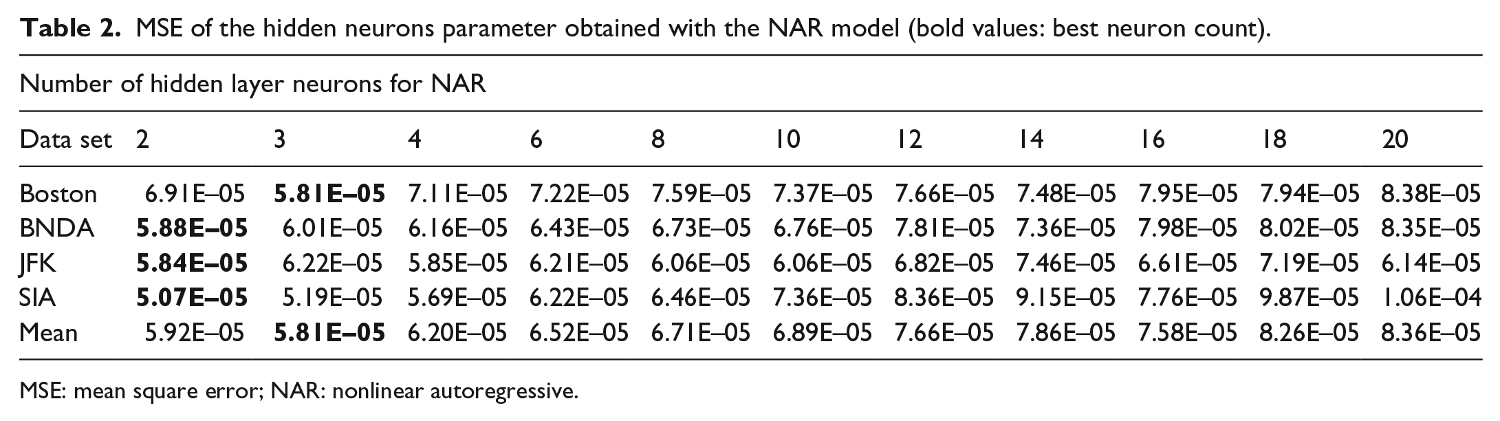
MSE: mean square error; NAR: nonlinear autoregressive.

After this experimentation was completed, the best NAR networks for predicted wind speed for the four different data sets were determined. Figure 8 illustrates the best and the worst trained networks for the 365 days for hourly wind speed data for the Bismarck Municipal Airport (BNDA). Figure 8(a) shows validation performance of 1.2978E–03 and regression values of 0.989. Figure 8(b) shows the validation performance of 5.578E–05 and a regression value of 0.999.

Figure 8.

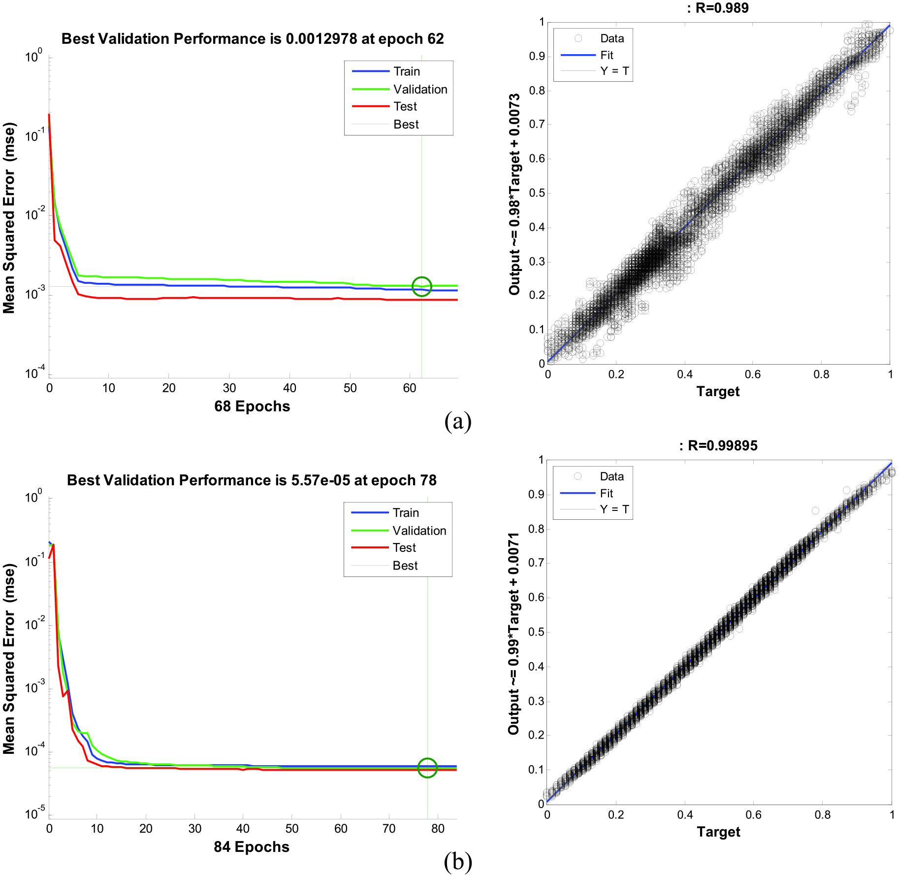
(a) Validation performance and regression values for the worst MSE; (b) validation performance and regression values for the best MSE for the normalized data of BNDA using the NAR model.

The NARX model was tested in a similar fashion with an extra information that could be useful for prediction. In this experiment, dry bulb temperature in Fahrenheit was used as an exogenous input variable. Table 3 illustrates the results pertaining to the number of delays required to obtain the best model. With the NARX network, the best delays were between 28 and 48 h, while the worst delays were generally under 18 h.

Table 3.

MSE of the delay parameter obtained with the NARX model (bold values: best delay).

NARX delays
Data set	2	3	4	6	8	10	12	14	16
Boston	7.66E–04	8.10E–04	7.38E–04	7.81E–04	9.95E–04	9.94E–04	1.11E–03	1.06E–03	1.08E–03
BNDA	1.05E–03	7.64E–04	8.65E–04	1.23E–03	1.32E–03	1.01E–03	8.13E–04	9.42E–04	9.73E–04
JFK	9.80E–04	8.34E–04	8.95E–04	8.92E–04	6.69E–04	7.83E–04	9.13E–04	8.01E–04	9.42E–04
SIA	9.80E–04	8.34E–04	8.95E–04	8.92E–04	6.69E–04	7.83E–04	9.13E–04	8.01E–04	9.42E–04
Mean	9.45E–04	8.10E–04	8.48E–04	9.49E–04	9.13E–04	8.93E–04	9.37E–04	9.01E–04	9.84E–04
Data set	18	20	24	26	28	36	48	60	72
Boston	6.72E–04	6.58E–04	1.54E–04	8.17E–05	7.53E–05	7.99E–05	7.88E–05	7.68E–05	8.13E–05
BNDA	1.11E–03	1.12E–03	1.77E–04	6.68E–05	6.53E–05	6.72E–05	7.58E–05	7.39E–05	7.50E–05
JFK	1.05E–03	8.70E–04	1.37E–04	6.98E–05	6.62E–05	6.78E–05	6.28E–05	6.76E–05	6.76E–05
SIA	1.05E–03	8.70E–04	1.37E–04	6.98E–05	6.62E–05	6.78E–05	6.28E–05	6.76E–05	6.76E–05
Mean	9.73E–04	8.80E–04	1.51E–04	7.20E–05	6.82E–05	7.06E–05	7.01E–05	7.15E–05	7.29E–05

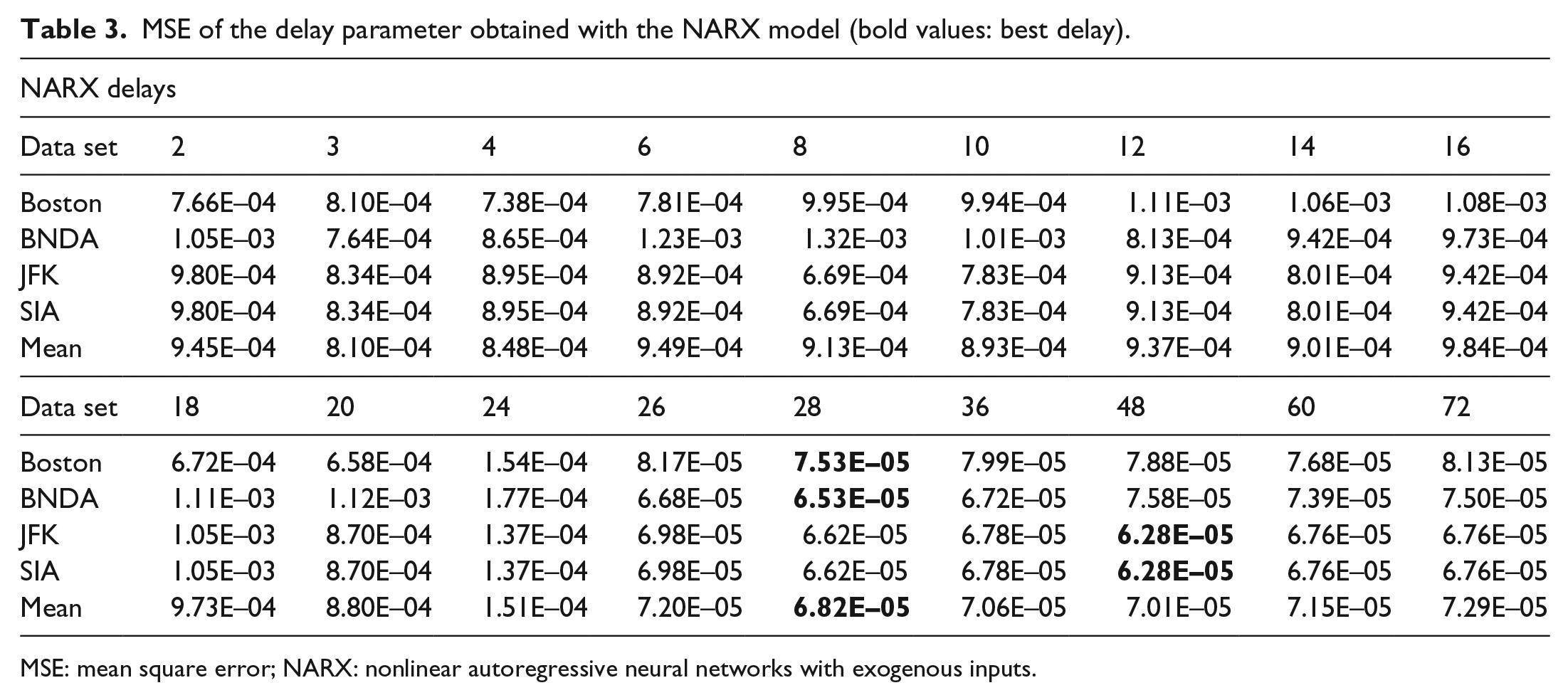
MSE: mean square error; NARX: nonlinear autoregressive neural networks with exogenous inputs.

As was done for the NAR model, Table 4 illustrates the neuron values corresponding to the best MSE for that data set. The best results were achieved between three and six neurons with the average neuron count being three.

Table 4.

MSE of the hidden neurons parameter obtained with the NARX model (bold values: best neuron count in the hidden layer).

Number of hidden layer neurons for NARX
Data set	2	3	4	6	8	10	12	14	16	18	20
Boston	7.06E–05	5.61E–05	7.08E–05	7.07E–05	6.83E–05	7.44E–05	7.26E–05	7.23E–05	7.18E–05	7.23E–05	7.26E–05
BNDA	5.71E–05	5.64E–05	5.84E–05	6.29E–05	6.55E–05	6.47E–05	6.66E–05	6.48E–05	6.77E–05	6.95E–05	6.46E–05
JFK	6.04E–05	6.16E–05	5.96E–05	6.15E–05	6.11E–05	6.26E–05	6.38E–05	6.14E–05	6.33E–05	6.33E–05	6.49E–05
SIA	5.41E–05	5.04E–05	5.06E–05	4.99E–05	5.17E–05	5.57E–05	5.19E–05	5.15E–05	5.49E–05	5.16E–05	5.43E–05
Mean	6.06E–05	5.61E–05	5.98E–05	6.13E–05	6.16E–05	6.44E–05	6.37E–05	6.25E–05	6.44E–05	6.42E–05	6.41E–05

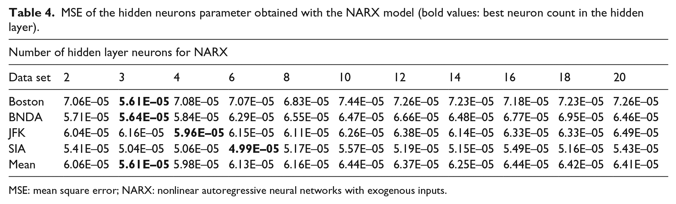
MSE: mean square error; NARX: nonlinear autoregressive neural networks with exogenous inputs.

After this experimentation was completed, the best NARX networks for predicted wind speed for the four different data sets were determined. Figure 9 illustrates the best and the worst trained networks for the 365 days for hourly wind speed data for the Bismarck Municipal Airport (BNDA). Figure 9(a) shows validation performance of 6.5897E–04 and regression values of 0.994. Figure 9(b) shows the validation performance of 5.4767E–05 and a regression value of 0.999.

Figure 9.

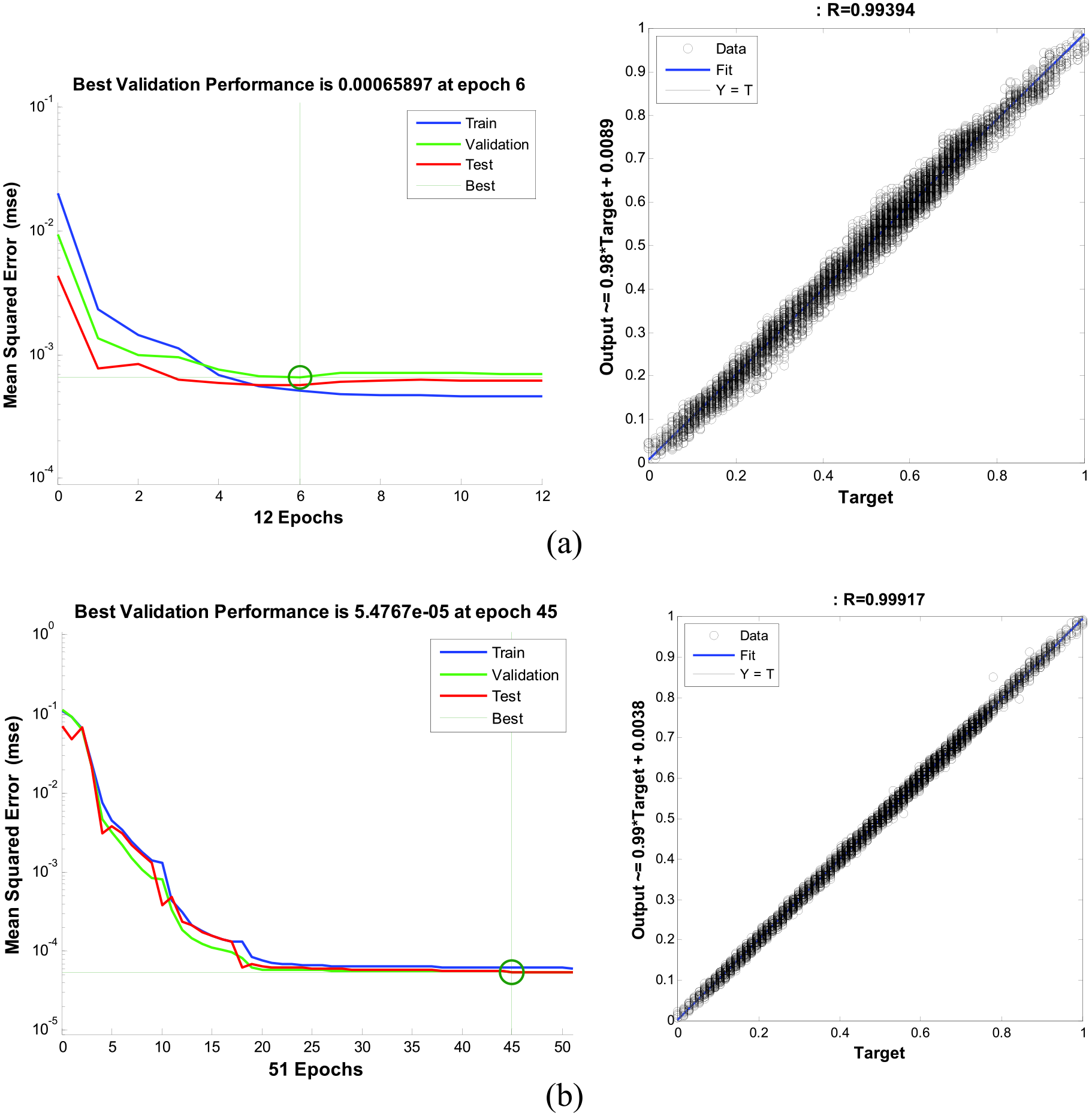
(a) Validation performance and regression values for the worst MSE; (b) Validation performance and regression values for the best MSE for the normalized data of BNDA using the NARX model.

From the presented results, it can be concluded that using an NARX network may reduce the number of previous data points needed to get an accurate prediction; however, neuron counts must be increased yielding a more complex model. A summary of these results is presented in Table 5. Figure 10 shows a comparison between the means obtained from the NAR and NARX models with different number of delays and number of neurons. Both of these plots show that the NARX results have lower error and therefore better performance for predicting wind speed.

Table 5.

Number of neurons and delays corresponding to the lowest MSE values for both NAR and NARX methods.

Number of hidden layer neurons
Data set	NAR	NARX
Boston	3	3
BNDA	2	3
JFK	2	4
SIA	2	6
Mean	2	4
Number of delays
Data set	NAR	NARX
Boston	60	28
BNDA	48	28
JFK	72	48
SIA	60	48
Mean	60	38

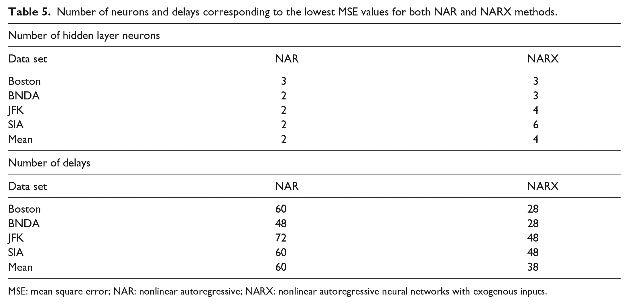
MSE: mean square error; NAR: nonlinear autoregressive; NARX: nonlinear autoregressive neural networks with exogenous inputs.

Figure 10.

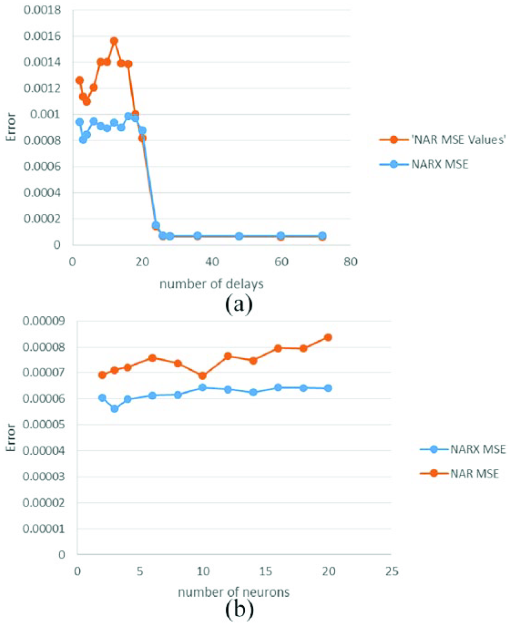
(a) Comparison of average MSE in respect to the delay parameter and (b) comparison of the average MSE in respect to the network complexity (number of hidden layer neurons).

Implementation of optimized networks into step ahead and multi-step-ahead prediction

After the network architecture had been optimized, the NAR and NARX networks were subjected to single-step-ahead and multi-step-ahead prediction. Table 6 shows a comparison between the mean values obtained from 10 trials of the NAR and NARX methods for single-step-ahead and multi-step-ahead predictions. The table displays information illustrating that the NARX results have lower error and therefore better performance for predicting wind speed for single-step-ahead prediction. The multi-step-ahead prediction was much better with the NARX network with two orders of magnitude less error when predicting wind speed 5 h in advance with the addition of the exogenous data. The single-step-ahead results of NAR and NARX models were compared with simple baseline persistence model (Milligan et al., 2003). The results are presented in Table 6. The root mean square error (RMSE) ratio (persistence/NAR and persistence/NARX) are shown in Figure 11. The better performance of NAR and NARX than the baseline persistence model is clearly seen in Table 6 and Figure 11. The MSE error of NAR and NARX models are one to two order of magnitude lower than that obtained from persistence model. The RMSE ratio for NAR varied in the range of 1.97–3.12 and that for NARX varied between 6.12 and 9.89, as shown in Figure 11. This confirmed the better performance of the ANN models than the baseline persistence model. Tables 7 and 8 display the results of paired t-test for both single-step-ahead and multi-step-ahead predictions. The paired t-test confirmed that the difference in results of NAR and NARX models for each case was statistically significant.

Table 6.

Single-step-ahead and multi-step-ahead MSE values for both NAR and NARX methods and all data sets: (a) single-step and (b) multi-step.

Single-step-ahead MSE
Data set	NAR	NARX	Persistence
Boston	7.066E–04	7.306E–05	2.734E–03
BNDA	5.871E–04	5.808E–05	4.824E–03
JFK	5.815E–04	3.440E–05	2.829E–03
SIA	5.853E–04	5.844E–05	5.714E–03
Mean	6.151E–04	5.600E–05	4.025E–03
Multi-step-ahead MSE
Data set	NAR	NARX
Boston	5.599E–03	2.448E–04
BNDA	3.038E–02	9.524E–05
JFK	2.447E–02	6.460E–05
SIA	9.104E–02	7.645E–05
Mean	3.787E–02	1.203E–04

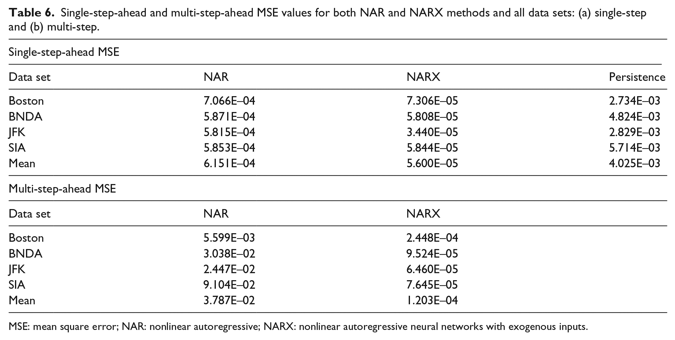
MSE: mean square error; NAR: nonlinear autoregressive; NARX: nonlinear autoregressive neural networks with exogenous inputs.

Figure 11.

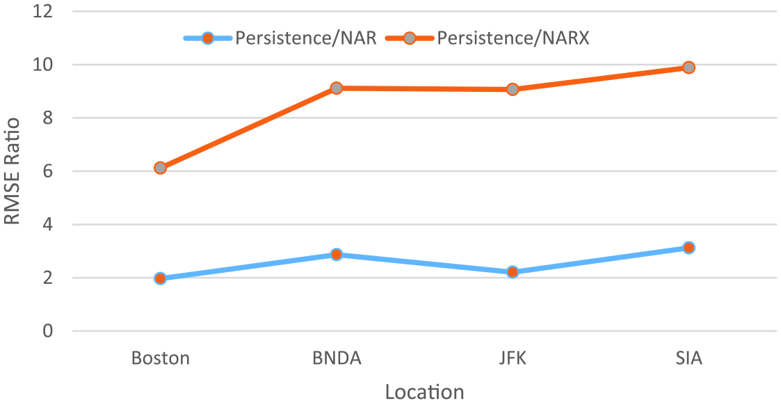
Comparison of RMSE ratio for NAR and NARX models over persistence model.

Table 7.

Summary of paired t-test results for single-step-ahead prediction of wind speed.

Data set	Method	df	Mean	Standard deviation	SE mean	95% CI for mean difference	t-statistic (H0: diff = 0, H1: diff not 0)	p-value
Boston	NAR	10	0.000707	0.000016	0.000005	0.000621, 0.000646	115.67	0.000
	NARX	10	0.000073	0.000002	0.000001
	Difference	10	0.000634	0.000017	0.000005
BNDA	NAR	10	0.000587	0.000023	0.000007	0.000513, 0.000545	72.65	0.000
	NARX	10	0.000058	0.000001	0.000000
	Difference	10	0.000529	0.000023	0.000007
JFK	NAR	10	0.000581	0.000036	0.000011	0.000521, 0.000573	47.63	0.000
	NARX	10	0.000034	0.000006	0.000002
	Difference	10	0.000547	0.000036	0.000011
SIA	NAR	10	0.000585	0.000021	0.000007	0.000511, 0.000542	77.18	0.000
	NARX	10	0.000058	0.000002	0.000001
	Difference	10	0.000527	0.000022	0.000007

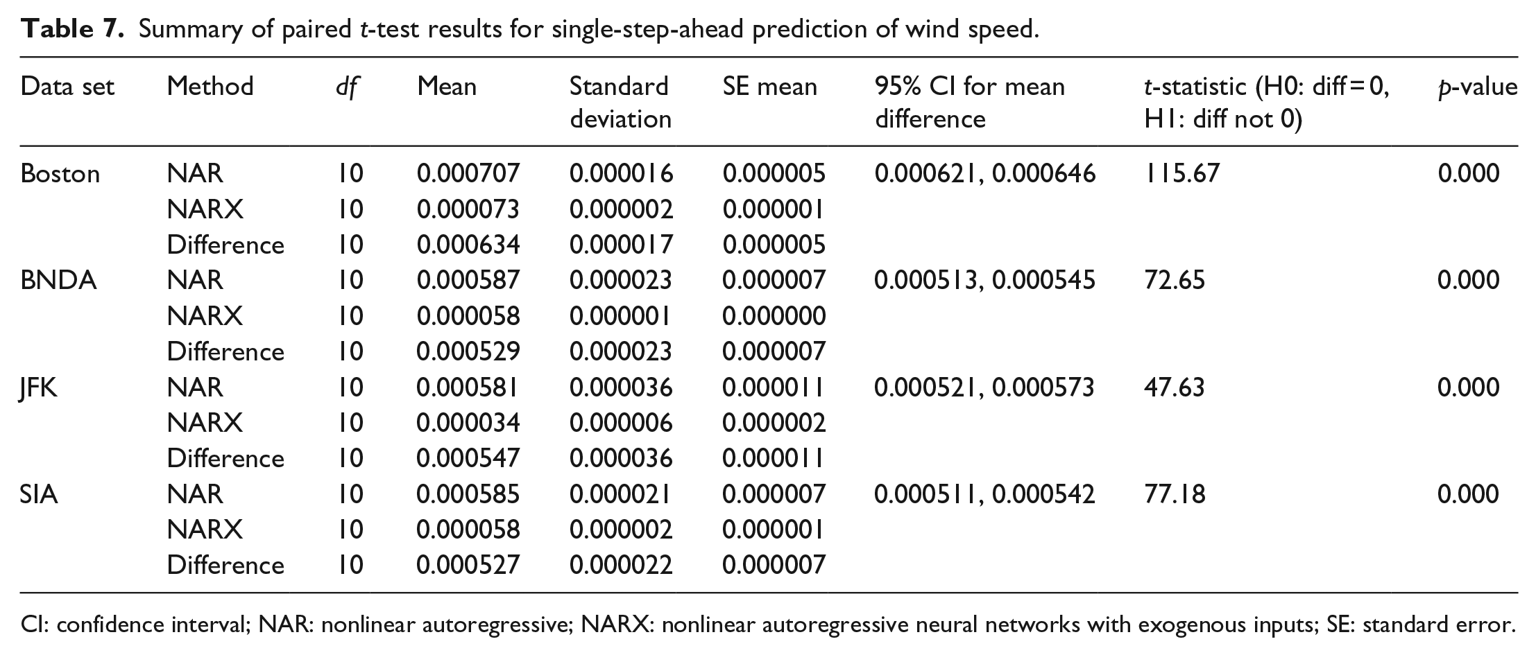
CI: confidence interval; NAR: nonlinear autoregressive; NARX: nonlinear autoregressive neural networks with exogenous inputs; SE: standard error.

Table 8.

Summary of paired t-test results for multi-step-ahead prediction of wind speed.

Data set	Method	df	Mean	Standard deviation	SE mean	95% CI for mean difference	t-statistic (H0: diff = 0, H1: diff not 0)	p-value
Boston	NAR	10	0.005599	0.000271	0.000086	0.005082, 0.005626	44.53	0.000
	NARX	10	0.000245	0.000165	0.000052
	Difference	10	0.005354	0.000380	0.000120
BNDA	NAR	10	0.030380	0.002518	0.000796	0.028481, 0.032089	37.97	0.000
	NARX	10	0.000095	0.000013	0.000004
	Difference	10	0.030285	0.002522	0.000798
JFK	NAR	10	0.024470	0.001819	0.000575	0.023101, 0.025709	77.18	0.000
	NARX	10	0.000065	0.000007	0.000002
	Difference	10	0.024405	0.001823	0.000577
SIA	NAR	10	0.09104	0.00389	0.00123	0.08818, 0.09374	73.91	0.000
	NARX	10	0.00008	0.00000	0.00000
	Difference	10	0.09096	0.00389	0.00123

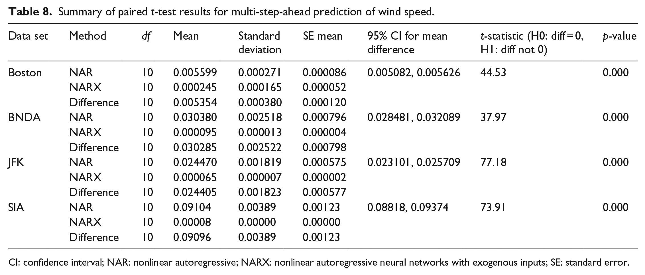
CI: confidence interval; NAR: nonlinear autoregressive; NARX: nonlinear autoregressive neural networks with exogenous inputs; SE: standard error.

Figures of the normalized target values and the corresponding predicted values using NAR and NARX networks for each data set were plotted to examine visually the effectiveness of the models. Figures for one the locations (JFK) are presented in Figures 12 and 13 for NAR and NARX models for single-step (1-h)-ahead and multi-step (5-h)-ahead wind speed prediction. Figure 12 presents NAR and NARX results for JFK data set for 1-h-ahead prediction, and Figure 13 shows 5-h-ahead prediction. While hourly predictions were made, these plots are displayed in time steps of 48 h for better legibility. For single-step-ahead prediction both NAR and NARX models predicted the wind speed quite reasonably well, though NARX predictions were closer to the actual data. For 5-h-ahead predictions, NARX outperformed NAR by a wide a margin as the NARX predictions were mostly much closer to the actual data compared to the NAR predicted data. Other results showed similar trends with better prediction from NARX than NAR. The differences in prediction performance of NARX and NAR models were much more prominent for multi-step-ahead prediction than single-step-ahead prediction as presented in Table 6.

Figure 12.

Single-step-ahead comparison of target values versus predicted in the JFK Airport data set: (a) NAR network and (b) NARX network (48 h time steps).

Figure 13.

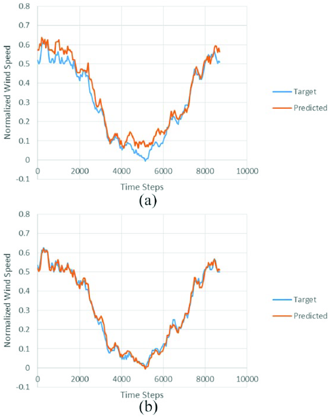
Multi-step-ahead prediction comparison of target values versus predicted in the JFK Airport data set: (a) NAR network and (b) NARX network (48 h time steps).

Discussion

This experimentation has concentrated on the comparison of prediction performances of NAR and NARX network models for wind speed forecasting, and these networks consider cases where exogenous data are available or not. The first issue to be confronted when selecting the model to be used is the availability of data when trying to perform prediction. Most wind generation efforts will include a meteorological tower that will collect wind speed data as well other categories of data useful for wind speed prediction.

In the network architecture optimization section of the study, it is important to note the importance of the number of delays chosen when optimizing this type of model. Table 5 shows that each data set had a different optimized delay parameter and its value cannot be generalized for all data sets. The delay parameter is important as each data set has its own characteristics and behavior as seen in Figure 7. It was found that the use of external data such as temperature can lower the amount of delays needed to get accurate predictions in every case observed. NARX requires fewer past values and thus NARX prediction models will be simpler.

NAR methods were determined to be useful if only wind speed information was available and can provide accurate midterm predictions. This simpler alternative to the NARX method can be used with a simple data set only containing wind speed data. Table 1 shows that an NAR model with little information, such as only 2 h of delay, is not an adequate amount of information to model the data and provides poor results when compared to higher number of delays. The highest accuracy for the NAR model was averaged at 60 h of previous data. A higher number of delays more than 28 may be not necessary as the accuracy is basically stabilized at this point as seen in Figure 10(a).

It was determined that a less complex model regarding the number of neurons in the hidden layer yielded a time series that modeled the target time series well. A higher number of neurons in the hidden layer deteriorated prediction results due to the local optima in the network parameters’ optimization process during the training stage. Suitable predictions were obtained as seen in Figure 10(b). The number of hidden layer neurons varied between 2 and 3 (NAR) to 3 and 6 (NARX).

NARX methods have illustrated that the inclusion of another simple time series, such as dry bulb temperature, can help explain anomalies and sudden changes in wind speed and, thus, create a more accurate time series forecast. For example, it can be seen in Figure 1 that temperature and wind speed have a somewhat inverse relationship. If the temperature were to fluctuate suddenly preemptively to a wind speed change, the model would be able to take this into account and thus would give a more accurate prediction.

Due to this extra time series, the NARX methods tend to need less data in order to get a reasonable prediction. As seen in Table 5, each data set required a different delay parameter in order to get optimal results. The average delay for best results was 28 h of previous data, and this is where the data stabilized as seen in Figure 10(a). It can also be observed from this figure that when less than 28 h of data are given in the delays, the NARX network performs much better.

The number of neurons present in the NARX network was on average best at three with the Savannah International Airport data set having the lowest MSE values with six neurons. Network complexity is about the same for both NARX and NAR networks. NARX networks required less historical data to get a more accurate prediction as displayed in Figure 10(b). This shows that the model was able to adjust itself very well to the curve of real data, a better fit than the NAR data.

To summarize the optimization portion of the study, Figure 10(a) and (b) provides a clear graphical representation of the models. NAR methods are good if only wind speed data are available. NAR methods work with a simpler data set; however, more of the historic data are needed to have a good forecast. Conversely, NARX models work with exogenous data, and this allows the model to have simpler predictors by imputing additional data. Figure 10(b) illustrates the final results of neuron optimization in the NAR and NARX networks. This figure shows that the NARX network improves upon the NAR network, actually the worst result obtained by the NARX network is still better than the best NAR results in most cases.

When the optimized networks were implemented in single-step- and multi-step-ahead prediction models the differences continued to grow. When observing the single-step-ahead MSE values (Table 6), it can be seen that the NAR network had values averaging at 6.1994E–04, while the NARX networks had values averaging at 5.561E–05, a difference in an order of magnitude. The NARX network was able to outperform the NAR network in single-step predictions. When observing the multi-step-ahead predictions from the same table, NAR averaged 3.850E–02, while NARX averaged at 1.043E–04, a difference of two orders of magnitude. However, both these models were far superior to the baseline persistence model as shown in Table 6 and Figure 11.

The NARX network significantly outperformed the NAR network when predicting five time steps in advance. This furthers the conclusion that NARX networks require less data in order to get a more accurate prediction that is able to adjust itself very well to the curve of real data, a much better fit than the NAR network. This comparison can be noted graphically in Figures 12 and 13. The NARX networks are seen to outperform the NAR networks in single-step-ahead prediction in all locations. This effect is compounded when observing the multi-step-ahead prediction for all four locations. The NARX network greatly outperformed the NAR network in a 5-h-ahead prediction. The difference in prediction performance of NARX and NAR models was statistically significant.

Conclusion

The study presented a methodology to forecast wind speed using artificial neural networks. This method used 1 year’s worth of hourly wind data in mile/h and dry bulb temperature data in degrees Fahrenheit from four different locations in the United States. The data were normalized in the range between 0 and 1 in order to compare results between different data sets and prevent local extrema from skewing results. Two ANN prediction models, NAR and NARX, were used. Both time series prediction models gave acceptable results; however, it was found that performance of NARX, with an addition of external data of dry bulb temperature, was better than NAR model. NARX also had the advantage of using less delays, meaning less historical data were used in forecasting. When forecasting 1 h ahead, the NARX network had error one order of magnitude less than the NAR network. When forecasting 5 h ahead, the NARX network had error two orders of magnitude less than the NAR network. This furthers the conclusion that NARX networks require less data in order to get a more accurate prediction than the NAR network. Both these ANN-based models outperformed the baseline persistence model.

The wind speed prediction could potentially be improved by employing other ANN techniques, with additional weather data. Incorporating numerical weather prediction algorithms could potentially increase the time frame these models are able to predict accurately as well. It would be interesting to include more exogenous data into the model in order to determine if this would increase the accuracy of the current model. These would be subjects of further research.

Footnotes

Declaration of conflicting interests

The author(s) declared no potential conflicts of interest with respect to the research, authorship, and/or publication of this article.

Funding

The author(s) received no financial support for the research, authorship, and/or publication of this article.

References

Berge

(2002) Experiences with wind forecasting techniques in Norway. In: Proceedings of the first joint action symposium on wind forecasting technique, Norrköping, pp. 59–64. Paris: International Energy Agency (IEA), December 2002.

Brand

Kok

(2002) Wind power by a quarter of the hour. In: Proceedings of the first joint action symposium on wind forecasting techniques, Norrköping, pp. 163–169. Paris: International Energy Agency (IEA), December 2002.

Camara

Feixing

Xiuqin

(2016) Energy consumption forecasting using seasonal ARIMA with artificial neural networks models. International Journal of Business & Management 11(5): 231–243.

Cao

Ewing

Thompson

(2012) Forecasting wind speed with recurrent neural networks. European Journal of Operational Research 221: 148–154.

Cigizoglu

Kisi

(2005) Flow prediction by three back propagation techniques using k-fold partitioning of neural network training data. Nordic Hydrology 36(1): 1–16.

Doucoure

Agbossou

Cardenas

(2016) Time series prediction using artificial wavelet neural network and multi-resolution analysis: Application to wind speed data. Renewable Energy 92: 202–211.

Fadare

(2010) The application of artificial neural networks to mapping of wind speed profile for energy application in Nigeria. Applied Energy 87: 934–942.

Hagan

Demuth

Beale

(1996) Neural Network Design. Boston, MA: PWS Pub. Co.

Haydari

Kavehnia

Askari

(2007) Time-series load modelling and load forecasting using neuro-fuzzy techniques. In: Proceedings of the 9th international conference on electrical power quality and utilization, Barcelona, 9–11 October.

10.

Jursa

(2007) Wind power prediction with different artificial intelligence models. In: Proceedings of the European wind energy conference (EWEC), Milan, 2007. Available at: http://citeseerx.ist.psu.edu/viewdoc/summary?doi=10.1.1.174.8568

11.

Kaminsky

Kirchhoff

Sheu

(1985) Time series models of average wind speed within synoptic weather categories. In: Proceedings of the fourth ASME wind energy symposium, pp. 215–219. New York: American Society of Mechanical Engineers. Dallas, TX, 17–21 February, 1985.

12.

Kariniotakis

Stavrakakis

Nogaret

(1996) Wind power forecasting using advanced neural network models. IEEE Transactions on Energy Conversion 11(4): 762–767.

13.

Kiartzis

Bakirtzis

Petridis

(1995) Short-term forecasting using NNs. Electric Power Systems Research 33: 1–6.

14.

Lei

Shiyan

Chuanwen

(2009) A review on the forecasting of wind speed and generated power. Renewable & Sustainable Energy Reviews 13(4): 915–920.

15.

Macas

Moretti

Fonti

(2016) The role of data sample size and dimensionality in neural network based forecasting of building heating related variables. Energy and Buildings 111: 299–310.

16.

Marquardt

(1963) An algorithm for least-squares estimation of nonlinear parameters. Journal of the Society for Industrial and Applied Mathematics 11: 431–441.

17.

Mathworks (2017) Neural Network Toolbox: User’s Guide (R2017a). Natick, MA: The MathWorks Inc.

18.

Milligan

Schwartz

Wan

(2003) Statistical wind power forecasting models: Results for U.S. wind farms. In: WINDPOWER 2003, Austin, TX, 18–21 May, NREL/CP-500-33956. Available at: https://www.nrel.gov/docs/fy03osti/33956.pdf

19.

Mohanty

Patra

Sahoo

(2015) Prediction of global solar radiation using nonlinear auto regressive network with exogenous inputs (NARX). In: Proceedings of 39th national systems conference (NSC), Noida, India, 14–16 December.

20.

Deo

(2003) Forecasting wind with neural networks. Marine Structures 16(1): 35–49.

21.

Nagy

(2016) Probabilistic solar and wind power forecasting using a generalized additive tree ensemble approach. International Journal of Forecasting 32(3): 1087–1093.

22.

National Oceanic and Atmospheric Administration (NOAA) National Centers for Environmental Information (2010) Climate data online, normal hourly averages. Available at: https://www.ncdc.noaa.gov/cdo-web/

23.

Samanta

(2004) Gear fault detection using artificial neural networks and support vector machines with genetic algorithms. Mechanical Systems and Signal Processing 18(3): 625–644.

24.

Samanta

(2011) Prediction of chaotic time series using computational intelligence. Expert Systems with Applications 38(9): 11406–11411.

25.

Sanchez

(2008) Adaptive combination of forecasts with application to wind energy. International Journal of Forecasting 24(4): 679–693.

26.

Sfetsos

(2000) A comparison of various forecasting techniques applied to mean hourly wind speed time series. Renewable Energy 21(1): 21–35.

27.

Tande

Landberg

(1993) A 10 sec forecast of wind turbine output with neural networks. In: Proceedings of European community wind energy conference, Travemünde, 8–12 March, pp. 774–777. Bedford: H.S. Stephens and Associates.

28.

Torres

Garcia

Deblas

(2005) Forecast of hourly average wind speed with ARIMA models in Navarre (Spain). Solar Energy 79(1): 65–77.

29.

US Department of Energy (2015) Wind vision: A new era for wind power in the United States. Available at: https://www.energy.gov/sites/prod/files/WindVision_Report_final.pdf

30.

Welch

Ruffing

Venayagamoorthy

(2009) Comparison of feedforward and feedback neural network architectures for short-term wind speed prediction. In: Proceedings of international joint conference on neural networks, Atlanta, GA, 14–19 June.

31.

Benoit

Girard

(2006) Wind energy simulation toolkit (WEST): A wind mapping system for use by the wind-energy industry. Wind Engineering 30(1): 15–33.