Small signal stability analysis of power systems integrated with wind power using sensitivity-based index

Abstract

To know the inherent property of the power system connected with a wind farm along with its associated controllers, a small signal stability study is required. For this, a linearized system model has to be developed. The small signal model of the system with wind farm along with its controllers is discussed here. The eigenvalues of system matrix are computed from the linearized model of the power system. The absolute value of the real part of eigenvalues indicates distance from instability. The sensitivity of this minimum real part of eigenvalues with respect to small changes of wind power injection is used as an index to assess the small signal stability under various operating conditions. The optimum value of the wind power can also be determined with the help of the proposed eigenvalue sensitivity index. The systems used for the study are WSCC 3-machine 9-bus system and IEEE 16-machine 68-bus system.

Keywords

Eigenvalue sensitivity index small signal stability wind power multi-machine system

Introduction

The depleting fossil fuels and their environmental impact raise the penetration of more and more renewable sources into the grid. This brings concern about the stability of the existing power system, as these sources are intermittent and variable in nature. Wind energy, being cheapest till date, is used extensively all across the globe. As the share of wind power increases, its impact on the power system stability becomes a major concern. A study of the inherent stability of large power systems with wind farms and its associated controllers (e.g. the doubly fed induction generator (DFIG) converter controllers, pitch controller) is also quite important. This requires a small signal stability analysis using linearized system equations. Small signal stability study of power system with increased wind power penetration is presented in Gautam et al. (2009), Bu et al. (2012) and Wang et al. (2008). A simplified model of DFIG is proposed for the small signal stability study of the power system in Wang et al. (2008). Modal analysis of the DFIG-based wind power generation system, to observe the change in modal properties for different system parameters, operating points and grid strengths, is presented in Mei and Pal (2007). Small signal stability study of power systems with variable wind power is presented in Garmroodi et al. (2014). The sensitivity indices based on the eigenvalues are used for the power system small signal stability studies as in Gautam et al. (2009), Nam et al. (2000), Nolan et al. (1976) and Wang et al. (2000). However, a detailed study including the dynamics of both the power system and the wind farm along with its controllers may be of help.

In this article, a detailed modelling of DFIG-based wind farm along with its converters is presented to study the small signal stability analysis in different cases, such as (a) wind speed below rated value and (b) wind speed above rated value. The dominant states (the state variables of the power system integrated with DFIG-based wind farms), that is, the states which are affected most, are also found out to understand the internal small signal dynamics of the system considered. A new sensitivity-based index is proposed to see the impact of wind power penetration on the system small signal stability and thereby identify the optimum limit of wind power injection to the existing system without affecting the overall stability (small signal) of the system.

Small signal model of multi-machine power system

Small signal model for the system without wind farm

The flux decay model of multi-machine power system (Kundur, 1994), with m machines, is considered. The linearized model of the system can be written in a compact form as

Δ \overset{\cdot}{X} = A_{1} Δ X + A_{2} Δ I_{g} + A_{3} Δ V_{g} + E_{1} Δ U

(1)

0 = B_{1} Δ X + B_{2} Δ I_{g} + B_{3} Δ V_{g}

(2)

0 = C_{1} Δ X + C_{2} Δ I_{g} + C_{3} Δ V_{g} + C_{4} Δ V_{l}

(3)

0 = D_{1} Δ V_{g} + D_{2} Δ V_{l}

(4)

where,

\begin{array}{l} Δ X = {[\begin{matrix} Δ δ_{1} \dots Δ δ_{m} & Δ ω_{1} \dots Δ ω_{m} & Δ {E^{'}}_{q_{1}} \dots Δ {E^{'}}_{q_{m}} & Δ E_{f d_{1}} \dots Δ E_{f d_{m}} \end{matrix}]}^{T} \\ Δ I_{g} = {[\begin{matrix} Δ I_{d 1} & Δ I_{q 1} \dots Δ I_{d m} & Δ I_{q m} \end{matrix}]}^{T} \\ Δ V_{g} = {[\begin{matrix} Δ θ_{1} & Δ V_{1} \dots Δ θ_{m} & Δ V_{m} \end{matrix}]}^{T} \\ Δ V_{l} = {[\begin{matrix} Δ θ_{m + 1} & Δ V_{m + 1} \dots Δ θ_{n} & Δ V_{n} \end{matrix}]}^{T} \\ Δ u = {[\begin{matrix} Δ P_{m_{1}} & Δ V_{r e f_{1}} \dots Δ P_{m_{m}} & Δ V_{r e f_{m}} \end{matrix}]}^{T} \end{array}

Here, δ is the angular position of the rotor, ω_i is per unit speed deviation of the rotor, P_m is mechanical power input, ${E'}_{d}$ and $E_{'}^{q}$ are the d-axis and q-axis components of voltages behind the transient reactance, $I_{d}$ and $I_{q}$ are the d-axis and q-axis currents, V is the terminal voltage of the machine in per unit and θ is its angle, equations (1) to (4) together represent the linearized model for multi-machine power system. A₁, A₂, A₃, B₁, B₂, B₃, C₁, C₂, C₃, C₄, D₁, D₂ and E₁ are the coefficient matrices in the linearized model. Equations (1) to (4) can be put together and written as

[\begin{array}{l} Δ \overset{\cdot}{X} \\ 0 \\ 0 \\ 0 \end{array}] = [\begin{array}{l} A_{1} & A_{2} & A_{3} & 0 \\ B_{1} & B_{2} & B_{3} & 0 \\ C_{1} & C_{2} & C_{3} & C_{4} \\ 0 & 0 & D_{1} & D_{2} \end{array}] [\begin{array}{l} Δ X \\ Δ I_{g} \\ Δ V_{g} \\ Δ V_{l} \end{array}] + [E_{1}] [Δ u]

(5)

This can be reduced to the form

Δ \overset{\cdot}{X} = A_{s y s} Δ X + E_{1} Δ u

(6)

where the system matrix A_sys of the power system is given by

A_{s y s} = [A_{1}] - [\begin{array}{l} A_{2} & A_{3} & 0 \end{array}] {[\begin{array}{l} B_{2} & B_{3} & 0 \\ C_{2} & C_{3} & C_{4} \\ 0 & D_{1} & D_{2} \end{array}]}^{- 1} [\begin{array}{l} B_{1} \\ C_{1} \\ 0 \end{array}]

(7)

Small signal model for the power system with wind farm

Linearized model of DFIG

The DFIG-based wind farm is connected to one load bus of the power system (Figure 1). An aggregated wind turbine and aggregated DFIG are considered for representing the wind farm. The wind farm is connected to one of the existing power system buses (bus ‘m’ in Figure 1) through a transformer and a double circuit line. The terminal bus of the wind farm (bus ‘n’ in Figure 1) is included in the power system as an additional bus. If multiple wind farms are present (say n_dg number), then there will be n_dg number of additional buses in the power system.

Figure 1.

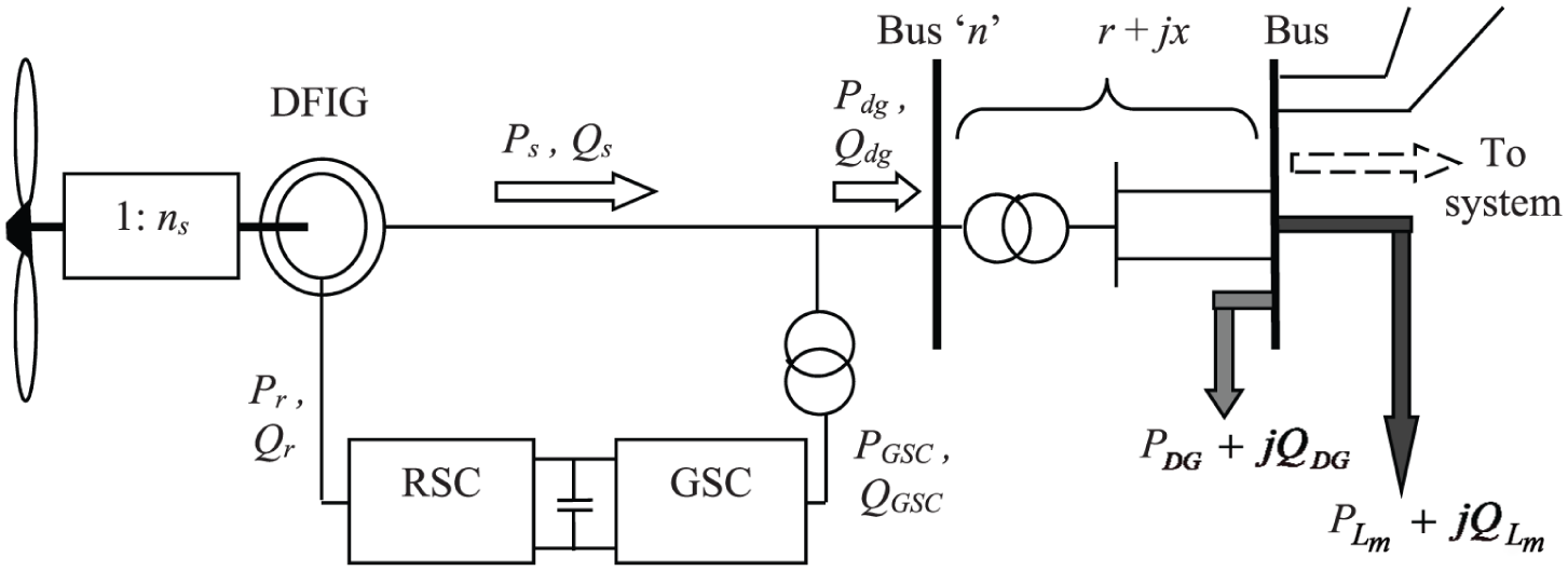
Connection of DFIG to the system load bus.

The set of differential algebraic equations (DAEs) of the DFIG (Mitra and Chatterjee, 2016) can be linearized to obtain

\frac{d Δ i_{d s i}}{d t} = \frac{ω_{b a s e}}{{L^{'}}_{s i}} [- (R_{s i} + \frac{(L_{s s i} - {L^{'}}_{s i})}{T_{r i}}) Δ i_{d s i} - {L^{'}}_{s i} Δ i_{q s i} + \frac{Δ {e^{'}}_{q i}}{T_{r i}} + ω_{r i} Δ {e^{'}}_{d i} + {e^{'}}_{d i} Δ ω_{r i} + K_{m r r i} Δ v_{d r i} - Δ v_{d s i}]

(8)

\frac{d Δ i_{q s i}}{d t} = \frac{ω_{b a s e}}{{L^{'}}_{s i}} [- (R_{s i} + \frac{(L_{s s i} - {L^{'}}_{s i})}{T_{r i}}) Δ i_{q s i} - {L^{'}}_{s i} Δ i_{d s i} + \frac{Δ {e^{'}}_{d i}}{T_{r i}} + ω_{r i} Δ {e^{'}}_{q i} + {e^{'}}_{q i} Δ ω_{r i} + K_{m r r i} Δ v_{q r i} - Δ v_{q s i}]

(9)

\frac{d Δ {e^{'}}_{d i}}{d t} = ω_{b a s e} [ω_{s} \frac{(L_{s s i} - {L^{'}}_{s i})}{T_{r i}} Δ i_{q s i} - \frac{Δ {e^{'}}_{d i}}{T_{r i}} + ω_{s} (ω_{s} - ω_{r i}) Δ {e^{'}}_{q i} - ω_{s} {e^{'}}_{q i} Δ ω_{r i} - ω_{s} K_{m r r i} Δ v_{q r i}]

(10)

\frac{d Δ {e^{'}}_{q i}}{d t} = ω_{b a s e} [- ω_{s} \frac{(L_{s s i} - {L^{'}}_{s i})}{T_{r i}} Δ i_{d s i} - \frac{Δ {e^{'}}_{q i}}{T_{r i}} - ω_{s} (ω_{s} - ω_{r i}) Δ {e^{'}}_{d i} + ω_{s} {e^{'}}_{d i} Δ ω_{r i} + ω_{s} K_{m r r i} Δ v_{d r i}]

(11)

\frac{d Δ ω_{r i}}{d t} = \frac{1}{2 H_{g i}} [k_{s h i} Δ θ_{t w i} + C_{s h i} ω_{b a s e} (Δ ω_{t i} - Δ ω_{r i}) - Δ T_{e i}]

(12)

\frac{d Δ θ_{t w i}}{d t} = ω_{b a s e} (Δ ω_{t i} - Δ ω_{r i})

(13)

\frac{d Δ ω_{t i}}{d t} = \frac{1}{2 H_{t i}} [Δ T_{m i} - k_{s h i} Δ θ_{t w i} - C_{s h i} ω_{b a s e} (Δ ω_{t i} - Δ ω_{r i})]

(14)

Δ P_{d g i} = v_{d s i} Δ i_{d s i} + i_{d s i} Δ v_{d s i} + v_{q s i} Δ i_{q s i} + i_{q s i} Δ v_{q s i} + v_{d r i} Δ i_{d r i} + i_{d r i} Δ v_{d r i} + v_{q r i} Δ i_{q r i} + i_{q r i} Δ v_{q r i}

(15)

Δ Q_{d g i} = v_{q s i} Δ i_{d s i} + i_{d s i} Δ v_{q s i} - v_{d s i} Δ i_{q s i} - i_{q s i} Δ v_{d s i}

(16)

where i = n + 1, . . . n +n_dg; ω_base is the electrical base speed; ω_s is the synchronous speed in per unit; v_ds and v_qs are the stator d-axis and q-axis voltages, respectively; v_dr and v_qr are the rotor d-axis and q-axis voltages, respectively; i_ds and i_qs are the stator d-axis and q-axis currents, respectively; L_ss is stator inductance and R_s is the stator resistance. T_r (=L_rr/R_r) is the rotor time constant where L_rr is rotor inductance and R_r is the rotor resistance. ${e^{'}}_{d}$ and ${e^{'}}_{q}$ are the equivalent d-axis and q-axis source voltage behind transient impedance. ω_r and ω_t are the rotor electrical and mechanical speeds, respectively; θ_tw is the shaft torsional angle; H_t and H_g are the turbine and the generator inertia, respectively and k_sh and C_sh are the shaft stiffness and damping coefficient, respectively.

The complete expressions of ΔP_dgi and ΔQ_dgi in terms of the DFIG state variables and algebraic variables can be obtained from equations (15) and (16). ΔT_mi in equation (14) can be expressed in terms of the DFIG state variables (turbine speed ω_ti and pitch angle β_i) and wind speed (V_w).

DFIG controllers

The rotor circuit of the DFIG is connected to the stator terminal through back to back voltage source converters (Figure 1). These are the rotor side converter (RSC) and the grid side converter (GSC) connected with each other by the DC bus capacitor. Pitch controller is present for the purpose of controlling the DFIG rotor speed when wind speed exceeds the rated value.

RSC controller

The purpose of this controller is to control the DFIG rotor speed by controlling the electrical torque for maximum power extraction from wind. The RSC controller also controls the reactive power exchanged at the stator terminal of DFIG. Field-oriented control (FOC) (Mitra and Chatterjee, 2016; Nunes et al., 2004) technique is used, where the d-axis of the synchronously rotating reference frame is considered to be oriented along the stator (or bus ‘n’ in Figure 1) voltage V_n. The q-axis is considered to be leading the d-axis. Hence, the voltages along the d axis and q axis (v_ds and v_qs, respectively) are given by

v_{d s} = V_{n} and v_{q s} = 0

(17)

For a sufficiently low stator resistance R_s

ψ_{d s} ≅ 0 and ψ_{q s} ≅ ψ_{s}

(18)

Putting the values of i_ds and i_qs in terms of the stator fluxes, we get

T_{e} = L_{m} [\frac{1}{L_{s s}} (ψ_{d s} - L_{m} i_{d r}) i_{q r} - \frac{1}{L_{s s}} (ψ_{q s} - L_{m} i_{q r}) i_{d r}]

(19)

Using equation (19), T_e can be expressed applying equation (18) as a function of d-axis rotor current (i_dr) as

T_{e} = - (\frac{L_{m}}{L_{s s}}) ψ_{q s} i_{d r}

(20)

Putting the value of i_qs in terms of ψ_qs, we get

Q_{s} = v_{q s} i_{d s} - v_{d s} \frac{1}{L_{s s}} (ψ_{q s} - L_{m} i_{q r})

(21)

From equation (21), Q_s can be expressed applying equation (17) as a function of q-axis rotor current (i_qr) as

Q_{s} = (\frac{L_{m} v_{d s}}{L_{s s}}) i_{q r} - v_{d s} \frac{ψ_{q s}}{L_{s s}}

(22)

The rotor voltage equations can be re-written, with the assumption of constant stator flux, in terms of the rotor variables as

v_{d r} = - R_{r} i_{d r} - σ L_{r r} \frac{d}{d t} i_{d r} + (ω_{s} - ω_{r}) (σ L_{r r} i_{q r} + \frac{L_{m}}{L_{s s}} ψ_{q s})

(23)

v_{q r} = - R_{r} i_{q r} - σ L_{r r} \frac{d}{d t} i_{q r} - (ω_{s} - ω_{r}) σ L_{r r} i_{d r}

(24)

Here, σ is the leakage factor given by $σ = 1 - (L_{m}^{2} / L_{s s} L_{r r})$ .

Using equations (20) and (22) to (24), the control structure of the RSC controllers is given as shown in Figure 2 (Mitra and Chatterjee, 2016).

Figure 2.

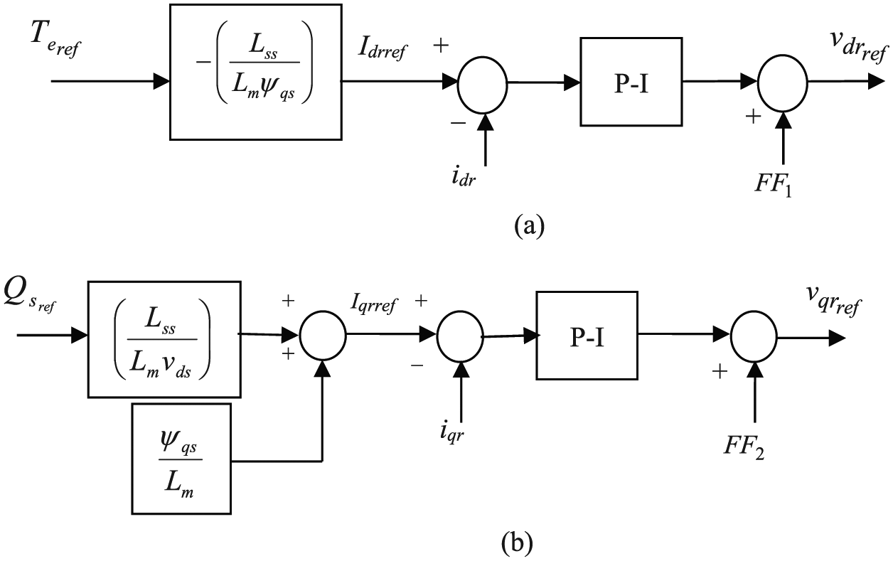
(a) d-axis control block of DFIG rotor side converter and (b) q-axis control block of DFIG rotor side converter.

With $T_{e} = T_{e_{r e f}}$ and $Q_{s} = Q_{s_{r e f}}$ , the expressions for the I_drref and I_qrref can be obtained using equations (20) and (22), respectively. The expressions of the cross-coupling terms FF₁ and FF₂ are as below

F F_{1} = (ω_{s} - ω_{r}) (σ L_{r r} i_{q r} + \frac{L_{m}}{L_{s s}} ψ_{q s})

(25)

F F_{2} = - (ω_{s} - ω_{r}) σ L_{r r} i_{d r}

(26)

In order to extract maximum power from the wind, the torque reference ( $T_{e_{r e f}}$ ) is obtained using the relation (Mitra and Chatterjee, 2016)

T_{e_{r e f}} = K_{o p t} ω_{r}^{2}

(27)

where K_opt in pu is given by

K_{o p t} = \frac{0.5 ρ π R^{5} C_{p_{\max}} ω_{t B}^{2}}{(λ_{o p t}^{3} S_{B})}

(28)

where S_B and ω_tB are the base power and the base speed of the wind turbine, respectively. $C_{p_{\max}}$ is the maximum value of the coefficient of performance of the wind turbine C_p when the pitch angle (β) is 0°; λ_opt is the tip speed ratio when $C_{p} = C_{p_{\max}}$ (Bianchi et al., 2007; Mitra and Chatterjee, 2016).

However, the relation of equation (27) is valid for the speed range $ω_{r} < ω_{r_{r a t e d}}$ .

If the speed ω_{r} \geq ω_{r_{r a t e d}}, T_{e_{r e f}} = T_{e_{r a t e d}}

(29)

Here, $T_{e_{r a t e d}}$ is the rated torque and $ω_{r_{r a t e d}}$ is the rated DFIG speed.

For including the controllers in the small signal stability study, the relationships established in the controllers are expressed in terms of differential and algebraic equations. The equations corresponding to the d-axis control structure are

\frac{d φ_{i d}}{d t} = I_{d r r e f} - i_{d r}

(30)

0 = K_{P d} (I_{d r r e f} - i_{d r}) + K_{I d} φ_{i d} + (ω_{s} - ω_{r}) (σ L_{r r} i_{q r} + \frac{L_{m}}{L_{s s}} ψ_{q s}) - v_{d r}

(31)

where $φ_{i d}$ is the state variable in the d-axis current control loop. Similarly, the equations corresponding to the q-axis control structure are

\frac{d φ_{i q}}{d t} = I_{q r r e f} - i_{q r}

(32)

0 = K_{P q} (I_{q r r e f} - i_{q r}) + K_{I q} φ_{i q} + (ω_{s} - ω_{r}) σ L_{r r} i_{d r} - v_{q r}

(33)

where $φ_{i q}$ is the state variable in the q-axis current control loop.

The expressions of the P-I controller parameters of Figure 2 are obtained using pole-zero cancellation as shown below

K_{P d} = K_{P q} = - \frac{σ L_{r r}}{τ^{'}} and K_{I d} = K_{I q} = - \frac{R_{r}}{τ^{'}}

(34)

Here, $τ^{'}$ is the time constant for the RSC current control loop.

GSC controller

The purpose of the GSC controller is to enable active power exchange between the RSC and the grid via the GSC. The controller also ensures specified amount of reactive power exchange between GSC and grid. Similar to RSC, the stator voltage orientation is considered for the control structure of GSC. This enables the decoupled control of active and reactive power flowing through the converter (Mitra and Chatterjee, 2016; Vittal and Ayyanar, 2013; Yazdani and Iravani, 2010). The DC bus voltage (V_DC) is taken as the control variable, and by maintaining V_DC constant (equal to V_DCref), it is ensured that the GSC allows bi-directional flow of active power between the grid and the RSC (and subsequently the rotor) via the DC bus as per the demand of the RSC. On the contrary, the reactive power flow is controlled such that the GSC is operated at unity power factor (q-axis reference current I_qfref = 0). The voltage equations of the connecting circuit between GSC and grid can be given by

v_{d f} = R_{g} i_{d f} + L_{g} \frac{d}{d t} i_{d f} - ω_{s} L_{g} i_{q f} + v_{d s}

(35)

v_{q f} = R_{g} i_{q f} + L_{g} \frac{d}{d t} i_{q f} + ω_{s} L_{g} i_{d f}

(36)

where i_df and i_qf are GSC output d-axis and q-axis currents, v_df and v_qf are d-axis and q-axis components of the GSC terminal voltage, and R_g and L_g are the resistance and inductance, respectively, of the path connecting the GSC and the grid. The GSC control structure is shown in Figure 3. The expressions of the cross-coupling terms (FF₃ and FF₄) in Figure 3 are given by

F F_{3} = v_{d s} - ω_{s} L_{g} i_{q f}

(37)

F F_{4} = ω_{s} L_{g} i_{d f}

(38)

Figure 3.

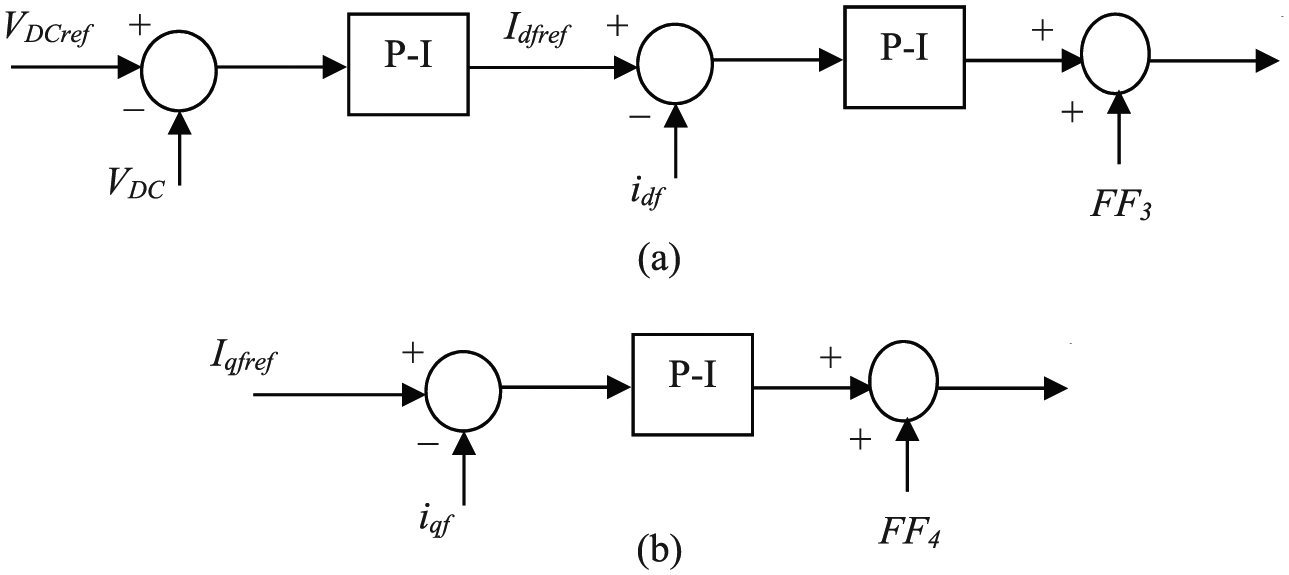
(a) d-axis control block of DFIG grid side converter and (b) q-axis control block of DFIG grid side converter.

GSC maintains the DC link voltage (V_DC) fixed at its reference value (V_DCref). The error signal of V_DC and V_DCref passes through a P-I controller to produce the d-axis current reference (I_dfref). The q-axis reference current depends on the value of the reactive power exchange between GSC and grid. The GSC d-axis and q-axis output currents (i_df and i_qf) are compared with the corresponding reference currents I_dfref and I_qfref, respectively, and the error signals pass through the P-I controllers to generate d-axis and q-axis reference voltages $v_{d f_{r e f}}$ and $v_{q f_{r e f}}$ . The expressions of the P-I controller parameters of Figure 3 are obtained using pole-zero cancellation as

K_{P d} = K_{P q} = \frac{L_{g}}{τ^{″}} and K_{I d} = K_{I q} = \frac{R_{g}}{τ^{″}}

(39)

Here, $τ^{″}$ is the time constant for the GSC current control loop.

As per the standard practice, the controller dynamics of the GSC are not considered in small signal stability study (Mitra and Chatterjee, 2016). This is because the GSC controller parameters (K_P and K_I) are not decided by the specific DFIG driven wind farm as can be seen from equation (51). The main function of the GSC controllers is to influence the DC link dynamics (Mitra and Chatterjee, 2016; Vittal and Ayyanar, 2013). On the contrary, RSC controller parameters (K_P and K_I) are specific to DFIG and are decided by the machine parameters as can be seen from equation (34). Hence, RSC controller dynamics are considered for the small signal stability study.

Pitch controller

The output power of DFIG is maintained at its rated value (P_rated) when the wind speed exceeds the rated speed (V_{w_rated}), because otherwise the machine may get damaged. Since the power is the product of torque and speed (P =T_e × ω_r), both T_e and ω_r are maintained at the respective rated value. The torque is kept equal to $T_{e_{r a t e d}}$ by making $T_{e_{r e f}} = T_{e_{r a t e d}}$ in the RSC control (Figure 2(a)). In order to maintain $ω_{r} = ω_{r_{r a t e d}}$ , pitch controller is used. The schematic diagram of the pitch controller is shown in Figure 4. It consists of a P-I controller, one actuator, a dead zone and a rate limiter (Vittal and Ayyanar, 2013). The reference pitch angle β_ref depends on the values of proportional gain K_{_ωr} and the integral time T_{_ωr} of the P-I controller. The actuator time constant is T_{_β}. The rate of change of pitch angle β is limited by a pitch rate limiter $({| d β / d t |}_{\max})$ and a dead zone $({| d β / d t |}_{\min})$ . The differential and algebraic equations representing the pitch controller of Figure 4 are as follows

\frac{d φ_{ω r}}{d t} = - \frac{1}{T_{ω r}} φ_{ω r} + \frac{1}{K_{ω r}} β_{r e f}

(40)

\frac{d β}{d t} = \frac{1}{T_{β}} (β_{r e f} - β)

(41)

β_{r e f} = (ω_{r_{r a t e d}} - ω_{r}) K_{ω r} + φ_{ω r} \frac{K_{ω r}}{T_{ω r}}

(42)

Here, ϕ_ωr and β are the state variables and β_ref is the pitch angle set point.

Figure 4.

Pitch controller.

Small signal model of the complete power system

Wind speed below the rated value

At first, the case with wind speed less than the rated value is considered. So the action of the pitch controller is not included. Linearizing equations (30) and (32) for the ith DFIG, we have

\frac{d Δ φ_{i d i}}{d t} = Δ I_{d r r e f i} - Δ i_{d r i}

(43)

\frac{d Δ φ_{i q i}}{d t} = Δ I_{q r r e f i} - Δ i_{q r i}

(44)

Here, Δi_dri and Δi_qri can be expressed in terms of $Δ {e^{'}}_{d i}$ , $Δ {e^{'}}_{q i}$ , Δi_dsi and Δi_qsi. Similarly, ΔI_drrefi and ΔI_qrrefi can be expressed in terms of the DFIG differential and algebraic variables.

Considering equations (8) to (14) and (43) and (44), for each i = n + 1, . . ., n + n_dg and writing in compact form

Δ {\overset{\cdot}{X}}_{d g i} = F_{1 i} Δ X_{d g i} + F_{2 i} Δ V_{l d g i} + F_{3 i} Δ Z_{d g i} + E_{2 i} Δ u_{d g i}

(45)

So, for all the n_dg number of DFIGs, equation (45) can be written as

Δ {\overset{\cdot}{X}}_{d g} = F_{1} Δ X_{d g} + F_{2} Δ V_{l d g} + F_{3} Δ Z_{d g} + E_{2} Δ u_{d g}

(46)

Equations for expressions of power exchanged by the DFIG with the system network can also be written in matrix form to get

\begin{array}{l} 0 = G_{1 i} Δ X_{d g i} + G_{2 i} Δ V_{g i} + G_{3 i} Δ V_{l i} + G_{4 i} Δ V_{l d g i} + G_{5 i} Δ Z_{d g i} + E_{3 i} Δ u_{d g i} \\ for i = n + 1, \dots, n + n_{d g} \end{array}

(47)

Considering n_dg number of DFIG, equation (47) can be written as

0 = G_{1} Δ X_{d g} + G_{2} Δ V_{g} + G_{3} Δ V_{l} + G_{4} Δ V_{l d g} + G_{5} Δ Z_{d g} + E_{3} Δ u_{d g}

(48)

Linearizing equations (31) and (33) for each i = n + 1, . . ., n + n_dg, we get

\begin{matrix} 0 = K_{P d i} (Δ I_{d r r e f i} - Δ i_{d r i}) + K_{I d i} Δ φ_{i d i} - ω_{r i} σ L_{r r i} Δ i_{q r} - i_{q r} σ_{i} L_{r r i} Δ ω_{r i} \\ - ω_{r i} \frac{L_{m i}}{L_{s s i}} Δ ψ_{q s i} - ψ_{q s i} \frac{L_{m i}}{L_{s s i}} Δ ω_{r i} - Δ v_{d r i} \end{matrix}

(49)

0 = K_{P q i} (Δ I_{q r r e f i} - Δ i_{q r i}) + K_{I q i} Δ φ_{i q i} - ω_{r i} σ_{i} L_{r r i} Δ i_{d r i} - i_{d r i} σ_{i} L_{r r i} Δ ω_{r i} - Δ v_{q r i}

(50)

Considering equations (49) and (50) for all n_dg number of DFIG and putting in compact form, we get

0 = S_{1} Δ X_{d g} + S_{2} Δ V_{l d g} + S_{3} Δ Z_{d g} + E_{4} Δ u_{d g}

(51)

Here, F₁, F₂, F₃, G₁, G₂, G₃, G₄, G₅, S₁, S₂, S₃, E₂, E₃ and E₄ are block diagonal matrices.

Equations (13) and (14) will be modified due to the introduction of the additional bus (wind farm terminal bus) as given below

0 = C_{1} Δ X + C_{2} Δ I_{g} + C_{3} Δ V_{g} + C_{4} Δ V_{l} + C_{5} Δ V_{l d g}

(52)

0 = D_{1} Δ V_{g} + D_{2} Δ V_{l} + D_{3} Δ V_{l d g}

(53)

Here, $X_{d g} = {[i_{d s} i_{q s} {e^{'}}_{d s} {e^{'}}_{q s} ω_{r} θ_{t w} ω_{t} ϕ_{d} ϕ_{q}]}^{T}$ ; $V_{g} = {[θ_{1} V_{1} \dots θ_{m} V_{m}]}^{T}$ ; $V_{l} = {[θ_{m + 1} V_{m + 1} \dots θ_{n} V_{n}]}^{T}$ ; Vldg = [θn+1 $V_{n + 1} \dots θ_{n + n_{d g}} V_{n + n_{d g}}]^{T}$ ; $Z_{d g} = {[v_{d r} v_{q r}]}^{T}$ ; $u_{d g} = {[u_{d g (n + 1)}^{T} \dots u_{d g (n + n_{d g})}^{T}]}^{T}$ , where $u_{d g i} = {[V_{w} T_{e_{r e f i}}]}^{T}$ .

The DFIGs are connected to load buses, so only the load flow Jacobian will change. Therefore, combining the equations (11) and (12), (46), (48), (51) to (53), the system equation in matrix form is given as

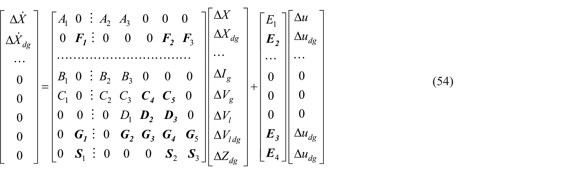
[\begin{matrix} Δ \overset{\cdot}{X} \\ Δ {\overset{\cdot}{X}}_{d g} \\ \dots \\ 0 \\ 0 \\ 0 \\ 0 \\ 0 \end{matrix}] = [\begin{array}{l} A_{1} & 0 & ⋮ & A_{2} & A_{3} & 0 & 0 & 0 \\ 0 & F_{1} & ⋮ & 0 & 0 & 0 & F_{2} & F_{3} \\ \dots & \dots & \dots & \dots & \dots & \dots & \dots & \dots \\ B_{1} & 0 & ⋮ & B_{2} & B_{3} & 0 & 0 & 0 \\ C_{1} & 0 & ⋮ & C_{2} & C_{3} & C_{4} & C_{5} & 0 \\ 0 & 0 & ⋮ & 0 & D_{1} & D_{2} & D_{3} & 0 \\ 0 & G_{1} & ⋮ & 0 & G_{2} & G_{3} & G_{4} & G_{5} \\ 0 & S_{1} & ⋮ & 0 & 0 & 0 & S_{2} & S_{3} \end{array}] [\begin{array}{l} Δ X \\ Δ X_{d g} \\ \dots \\ Δ I_{g} \\ Δ V_{g} \\ Δ V_{l} \\ Δ V_{l d g} \\ Δ Z_{d g} \end{array}] + [\begin{array}{l} E_{1} \\ E_{2} \\ \dots \\ 0 \\ 0 \\ 0 \\ E_{3} \\ E_{4} \end{array}] [\begin{array}{l} Δ u \\ Δ u_{d g} \\ \dots \\ 0 \\ 0 \\ 0 \\ Δ u_{d g} \\ Δ u_{d g} \end{array}]

(54)

The bold letters in equation (54) indicate the modified and/or new co-efficients added in equation (15). Equation (66) can be reduced as

Δ \overset{\cdot}{X^{'}} = {A^{'}}_{s y s} Δ X^{'} + E^{'} Δ u^{'}

(55)

where $Δ \overset{\cdot}{X^{'}} = {[Δ \overset{\cdot}{X} Δ {\overset{\cdot}{X}}_{d g}]}^{t}$ and the system matrix ${A^{'}}_{s y s} = \tilde{A} - \tilde{B} {\tilde{D}}^{- 1} \tilde{C}$ , where $\tilde{A} = [\begin{array}{l} A_{1} 0 \\ 0 F_{1} \end{array}]$ , $\tilde{B} = [\begin{array}{l} A_{2} A_{3} 0 0 0 \\ 0 0 0 F_{2} F_{3} \end{array}]$ , $\tilde{C} = [\begin{array}{l} B_{1} 0 \\ C_{1} 0 \\ 0 0 \\ 0 G_{1} \\ 0 S_{1} \end{array}]$ and $\tilde{D} = [\begin{array}{l} B_{2} B_{3} 0 0 0 \\ C_{2} C_{3} C_{4} C_{5} 0 \\ 0 D_{1} D_{2} D_{3} 0 \\ 0 G_{2} G_{3} G_{4} G_{5} \\ 0 0 0 S_{2} S_{3} \end{array}]$ .

Wind speed above the rated value

Next, we consider the condition of wind speed above the rated value. Here, the pitch controller equations are included. Using the linearized equations (8) to (14), (43) and (44), along with the linearized form of equations (40) and (41) and then writing in matrix form, we have

Δ {\overset{\cdot}{X}}_{d g} = F_{1} Δ X_{d g} + F_{2} Δ V_{l d g} + F_{3} Δ Z_{d g} + E_{2} Δ u_{d g}

(56)

The size of all the matrices will increase because of the introduction of two more linearized equations (equations (40) and (41)).

Linearized equations for power exchanged by DFIG with system network with modified X_dg can be written in matrix form (size of G₁ and E₃ will change), for all n_dg number of DFIG, we have

0 = G_{1} Δ X_{d g} + G_{2} Δ V_{g} + G_{3} Δ V_{l} + G_{4} Δ V_{l d g} + G_{5} Δ Z_{d g} + E_{3} Δ u_{d g}

(57)

Similarly, linearized equations (49) and (50) and the linearized form of equation (42) can be written in matrix form (size of S₁, S₂, S₃ and E₄ will change) for all n_dg number of DFIG as

0 = S_{1} Δ X_{d g} + S_{2} Δ V_{l d g} + S_{3} Δ Z_{d g} + E_{4} Δ u_{d g}

(58)

Here, F₁, F₂, F₃, G₁, G₂, G₃, G₄, G₅, S₁, S₂, S₃, E₂, E₃ and E₄ are block diagonal matrices.

The modified variables are

X_{d g} = {[\begin{matrix} i_{d s} & i_{q s} & {e^{'}}_{d s} & {e^{'}}_{q s} & ω_{r} & θ_{t w} & ω_{t} & ϕ_{d} & ϕ_{q} & ϕ_{ω r} & β \end{matrix}]}^{T}; u_{d g} = {[u_{d g (n + 1)}^{T} \dots u_{d g (n + n_{d g})}^{T}]}^{T}

where $u_{d g i} = {[V_{w} T_{e_{r e f i}} β_{r e f i}]}^{T}$ .

The system equation in matrix form can be obtained by combining equations (56) to (58). This compact matrix is similar to the one shown in equation (54) with few modifications in the co-efficient matrices F₁, F₂, F₃, G₁, S₁, S₂, S₃, E₂, E₃ and E₄. This equation again can be reduced as before to get ${A^{'}}_{s y s}$ matrix.

Result of small signal stability analysis

A DFIG-based wind farm of capacity 100 MW is considered to be connected at the load buses (one at a time) of WSCC 3-machine 9-bus system. The capacity of the wind farm is 100 MW and the system base is 100 MVA. The eigenvalues of the system matrix of the linearized model of the system are obtained. The real part of the eigenvalue is denoted by σ_e. The minimum of absolute value of real part of the eigenvalues of the A_sys matrix in the left half plane (abs(σ_{e_}_min)) provides a clear idea about the small signal stability margin of the power system in the presence of wind farm along with its controllers. The change of σ_{e_}_min with change of wind power penetration is shown in Table 1. It can be observed from the table that with the increase in the wind power penetration, σ_{e_}_min is shifted towards the imaginary axis when wind farm is present at bus 5. This indicates a decrease in system stability with increase in wind power at bus 5. On the contrary, σ_{e_}_min shifted away from the imaginary axis indicating an improvement in small signal stability of the system with increase in wind power when wind farm is connected at bus 8. So, depending on the wind farm location, variation of the system stability may behave differently along with wind power variation. Also, it may be observed that the dominating states change, with increase in wind power, corresponding to the eigenvalue with σ_e closest to the imaginary axis in the left half plane. For example, for wind farm at bus 5, when P_dg is 0.7 pu, the dominant states corresponding to the eigenvalue with σ_{e_}_min are ${e^{'}}_{d}$ and ${e^{'}}_{q}$ , whereas with P_dg equal to 0.9 pu, the dominant states become δ₂, ${e^{'}}_{d}$ and ${e^{'}}_{q}$ . Similarly, for wind farm at bus 8, the dominant states change from ( ${e^{'}}_{d}$ and ${e^{'}}_{q}$ ) to (δ₂, ${e^{'}}_{d}$ and ${e^{'}}_{q}$ ) when P_dg changes from 0.7 to 0.9 pu. One more thing that can be observed from Table 1 is that, for wind farm at bus 5, the position of the eigenvalue having σ_{e_}_min as its real part is relatively away (–0.085531 for P_dg = 0.5 pu) from the imaginary axis with respect to the case when wind farm is at bus 8 (–0.058367 for P_dg = 0.5 pu). However, with the increase in wind power, the stability deteriorates when wind farm is connected to bus 5 and stability improves with increase in wind power when wind farm is connected to bus 8 of the 9-bus system.

Table 1.

Variation of eigenvalue for different wind power penetration.

DFIG at (bus)	P_dg	Eigenvalue (σ_e closest to the imaginary axis in the left half plane)	Dominant states	σ_{e_} _min
5	0.5	−0.085531 ± j7.752693	${e^{'}}_{d}$ , ${e^{'}}_{q}$	−0.085531
	0.7	−0.085426 ± j7.752722	${e^{'}}_{d}$ , ${e^{'}}_{q}$	−0.085426
	0.9	−0.085217 ± j7.752841	δ₂, ${e^{'}}_{d}$ , ${e^{'}}_{q}$	−0.085217
	0.95	−0.085147 ± j7.752892	δ₂, ${e^{'}}_{d}$ , ${e^{'}}_{q}$	−0.085147
8	0.5	−0.058367 ± j6.534325	${e^{'}}_{d}$ , ${e^{'}}_{q}$	−0.058367
	0.7	−0.058371 ± j6.534326	${e^{'}}_{d}$ , ${e^{'}}_{q}$	−0.058371
	0.9	−0.058380 ± j6.534325	δ₂, ${e^{'}}_{d}$ , ${e^{'}}_{q}$	−0.058380
	0.95	−0.058384 ± j6.534323	δ₂, ${e^{'}}_{d}$ , ${e^{'}}_{q}$	−0.058384

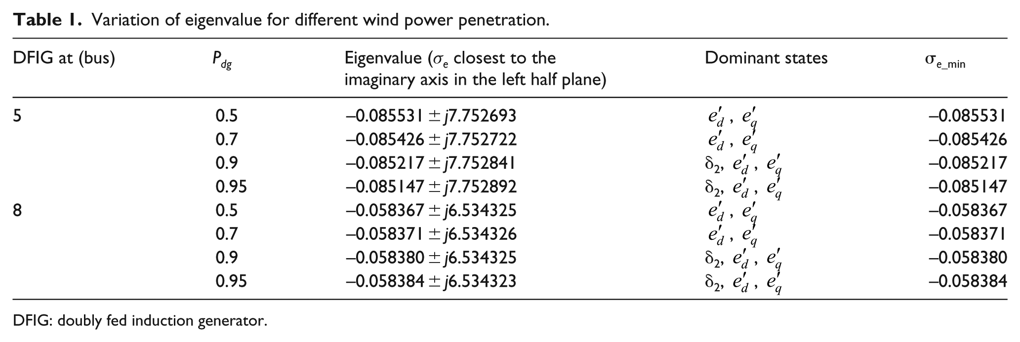
DFIG: doubly fed induction generator.

Calculation of proposed eigenvalue sensitivity

As shown from Table 1, the minimum of absolute values of real part of the eigenvalues in the left hand side of the imaginary axis (abs(σ_{e_}_min)) changes with increase in penetration. In case of wind farm connected to bus 8, σ_{e_}_min shifts away from the imaginary axis. However, if we are interested to know the limit of wind power penetration up to which the system remains stable, we have to keep on increasing the wind power and find σ_{e_}_min. Although the absolute value of σ_{e_}_min increases initially, at the point of instability, σ_{e_}_min has to become zero. So definitely, there will be point where absolute value of σ_{e_}_min will start decreasing. This point must be close to point of instability. One way to identify this point might be to compute eigenvalue sensitivity. The calculation of eigenvalue sensitivity is shown here.

Let ‘A’ be a function of system parameter α. Then, any eigenvalue λ_i of matrix Ã_sys is also a function of α, that is, λ_i(α), where i = 1, 2,. . ., n.

Let the parameter α change from α₀ to α₀ + ∆α, then, the corresponding change in system eigenvalue is from λ_i(α₀) to λ_i(α₀ + ∆α).

By Taylor series expansion and neglecting higher terms since ∆α is very small, we get

Δ λ_{i} (α_{0}, Δ α) = λ_{i} (α_{0} + Δ α) - λ_{i} (α_{0}) = \frac{\partial λ_{i} (α)}{\partial α} Δ α, at α = α_{0}

(59)

where ∂λ_i/∂α is the first-order sensitivity of eigenvalue λ_i to parameter α (Garmroodi et al., 2014; Gautam et al., 2009).

In this work, to find out the impact of increase in wind power on the system small signal stability, the sensitivity of σ_{e_}_min is calculated with respect to the change in P_dg. This is denoted by S_λ. The sensitivity is computed numerically by considering two very close points of P_dg (say P_dg₁ and P_dg₂) and the corresponding value of σ_{e_}_min, such that

S_{λ} = \frac{\partial σ_{e_\min}}{\partial P_{d g}} = \frac{Δ σ_{e_\min}}{Δ P_{d g}}

(60)

where ΔP_dg = P_dg₂ – P_dg₁ is the change in P_dg and Δσ_{e_}_min = σ_{e_}_min2 – σ_{e_}_min1 is the change in σ_{e_}_min.

Result with eigenvalue sensitivity

The eigenvalue sensitivity (S_{_λ}) is calculated using equation (60). The change in P_dg is taken here as 0.01 pu. The study is carried out in WSCC 3-machine 9-bus system and IEEE 16-machine 68-bus system.

Study in WSCC 3-machine 9-bus system

The wind farm is considered to be connected at one of the load buses (buses 5, 6 and 8). The capacity of the wind farm is 100 MW.

The effect of increase in wind power on the small signal stability is studied considering a particular wind speed. It is considered that the wind farm is capable of generating maximum power corresponding to that wind speed under rated condition.

At first, the wind farm is considered at bus 8 of the 9-bus system. The plot of variation of S_{_λ} with variation of the wind power penetration is shown in Figure 5(a). It can be observed that S_λ is positive and increasing with increase of penetration. This means minimum of the real part of all the eigenvalues moves away from the imaginary axis in the left half plane, thus indicating a more stable system. Similar plots for the wind farm at buses 5 and 6 are shown in Figure 5(b). It can be seen that S_{_λ} is negative and its value decreases with increase of P_dg, thus indicating movement of the minimum of the real part of the eigenvalues towards the imaginary axis. Hence, the small signal stability condition deteriorates with increased wind power injection at these buses. For wind farm capacity of 100 MW, the system stability gradually increases with increase in load. Let us now consider that the wind farm has a larger capacity (150 MW). The peak value of the sensitivity plot for this higher wind power penetration is found to be at P_dg = 1.23 pu (Figure 6). That is, S_{_λ} starts decreasing as P_dg increases beyond 1.23 pu (penetration = 28.1%). So for the 9-bus system, the optimum wind power penetration at bus 8 is 1.23 pu.

Figure 5.

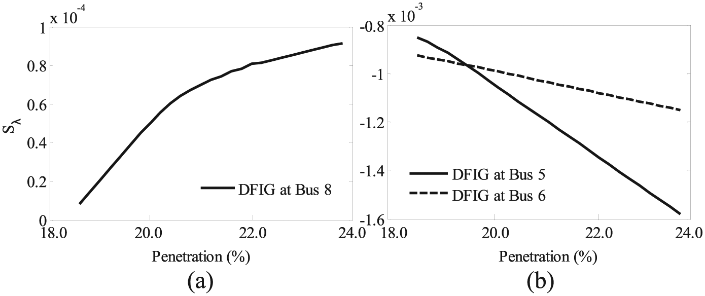
Variation of eigenvalue sensitivity (S_{_λ}) with wind power penetration for (a) DFIG at bus 8, and (b) DFIG at buses 5 and 6.

Figure 6.

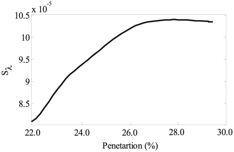
Variation of eigenvalue sensitivity (S_{_λ}) with wind power penetration for DFIG at bus 8.

Study in IEEE 16-machine 68-bus system

Different small groups of buses were considered as different zones (Kundur, 1994) as given below.

Zone I: 15, 16, 17, 18, 19, 20, 21, 22, 23, 24, 27, 56, 57, 58, 59

Zone II: 4, 5, 6, 7, 8, 9, 10, 11, 12, 13, 14, 54, 55

Zone III: 1, 2, 3, 17, 18, 25, 26, 27, 28, 29, 53, 60, 61

Zone IV: 1, 9, 30, 31, 32, 33, 34, 35, 36, 37, 62, 63, 64

Wind farm is considered to be connected at different load buses one at a time in each zone. The study is carried out in zone I by considering that wind power is available near the buses 15, 16 and 17, one at a time. The wind farm capacity is considered to be 1000 MW (obtained by aggregating 200 units of 5 MW each). The system base is considered to be 100 MVA. The reactive power exchange with the system is considered to be zero.

The variation of eigenvalue sensitivity with the variation in the wind power penetration can be observed in Figure 7 for the three different wind farm locations. It is observed that the sensitivity S_{_λ} increases with increase in penetration when the wind farm is at bus 16, indicating an improvement in system stability. When the wind farm is present at bus 15 or bus 17, S_{_λ} decreases with increase in wind power penetration indicating deterioration of the system small signal stability. 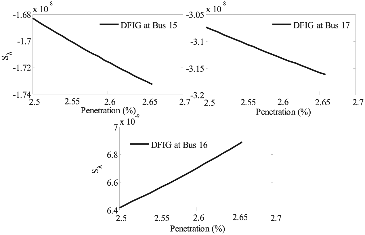The dominating state corresponding to the eigenvalue with σ_{e_}_min is the voltage behind the transient reactance of the synchronous generator 7 $({E^{'}}_{q 7})$ for wind farm at bus 15 and bus 17. For wind farm at bus 16, the dominating state is the exciter voltage of the synchronous generator 15 $(E_{f d 15})$ of the 68-bus system. For a larger capacity of wind farm (2000 MW), the optimum wind power penetration at bus 16 is found to be 19.05 pu (penetration = 9.46%). The corresponding plot of S_{_λ} with respect to the variation of wind power penetration is shown in Figure 8.

Figure 7.

Variation of eigenvalue sensitivity (S_{_λ}) with wind power penetration.

Figure 8.

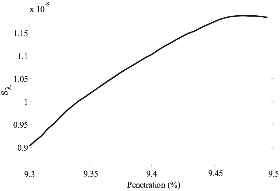
Variation of eigenvalue sensitivity (S_{_λ}) with wind power penetration for DFIG at bus 16.

Conclusion

The eigenvalue sensitivity analysis is carried out to find the impact of increase in wind power at the load bus where the wind farm is connected. It is observed that the impact on the small signal stability of the system with the variation of the wind power is location dependent. Moreover, the cases with which the stability improves with increase in wind power, there exists an optimum value exceeding which eigenvalue sensitivity decreases indicating deterioration of system stability. So with this study, the limit of wind power penetration at the system bus can be determined. One important point to be noted from the result shown is that this study of eigenvalues and the eigenvalue sensitivity gives an idea of location of wind farm suitable in terms of the inherent stability condition of the system (without application of any large disturbance).

Footnotes

Declaration of conflicting interests

The author(s) declared no potential conflicts of interest with respect to the research, authorship, and/or publication of this article.

Funding

The author(s) received no financial support for the research, authorship, and/or publication of this article.

ORCID iD

Arghya Mitra

References

Bianchi

Battista

Mantz

(2007) Wind Turbine Control Systems – Principles, Modelling and Gain Scheduling Design. London: Springer.

Wang

et al. (2012) Probabilistic analysis of small-signal stability of large-scale power systems as affected by penetration of wind generation. IEEE Transactions on Power Systems 27(2): 762–770.

Garmroodi

Hill

Jin

et al. (2014) Impact of wind generation variability on small signal stability of power systems. In: Australasian universities power engineering conference (AUPEC), Perth, WA, Australia, 28 September–1 October, pp. 1–6. New York: IEEE.

Gautam

Vittal

Harbour

(2009) Impact of increased penetration of DFIG-based wind turbine generators on transient and small signal stability of power systems. IEEE Transaction on Power Systems 24: 1426–1434.

Kundur

(1994) Power System Stability and Control. New York: McGraw-Hill.

Mei

Pal

(2007) Modal analysis of grid-connected doubly fed induction generators. IEEE Transactions on Energy Conversion 22(3): 728–736.

Mitra

Chatterjee

(2016) Active power control of DFIG-based wind farm for improvement of transient stability of power systems. IEEE Transactions on Power Systems 31(1): 82–93.

Nam

Kim

Shim

et al. (2000) A new eigen-sensitivity theory of augmented matrix and its applications to power system stability analysis. IEEE Transactions on Power Systems 15(1): 363–367.

Nolan

Sinha

Alden

RTH

(1976) Eigenvalue sensitivities of power systems including network and shaft dynamics. IEEE Transaction on Power Apparatus and Systems 95(4): 1318–1324.

10.

Nunes

MVA

Lopes

JAP

Zurn

et al. (2004) Influence of the variable-speed wind generators in transient stability margin of the conventional generators integrated in electrical grids. IEEE Transaction on Energy Conversion 19(4): 692–701.

11.

Vittal

Ayyanar

(2013) Grid Integration and Dynamic Impact of Wind Energy. New York: Springer.

12.

Wang

Shi

Wang

et al. (2008) Modelling analysis in power system small signal stability with grid-connected wind farms of DFIG type. Wind Engineering 32(3): 243–264.

13.

Wang

Chung

Tse

et al. (2000) Multimachine eigenvalue sensitivities of power system parameters. IEEE Transaction on Power Systems 15(2): 741–747.

14.

Yazdani

Iravani

(2010). Voltage-Sourced Converters in Power Systems Modeling, Control, and Application. Hoboken, NJ: John Wiley & Sons.