Adaptive filter–based power curve modeling to estimate wind turbine power output

Abstract

This article presents a comparative study of adaptive filter–based power curve models to estimate wind turbine power output. In the real world, wind turbines are never subjected to ideal conditions; thus, adaptive filter–based power curves serve best when estimating the power in a time-varying environment. Adaptive filter–based power curve is implemented using various algorithms like least mean square, kernel least mean square, recursive least square, and kernel recursive least square algorithms. All models have been developed on National Renewable Energy Laboratory datasets. The performance of various models has been compared on the basis of parameters like mean absolute error, root mean square error, and R-squared score. In addition to this, the learning curves of each method have been obtained to show the performance variation over time.

Keywords

Wind turbine power prediction online learning positive-definite kernel kernel least mean squares kernel recursive least squares learning curve

Introduction

To optimize the operational cost and improve the reliability of the wind energy power system, a reliable and accurate model for performance measurement of a wind turbine is required. In the wind energy industry, it is usually convenient to express the performance by power curve from which actual performance can be determined regardless of how the turbine is operated (Carrillo et al., 2013; Lydia et al., 2014). The power curve of the wind turbine establishes the relationship between wind speed and wind power. An ideal power curve is shown in the left panel of Figure 1. Ideal power curve gives a typical power extraction, but it cannot be valid for every model.

Figure 1.

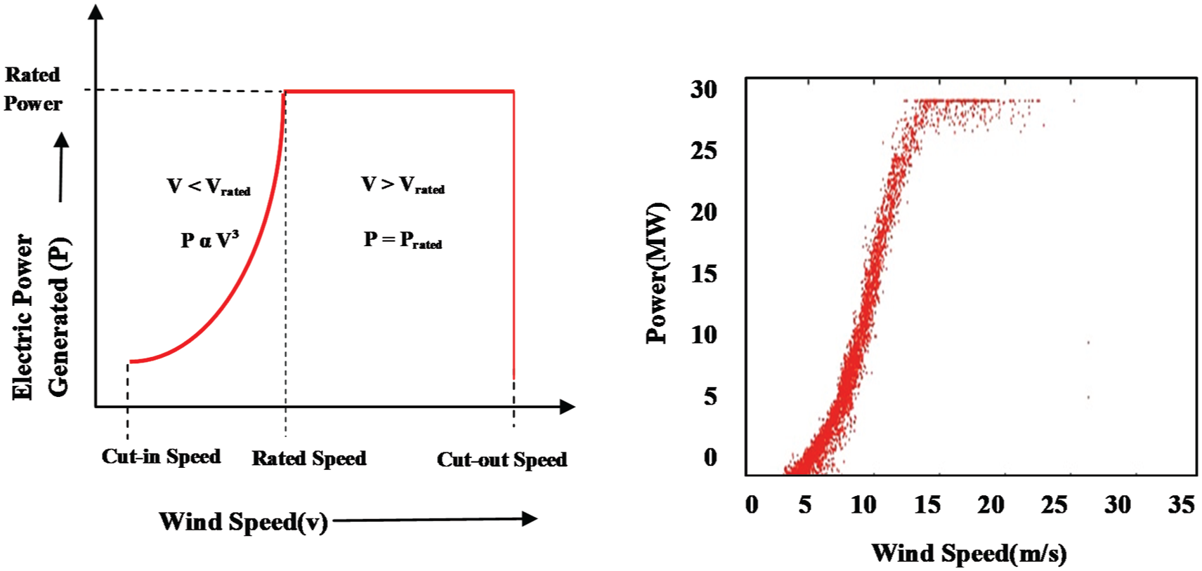
Left panel shows the ideal power curve and the right panel shows actual power production data plotted using NREL dataset.

Thapar et al. (2011) stated that commercially available wind turbines have their own design and rating that be a cause of the differences in the shape of their power curves. The actual power curve of the machine is supplied by the manufacturer, which characterizes the response of the machine, that is, the output that a wind turbine will produce at any given location, at particular wind speed. The actual power curve of the machine only considers the turbine design and rating; therefore, when installing at different customer sites, the actual power output of the turbine presents a more complicated picture. In the right panel of Figure 1, scatter plot has been used to show how much wind power is affected by wind speed. The data points provided in the resource file of National Renewable Energy Laboratory’s (NREL; 2012) HOMER software have been used for plotting. In this plotting, the hourly observations of the year 2012 are used. Previously, a number of studies were undertaken to develop the quality power curve to estimate the power production of wind turbine and some of them are reported in Kusiak et al. (2008), Li et al. (2001), Wadhvani et al. (2017), and Wan et al. (2014). Research started with various statistical models in which the power curve is obtained by using various parametric regression methods. Parametric regression method aims to estimate the target function of independent variables called the “regression function” which helps to characterize the variations of the dependent variable. In this method, for a known functional relationship between the dependent and independent variables, the parameters of the function are estimated, which best fits the observational data. Lydia et al. (2013), Shokrzadeh et al. (2014), and Wadhvani and Shukla (2018) have introduced various parametric regression techniques for power curve modeling, such as linearized segmented regression, four-parameter and five-parameter logistic regression, polynomial regression, spline regression, natural cubic spline regression, and locally weighted spline regression. Anyone of these can be used for curve fitting depending on the pattern of the data available for prediction. However, these models were restricted by their nature and did not solve the problem of nonlinearity in the datasets. To overcome these limitations and to enhance the accuracy and quality of the power curve, other popular data-driven methods include support vector machines (Zhu et al., 2013), neural networks (Morshedizadeh et al., 2017b), and fuzzy logics (Üstüntaş and Şahin, 2008). In their research, Morshedizadeh et al. (2017a) have preferred the combination of fuzzy logic and neural networks to model the power curve as they are able to precisely model a wide range of possible shapes of curves. Although the reported approaches improved the quality of the power curve, one of the limitations with these models is that they do not consider the dynamic behavior of the power curve. In view of the above limitation, researchers have observed that the properties of the power curve (i.e. shape and curvature) vary over time. Even in the small time domain, any change in weather conditions is immediately reflected in the properties of the curve. Recently, Lee et al. (2015) and Long et al. (2015) have proposed power curve modeling approaches to monitor the wind power generation performance by analyzing the variations of wind power curves over the time. In their research, multivariate approaches have been used to monitor multiple parameters simultaneously.

After several studies, it has been observed that the wind turbine may produce a different amount of power even if the wind speed is the same. The reason for the nonlinear relationship between wind speed and output power is the highly volatile and uncertain nature of wind. At different points of time, in dissimilar climate conditions, the status of the variables under study (i.e. wind speed and wind power) may change. For any change, if across new observations, the variance of the error term is not constant, then heteroscedasticity arise in time series data. In prediction, this type of predicament where heteroscedasticity occurs in observational data makes prediction a difficult task. For all these reasons, in power curve modeling, time-domain analysis of observational data is required, which is able to predict the power with varying residual error. Use of adaptive filters in prediction can be a solution to the problem. Earlier applications of adaptive filters were limited to signal processing, channel equalization and identification, adaptive feedback cancelation, signal control, prediction, and so on. Prapulla et al. (2008) have proposed the least mean square (LMS) adaptation technique for equalization of $π / 4$ –differential quadrature phase shift keying ( $π / 4$ -DQPSK) signals and achieved outstanding performance. This article extends the use of adaptive filters for estimating wind power generation because adaptive filters serve best when applied in a time-varying environment. This feature of the adaptive filter is known as online adaptation. “Adaptive filter–based power curve modeling” section of this article describes two linear online adaption techniques: Least Mean Square (LMS) algorithm and Recursive Least Square (RLS) algorithm. Also, the nonlinear variants of LMS and RLS, that is, Kernel Least Mean Squares (KLMS) and Kernel Recursive Least Squares (KRLS), respectively, have been introduced.

Adaptive filter–based power curve modeling

An adaptive filter is a data-processing device that enables to find the time-varying input–output relationship in an iterative manner. As in Arora and Wadhvani (2017) and Clarkson (1993), an adaptive filter can be understood and defined via four basic features: the input signal to the filter, the filter structure, the structure parameters, and the adaptive algorithm. The filter structure of an adaptive filter defines the filter input–output relationship. Each adaptive filter consists of different sets of structure parameters which change themselves with every iteration in order to re-calibrate the filters’ input–output relationship. When a specific filtering structure is selected, the number and type of parameters associated with it can be modified as per requirement. Finally, the adaptive algorithm describes how the parameters will adjust or update themselves over time. The adaptive algorithm is also used as a form of an optimizer that minimizes the error for a particular dataset. Proper selection of structure parameters and adaptation algorithms is an utmost important task while implementing an adaptive filter. Typically, the parameters of the filter structure are updated through a process of sequential learning where data are available with time, usually one at a time. One of the problems with sequential learning is that it is more computationally intensive as it uses every training data for the adaption process. An alternative to this can be active learning, which uses a subset of informative training data for the adaption process. Consequently, active learning can significantly reduce the computational complexity with equivalent performance.

In order to capture the relationship between input and output variables, adaptive filters can be categorized into two ways: linear adaptive filters and nonlinear adaptive filters. Linear adaptive filter builds a linear relationship between input and output signal while the nonlinear adaptive filter builds the same relationship by projecting the input data to higher dimensional feature space and then estimating the filter parameters. The linear adaptive filter is shown in the left panel of Figure 2, where linear sequential learning updates the structure parameters in response to change in statistical variations in the filter structure in which the filter operates. 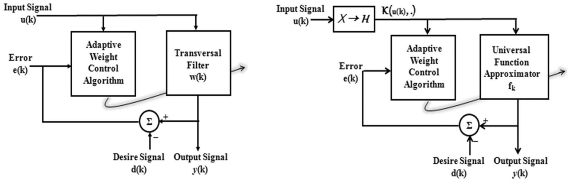The linear filter comprises a set of adjustable parameters denoted by $\vec{w}$ . For any given training examples ${u (1), d (1)}, {u (2), d (2)}, \dots\dots, {u (k), d (k)},$ after consuming k – 1 training samples, u(k) is current input signal, d(k) is the desired signal, y(k) is the actual output of filter, and e(k) is the error between desired and actual output. The current input u(k) and obtained error e(k) are then used to update the previous filter parameter, that is, $\vec{w} (k - 1)$ , by an incremental amount denoted by ∆w(k). So the update parameter vector of the filter becomes $\vec{w} (k) = \vec{w} (k - 1) + Δ w (k)$ . This process is continued till the filter parameter reaches a condition, whereafter the parameter adjustments become small enough to stop the adaptation.

Figure 2.

The left panel shows the linear adaptive filter and the right panel shows the nonlinear adaptive filter.

In the right panel of Figure 2, the elementary structure of the nonlinear adaptive filter is shown. Here, u(k) is input, d(k) is desired output, y(k) is actual output, and $f_{k}$ denotes nonlinear filter parameters. Here, input data are mapped to higher dimensional feature space using appropriate kernel methods, and then the filters adjust their parameters if error e(k) between the actual and the desired output is more than a predefined threshold value. As a nonlinear transfer function is implemented using the kennel method, therefore, this filter is also known as Kernel Adaptive Filter (KAF). In Kivinen et al. (2004) and Singh et al. (2012), the author has proposed KAF as an accurate learning method for nonlinear function, which performs sample by sample update via stochastic gradient-based method under universal approximation and convex optimization. The adaptation process makes use of online learning on a sequence of data samples recorded in a timely manner. In this modeling technique, initially for a given pair of input–output data points, the aim is to find out the relationship between the input and the output variables. The arrival of new data points may update this relationship. KAF naturally creates a growing radial basis function, learning the network topology and adapting its free parameters directly from data. KAF implements a nonlinear transfer function using kernel method. The use of kernels is introduced to transform certain classes of nonlinear tasks to equivalent linear ones. In these methods, the function is mapped to a high-dimensional feature space, even infinite-dimensional space, via a Mercer kernel. A Mercer kernel (Aronszajn, 1950) is a continuous, symmetric, positive-definite function К defined on X × X, where X € Rp $X € R^{p}$ denote a real-valued random input vector. Mercer had used the term positive-definite kernel to characterize the function of two points $К (u, d), u, d R^{p}$ and the corresponding space of functions, Η_k, which is generated by the linear span of ${К (\cdot, d), d € R^{p}}$ , that is, arbitrary linear combinations of form $f (x) = \sum_{m} a_{m} К (u, d_{m})$ , where each kernel term is viewed as a function of the first argument, and indexed by the second. Suppose that К has an eigen-expansion

К (u, d) = \sum_{i = 1}^{\infty} γ_{i} φ_{i} (u) φ_{i} (d)

(1)

with $γ_{i} > 0, \sum_{i = 1}^{\infty} γ_{i}^{2} < \infty$ . Elements of Η_k have an expansion in terms of these eigen functions

f (x) = \sum_{i = 1}^{\infty} c_{i} φ_{i} (u)

(2)

with the constraint that

{‖ f ‖}_{H_{k}}^{2} = \sum_{i = 1}^{\infty} \frac{c_{i}^{2}}{γ_{i}} < \infty

(3)

where ${‖ f ‖}_{H_{k}}$ is the norm induced by К. The most widely used reproducing kernels defined on X × X, with kernel width $(σ),$ is given in Table 1.

Table 1.

List of kernel functions applied in experiments.

Kernel function
Gaussian Kernel	$К_{σ} (u, d) = \exp (- \frac{‖ u - d ‖^{2}}{2 σ^{2}})$
Gauss–Aniso	$g_{o} (u, d; σ) = \frac{1}{2 π σ^{2}} e x p {- \frac{1}{2} (\frac{u^{2} + d^{2}}{σ^{2}})}$
The Laplacian kernel	$К_{t} (u, d) = e x p (- t \| \| u - d \| \|)$

In view of the fact that high-dimensional feature space is linear, KAFs can be thought of as a generalization of linear adaptive filters. Two popular algorithms, namely, LMS and RLS, have been used to update the structure coefficients of linear adaptive filters. The kernelized variants of LMS and RLS algorithms for weight updation of structure coefficients of nonlinear adaptive filters are KLMS and KRLS, respectively. They use kernel trick for mapping input data into a high-dimensional feature space, which is summarized in Liu et al. (2010).

LMS algorithm

The LMS algorithm is a class of linear adaptive algorithms.This algorithm updates the filter structure coefficients after evaluating the minimum mean square of the error signal. In general, the LMS algorithm performs two basic processes: the filtering process and the adaptive process. Role of the filtering process is to compute the output signal of the filter in accordance with input signals. Once the output signal is generated, it is then compared with the desired response to estimate net error. The aim is to automatically adjust the coefficients of the parameters in accordance with the estimated error. In all iterations of LMS algorithm, instantaneous value of squared estimation error, that is, $J (k) = 1 / 2 e^{2} (k)$ , is minimized, where k is a discrete time unit. The following operations are performed to update the coefficients of an adaptive filter:

Calculates the output signal, that is, $y (k) = w^{T} (k - 1) u (k)$ , from the adaptive filter.

Calculates the error signal, $e (k) = d (k) - y (k)$ .

Updates the filter coefficients by using the equation $\vec{w} (k) = \vec{w} (k - 1) + μ \cdot e (k) \cdot \vec{u} (k)$ .

where $\vec{u} (k)$ is the filter input vector, $\vec{w} (k)$ and $\vec{w} (k - 1)$ are the filter coefficients vector at instance k and k – 1, respectively, and µ is the step size of the adaptive filter. The value of µ determines how close our algorithm has converged toward the solution. Inverse relation exists between the convergence factor µ and the minimal error. An upper bound and lower bound is given to step size µ and is called the condition of convergence, defined as follows

0 < μ < \frac{1}{λ_{\max}}

(4)

where $λ_{\max}$ is the largest eigen value of the correlation matrix $R_{u}$ , defined by

R_{u} = \sum_{i = 1}^{N} \vec{u} (k) {\vec{u}}^{T} (k)

(5)

Also, the trace of the correlation matrix can be taken as a good estimate of $λ_{\max}$ and the condition can be given as

0 < μ < \frac{2}{t r [R_{u}]}

(6)

The choice of µ is the deciding factor for calculating the convergence speed. When µ is small, then convergence takes slowly, whereas for a larger value of μ, fast convergence of the algorithm is seen. However, the LMS algorithm is easily affected whenever its inputs are calibrated. This causes difficulty in choosing appropriate learning rate µ.

KLMS algorithm

KLMS is nothing but the radial basis function with the different assignment of centers and different training procedure. Each input data point is taken into consideration to obtain the results. This leads to an increase in memory and computational requirements. In Liu et al. (2008), the author has explained learning of KLMS as the LMS performed on the example sequence at time instance k, $f {φ (k), y (k)}$ . The kernel induces mapping to transform the data u(k) into the feature space F as $φ (u (k))$ which is interpreted as the usual dot product. This procedure is summarized as follows

\begin{array}{l} w (0) = 0 \\ y (k) = w {(k - 1)}^{T} φ (k) \\ e (k) = d (k) - w {(k - 1)}^{T} φ (k) \end{array}

(7)

where e(k) represents the error which is the difference of actual value, d(k), and the predicted value, $y (k),$ that is, $f_{k}$ at time instance k. In the above equation, for simplicity, φ(u(k)) is denoted by φ(k). The basic motive behind KAF is to optimize the filter weights, by updating the weights in a manner to converge to the optimal weights. The basic weights update equation based on stochastic gradient given as

w (k) = w (k - 1) + η e (k) φ (k)

(8)

When new training data come in with the input u(k) as the center and the difference between the predicted and the actual output as the coefficient $μ_{i}$ , a new kernel unit is allocated which is used by KLMS to finally update the model as follows

f_{k} = f_{k - 1} + η e (k) κ (u (k), .)

(9)

Kernel adaptive filtering algorithm has the limitation of the linearly growing structure with the input, which leads to an increase in memory and computational requirements. To deal with this problem, Vaerenbergh and Santamaria (2013) have applied different sparcification methods for taking only important input data as new centers. There are two versions of KLMS, namely, naïve online regularized risk minimization algorithm (NORMA) and quantized kernel least mean squares (QKLMS). NORMA is a KLMS algorithm with regularization that adds a penalty term to overcome the problem of over-fitting by reducing the importance given to noisy data. This algorithm uses a sliding-window dictionary mechanism in which it discards the oldest data points after certain iterations. In QKLMS algorithm, the dictionary is constructed by process of quantization to compress the feature space by reducing the number of centers in radial basis function, due to which network size and hardware complexity are reduced. In this method, redundant data are used to update the coefficient of the closest center. QKLMS does not include regularization since it has self-regularization property.

RLS algorithm

RLS is a class of adaptive filter which recursively updates the model coefficients relating to the input data point. The algorithm works best in time-varying or the non-stationary environment; however, it has higher computational complexity and low stability. The objective of the algorithm is the minimization of the sum of squared approximation errors up to the current time k. Along with this, a weighting factor is introduced in the cost function to ensure that less weight is assigned to earlier error samples so that statistical variations in the dataset can be identified more efficiently when the filter operates in the non-stationary conditions (Marshall et al., 1989). In all iterations of RLS algorithm, sum of squared estimation error, that is, $J (k) = \sum_{i = 1}^{k} β (k, i) e^{2} (k)$ , is minimized, where weighting factor β has the property $0 < β \leq 1$ for $i = 1, 2, \dots k$ . In literature, exponential weighting or forgetting factor has been applied as a common weighting strategy. It is defined as $β (k, i) = λ^{k - i}$ for $i = 1, 2, \dots k$ where λ is a positive constant, $0 < λ < 1$ . The solution of this problem is given as

w (k) = {U (k) U {(k)}^{T}}^{- 1} U (k) d (k)

(10)

where $w (k)$ is the filter parameter at time instance $k$ , $U (k)$ is the matrix containing input observations up to time instance $k$ , and $d (k)$ is the output vector at time instance $k$ .

Defining the matrix $P (k)$ as ${U (k) U {(k)}^{T}}^{- 1}$ and using matrix inversion lemma, $P (k)$ can be expressed as

P (k) = P (k - 1) - \frac{P (k - 1) u (k) u {(k)}^{T} P (k - 1)}{1 + u {(k)}^{T} P (k - 1) u (k)}

(11)

Finally, $w (k)$ can be defined directly from previous estimate $w (k - 1)$ as

w (k) = w (k - 1) + \frac{P (k - 1) u (k)}{1 + u {(k)}^{T} P (k - 1) u (k)} [d (k) - u {(k)}^{T} w (k - 1)]

(12)

During its execution, this algorithm consumes previous samples of error signals, output signals, and filter weights, hence requiring higher memory configuration. Another prominent feature of the RLS algorithm is that, while realization, this algorithm uniformly distributes its computation load in each iteration. However, one of the limitations with the algorithm is that it is not suitable for online filtering due to time-consuming computations of inverse matrix least squares methods.

KRLS algorithm

KRLS algorithm applies kernel trick to transform the input data u(i) into the feature space Z as φ(u(i)). This can be simply denoted as φ(i). Here, feature space is a high-dimensional space; thus, regularization is required. As in Liu et al. (2010), the weighted cost function for KRLS can be defined as

\min_{w} = \sum_{k = 1}^{i} β^{i - k} {| d (k) - w^{T} φ (k) |}^{2} + λ {‖ w ‖}^{2}

(13)

The normal form for weights can be defined as $w (i) = {[λ I + φ (i) φ {(i)}^{T}]}^{- 1} φ (i) d (i)$ . Using matrix inversion lemma and basic matrix properties, $w (i)$ can be written as $w (i) = φ (i) {[λ I + φ {(i)}^{T} φ (i)]}^{- 1} d (i)$ . Denoting $Q (i) = {[λ I + φ {(i)}^{T} φ (i)]}^{- 1}$ , $h (i) = φ {(i - 1)}^{T} φ (i)$ , and $a (i) = Q (i) d (i)$ . The prediction error $e (i)$ can be computed as $e (i) = d (i) - l_{i - 1} (u (i))$ , where $l_{i - 1} (u (i)) = \sum_{j = 1}^{i - 1} a_{j} (i - 1) k (u (j), u (j))$ . Here $a_{j} (i - 1)$ is the jth component of $a (i - 1)$ and $k$ is the kernel function. Finally, $w (i)$ can be estimated from $w (i - 1)$ as

\begin{array}{l} w (i) = w (i - 1) + m {(i)}^{- 1} [k (u (i), .) - \sum_{j = 1}^{i - 1} z_{j} (i) k (u (j), .)] e (i) \\ z (i) = Q (i - 1) h (i) \\ m (i) = λ + φ {(i)}^{T} φ (i) - z {(i)}^{T} h (i) \end{array}

(14)

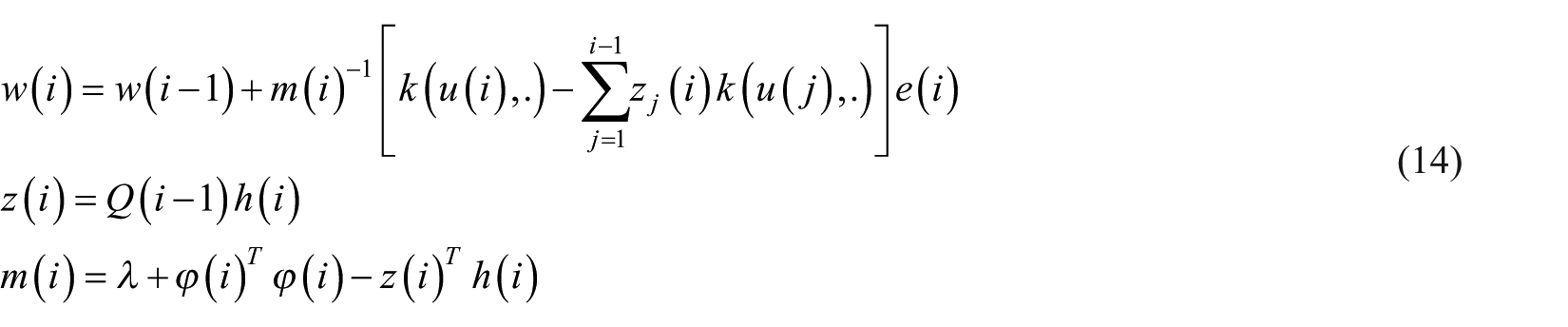
KRLS updates all the previous coefficients while KLMS never updates previous coefficients. The time and space complexity of KRLS is $O {(i)}^{2}$ , where i is the number of inputs till current time instance.

Real data application

In order to evaluate the performance of all the algorithms discussed in “Adaptive filter–based power curve modeling” section, a case study that includes the real data of the wind farms in North America is presented. For experimental purpose, two datasets are taken from the resource file of NREL, which specializes in renewable energy efficiency, research, and development. Datasets A and B correspond to site-id A 124693 and site-id B126541 (NREL, 2012), respectively. The geographical location of the site-id A is longitude −120.005463 and latitude 46.901657 with an average wind speed of 6.744 m/s. Site-id B has longitude −123.375778 and latitude 48.64072 with an average wind speed of 5.296 m/s. NREL obtained all these observations from SCADA (supervisory control and data acquisition) system’s wind plant. There are more than 1 lakh data observations recorded from January 2012 to December 2012. Usually, data collection methods are loosely controlled, resulting in out of range values (e.g. data points with negative wind power values), inconsistent data combination (e.g. data points with high wind speed and low power values, data points with low wind speed and high power values), missing values, and so on. Empirical power curve fitting to the data that have not been carefully scrutinized for such problems can produce misleading results. Before any modeling is taken up, data should be pre-processed. In order to pre-process raw data, an outlier detection method similar to Warren et al. (2011) has been applied. Here, each input observation that assumed to come with known data distribution is fitted with an elliptic envelope, in which only those power values that stand at most three standard deviations away from the mean of the distribution are allowed. A Mahalanobis distance metric is the well-known formula for measuring such type of distances. Before applying the above strategy to pre-process the datasets, datasets are divided into subparts, as the data observations over the period of one complete year show the nonlinear wind–power relationship and do not follow a normal distribution. The subparts are assumed to be normally distributed, pre-processed one by one and, at last, merged together to form cleaned nonlinear dataset. Figure 3 shows the plot of the wind speed and the output power for dataset over a 1-month period in March 2012 with the fitted decision boundaries using Mahalanobis distance metric. Once both the datasets are cleaned, they can be used to assess the performance of an adaptive filter.

Figure 3.

The scatter plot of the wind speed and the output power over a 1-month period in March 2012 with the fitted decision boundaries using Mahalanobis distance metric using dataset A.

The developed model characterizes the pattern of the actual data. To evaluate the ability of the model to generalize is important. Hence, parameters are required that evaluate the model on the basis of goodness of fit. The goodness of fit of the model can be decided by the loss function that judges the difference between estimated and true value. As in Kohavi (1995), mean square error (MSE), root mean square error (RMSE), and mean average error (MAE) have been applied as a loss function for measuring errors between desire output $d_{i}$ and predicted output $y_{i}$ . The mathematical expressions for MSE, MAE, and RMSE are given by

MSE = \frac{1}{k} \sum_{i = 1}^{k} {[y_{i} - d_{i}]}^{2}

(15)

MAE = \frac{1}{k} \sum_{i = 1}^{k} (| y_{i} - d_{i} |)

(16)

RMSE = \sqrt{\frac{1}{k} {(\sum_{i = 1}^{k} y_{i} - d_{i})}^{2}}

(17)

where $d_{i}$ is the observed wind power and $y_{i}$ is the predicted wind power using the realized model. These metrics come under the goodness of fit statistics; here, a value closer to zero indicates a better fit. On the contrary, how closely our model fits a particular dataset is determined by the coefficient of determination (R²). Value of R² score lies between 0 and 1. Zero value of R² score means that the response variable does not move around its mean. On the contrary, when R² score value tends to 1, it states that the relationship between our model and response variable is really strong. The mathematical expressions for R² score is given by

R^{2} = 1 - \frac{{\sum_{i = 1}^{k} (y_{i} - d_{i})}^{2}}{{\sum_{i = 1}^{n} (y_{i} - y_{i m})}^{2}}

(18)

here $y_{i m}$ is the mean of actual wind power for k samples.The performance of the proposed methodology has been validated in several ways. The performance of different modeling techniques can be compared on the basis of their learning curves depicting regression error over the period of time. Learning curves for different algorithms, namely, LMS, KLMS, RLS, and KRLS, have been obtained by a single run over the data, as shown in Figure 4, where MSE metric as in equation (15) has been used as a measure of regression error, which estimates the standard deviation of the random component in the data. To show the performance of the different methods in a comprehensive way, normalized MSE has been plotted. For the initial set of parameters in each experiment, this work relied on the cross-validation technique as described in Kohavi (1995). From the results generated, the algorithm-specific parameters were set as follows. For dataset A, LMS uses learning rate (step size), µ = 0.0001, KLMS uses learning rate or step size parameter, µ = 0.1, along with Gaussian kernel with the kernel parameter $σ = 0.1$ , RLS with forgetting factor, µ = 0.9966, and finally KRLS uses regularization parameter, µ = 0.5, along with Gaussian kernel with the kernel parameter σ = 1. For dataset B, LMS uses learning rate (step size), µ = 0.0001, KLMS uses learning rate or step size parameter, µ = 0.1, along with Gaussian kernel with the kernel parameter σ = 0.1, RLS with forgetting factor, µ = 0.9966, and finally KRLS uses regularization parameter, µ = 0.1, along with Gaussian kernel with the kernel parameter σ = 1. Initial weights for LMS and RLS have been initialized to zero values in both datasets.

Figure 4.

The left panel, middle panel, and right panel show the MSE performance comparison of LMS and RLS algorithms, LMS and KLMS algorithms, and RLS and KLS algorithms, respectively, on the basis of their learning curves using dataset A.

While investigating the left panel of Figure 4, it can be observed that compared to LMS, RLS algorithm shows reasonably fast convergence and the error rate decreases along with iterations. The error rate for RLS is comparatively lower than LMS as the number of iteration proceeds. While comparing LMS and KLMS in the middle panel of Figure 4, initially, the LMS algorithm starts with low error rate compared to KLMS, but after some iterations, KLMS experiences a steep decline in error rate and outperforms in convergence criteria. However, KLMS is computationally intensive, as for each training observation, a new kernel element is allocated. Finally, comparing RLS and KRLS plot in the right panel of Figure 4, for initial iterations, KRLS proceeds with large errors while RLS proceeds with low error values. However, similar to the LMS and KLMS plots, there is a steep descent in the KRLS curve while RLS slowly converges to minimum error values. After some point, KRLS attains a constant curve close to 0. This shows the convergence rate of KRLS is much faster than RLS, but the computational complexity of KRLS is much higher than RLS as KRLS takes into account the previous weights and inputs which have been processed so far. However, the forgetting factor determines how much weight should be given to past values.

Datasets A and B are also evaluated on the basis of MAE, RMSE, and R² score, as shown in Tables 2 and 3, respectively. From Table 2 for dataset A, it clearly shows that KRLS shows the least values for RMSE with highest R² score and have secured a position of 1 among all adaptive filters discussed above. The highest R² score of KRLS indicates that KRLS algorithm was able to fit dataset as close as possible to observed values. KLMS acquired a second slot with second highest R² score and with lowest MAE indicating a closer fit to the actual model. LMS and RLS perform nearly the same as their MAE, RMSE, and R² scores are close enough, and both have secured a position of 4 and 3, respectively.

Table 2.

MAE, RMSE, and R² score of various adaptive algorithms for dataset A.

S. No	Algorithm	µ	MAE	RMSE	R ²	Rank
1	LMS	0.0001	2.0064	2.2442	0.8508	4
2	RLS	0.9966	1.9418	2.1749	0.8599	3
3	KLMS	0.1000	0.0478	0.2422	0.9979	2
4	KRLS	0.5000	0.0574	0.2112	0.9984	1

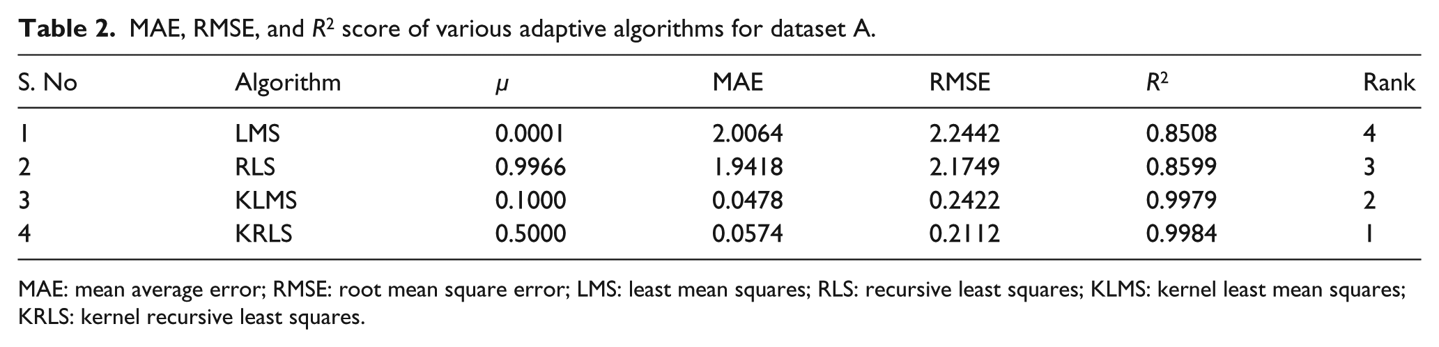
MAE: mean average error; RMSE: root mean square error; LMS: least mean squares; RLS: recursive least squares; KLMS: kernel least mean squares; KRLS: kernel recursive least squares.

From Table 3, it is clearly shown that KRLS shows the least values for MAE and RMSE with highest R² score and have secured a position of 1 among all adaptive filters discussed above. However, the regularization parameter is further tuned to achieve better results. KLMS again secured a second slot with second highest R² score. Good R² score indicates a closer fit to the actual model, and hence, KRLS and KLMS produced excellent results. LMS and RLS again produced a poor fit on the dataset. MAE, RMSE, and R² score for LMS and RLS were comparatively low with their kernel version, and both have again secured ranks 4 and 3, respectively.

Table 3.

MAE, RMSE, and R² score of various adaptive algorithms for dataset B.

S. No	Algorithm	µ	MAE	RMSE	R ²	Rank
1	LMS	0.0001	2.0613	2.2749	0.6701	4
2	RLS	0.9966	1.9356	2.2046	0.6901	3
3	KLMS	0.1000	0.1299	0.2971	0.9961	2
4	KRLS	0.1000	0.0432	0.0707	0.9997	1

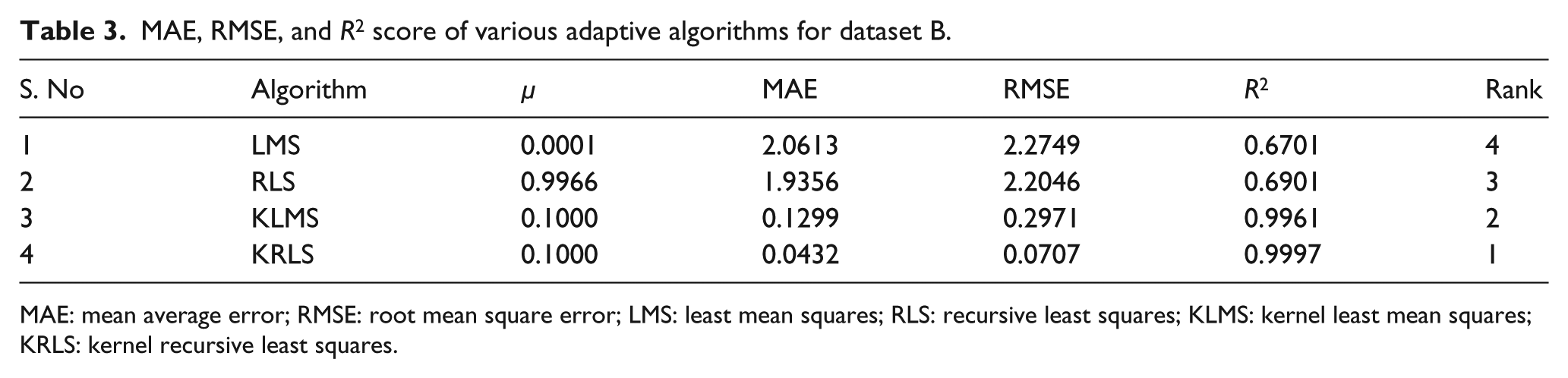
MAE: mean average error; RMSE: root mean square error; LMS: least mean squares; RLS: recursive least squares; KLMS: kernel least mean squares; KRLS: kernel recursive least squares.

Conclusion

Real wind power systems work under variable environmental conditions. To estimate the power production of such systems, this work presents a nonlinear model for power prediction. Two popular kernel-based adaptive learning approaches, that is, KLMS and KRLS, are applied to model the nonlinear power curve. The KLMS family is simple and computationally efficient. In contrast, KRLS family has the ability to adapt nonlinearity to a greater degree and thus provides a reasonably fast rate of convergence. Learning curves obtained for the different algorithms, that is, LMS, RLS, KLMS, and KRLS, have been analyzed on the basis of their MSE performance. Here, KRLS algorithm shows reasonable fast convergence on benchmark datasets. The performance achieved can be further improved by applying advanced sequential modeling approaches like recurrent neural network and their variants. These approaches have very low convergence rate for a specific dataset but perform optimally on the global scale.

Footnotes

Declaration of conflicting interests

The author(s) declared no potential conflicts of interest with respect to the research, authorship, and/or publication of this article.

Funding

The author(s) received no financial support for the research, authorship, and/or publication of this article.

ORCID iD

Bharti Dongre

References

Aronszajn

(1950) Theory of reproducing kernels. Transactions of the American Mathematical Society 68(3): 337–337.

Arora

Wadhvani

(2017) Comparative analysis of adaptive filters for predicting wind-power generation (SLMS, NLMS, SGDLMS, WLMS, RLMS). Intelligent Systems Design and Applications 736: 858–867.

Carrillo

Obando Montaño

Cidrás

(2013) Review of power curve modelling for wind turbines. Renewable and Sustainable Energy Reviews 21: 572–581.

Clarkson

(1993) Optimal and Adaptive Signal Processing. Boca Raton, FL: CRC Press.

Kivinen

Smola

Williamson

(2004) Online learning with kernels. IEEE Transactions on Signal Process 52(8): 2165–2176.

Kohavi

(1995) A study of cross-validation and bootstrap for accuracy estimation and model selection. In: Proceedings of the 14th international joint conference on artificial intelligence, vol. 2, Montreal, QC, Canada, 20–25 August, pp. 1137–1143. New York: Association for Computing Machinery.

Kusiak

Zheng

Song

(2008) Wind farm power prediction: a data-mining approach. Wind Energy 12(3): 275–293.

Lee

Ding

Genton

(2015) Power curve estimation with multivariate environmental factors for inland and offshore wind farms. Journal of the American Statistical Association 110(509): 56–67.

Wunsch

O’Hair

(2001) Using neural networks to estimate wind turbine power generation. IEEE Transactions on Energy Conversion 16(3): 276–282.

10.

Liu

Pokharel

Principe

(2008) The kernel least-mean-square algorithm. IEEE Transactions on Signal Processing 56(2): 543–554.

11.

Liu

Príncipe

Haykin

(2010) Kernel Adaptive Filtering: A Comprehensive Introduction. Hoboken, NJ: John Wiley.

12.

Long

Wang

Zhang

(2015) Data-driven wind turbine power generation performance monitoring. IEEE Transactions on Industrial Electronics 62(10): 6627–6635.

13.

Lydia

Kumar

Selvakumar

(2014) A comprehensive review on wind turbine power curve modeling techniques. Renewable and Sustainable Energy Reviews 30: 452–460.

14.

Lydia

Selvakumar

Kumar

(2013) Advanced algorithms for wind turbine power curve modeling. IEEE Transactions on Sustainable Energy 4(3): 827–835.

15.

Marshall

Jenkins

Murphy

(1989) The use of orthogonal transforms for improving performance of adaptive filters. IEEE Transactions on Circuits and Systems 36: 474–485.

16.

Morshedizadeh

Kordestani

Carriveau

(2017a) Application of imputation techniques and Adaptive Neuro-Fuzzy Inference System to predict wind turbine power production. Energy 138: 394–404.

17.

Morshedizadeh

Kordestani

Carriveau

(2017b) Improved power curve monitoring of wind turbines. Wind Engineering 41(4): 260–271.

18.

National Renewable Energy Laboratory (NREL) (2012) Western data set, site-id 124693 and 126541 dataset year. Available at: https://www.homerenergy.com

19.

Prapulla

Mitra

Bhattacharjee

et al. (2008) A simplified adaptive decision feedback equalization technique for π/4-DQPSK signals. International Journal of Electronics and Communication Engineering 2(12): 2726–2733.

20.

Shokrzadeh

Jafari Jozani

Bibeau

(2014) Wind turbine power curve modeling using advanced parametric and nonparametric methods. IEEE Transactions on Sustainable Energy 5(4): 1262–1269.

21.

Singh

Ahuja

Moulin

(2012) Online learning with kernels: overcoming the growing sum problem. In: IEEE international workshop on machine learning for signal processing, Santander, 23–26 September. New York: IEEE.

22.

Thapar

Agnihotri

Sethi

(2011) Critical analysis of methods for mathematical modelling of wind turbines. Renewable Energy 36(11): 3166–3177.

23.

Üstüntaş

Şahin

(2008) Wind turbine power curve estimation based on cluster center fuzzy logic modeling. Journal of Wind Engineering and Industrial Aerodynamics 96(5): 611–620.

24.

Vaerenbergh

Santamaria

(2013) A comparative study of kernel adaptive filtering algorithms. In: IEEE digital signal processing and signal processing education meeting, DSP/SPE, Napa, CA, 11–14 August, pp. 181–186. New York: IEEE.

25.

Wadhvani

Shukla

(2018) Analysis of parametric and non-parametric regression techniques to model the wind turbine power curve. Wind Engineering 43: 225–232.

26.

Wadhvani

Shukla

Gyanchandani

(2017) Analysis of statistical techniques to estimate wind turbine power generation. International Journal of Computer Science and Network Security 17(2): 247–251.

27.

Wan

Pinson

(2014) Probabilistic forecasting of wind power generation using extreme learning machine. IEEE Transactions on Power Systems 29(3): 1033–1044.

28.

Warren

Smith

Cybenko

(2011) Use of Mahalanobis distance for detecting outliers and outlier clusters in markedly non-normal data: a vehicular traffic example. In: Air Force Research Laboratory 711th human performance wing, human effectiveness directorate, Wright-Patterson Air Force Base, Dayton, OH, June 2011.

29.

Zhu

(2013) Support vector regression-based short-term wind power prediction with false neighbors filtered. In: GREG proceedings of 2013 international conference on renewable energy research and applications, Madrid, 20–23 October, pp. 740–744. New York: IEEE.