Wind turbine aerodynamics modeling by meshless method

Abstract

This article presents wind turbine aerodynamics modeling by a meshless method. This method does not require meshing but it requires only a set of nodes. The radial basis function of finite difference method is a local meshless method, which is the coupling between the radial basis functions and the finite difference methods. When the number of nodes increases, the system might become ill-conditioned. Therefore, the local meshless method is adopted. It must be noted that Navier–Stokes equation is the one used for modeling purposes. Numerical results were compared to the meshless method and the finite element method results in terms of both velocity and pressure. Close agreements are observed.

Keywords

Wind turbine meshless radial basis function of finite difference aerodynamics modeling

Introduction

Wind is a clean, free, and readily available renewable energy source (Xu and Sankar, 2000). Each day around the world, wind turbines (WTs) are capturing wind power, and then transforming the kinetic energy of the wind (air in motion) into mechanical energy (water pumping, the grain grinding, or sailing ships) or electrical energy (in the case of an aerogenerator via a generator). There are two types of wind machines used today based on the direction of the rotating axis: horizontal axis wind turbines (HAWTs) and vertical axis wind turbines (VAWTs) (Su et al., 2019; Tahir et al., 2019). Both WTs have advantages and disadvantages. However, the VAWTs have a lot of inconveniences. Among these disadvantages are (1) lower wind energy conversion efficiency (weaker wind on lower portion of blades and limited aerodynamic performance of blades (Mathew, 2006); (2) higher torque fluctuations (Beri and Yao, 2011) and susceptibility to mechanical vibrations (Wu et al., 2011); and (3) limited options for power regulation at high wind speeds (Ackermann, 2005). However, HAWT has several advantages, which includes higher wind energy conversion efficiency, access to stronger wind due to tower height, and possibility of power regulation by a stall and pitch angle control at high wind speeds (Govind, 2017). The air around the WTs requires computational fluid dynamics (CFD) for a numerical approximation. Among the most commonly used traditional numerical methods in fluid flow and heat transfer problems are the finite element method (FEM), the finite difference (FD) method, and the finite volume (FV) method.

Traditional numerical methods have solved many problems such as in large deformation, complex behavior or geometry, as well as high difficulty and cost of calculation of the meshing. In this article, we use the meshless method (MSM). The main characteristic of meshless or mesh-free methods is that it relies on nodes rather than the traditional framework of mesh-based computing.

The collocation methods include the so-called radial basis function (RBF) interpolation, which is one of the categories of MSMs. It is an advanced method used in approximation theory for constructing high-order and accurate interpolants for complex geometry and high-dimensional spaces. This RBF has been developed by Kansa in the early 1990s for solving partial differential equations (PDEs) (Kansa, 1990). The RBF global methods present many exhibits of the ill-conditioning of linear systems. Due to these inconveniences, we use the local RBF methods in order to solve the regular and irregular domains.

There are different types of local RBF methods, for instance, the local radial basis function of finite difference (RBF-FD) method is the coupling of radial basis functions and finite difference method which was invented by Tolstykh and Shirobokov (2003) and Wright and Fornberg (2006), and the radial basis function of differential quadrature (RBF-DQ) method is the coupling of radial basis functions and differential quadrature method, which was invented by Shu et al. (2003) and Wright and Fornberg (2006). Tolstykh and Wright (2003) have solved flow problems, such as the convection–diffusion equations (Chandhini and Sanyasiraju, 2007; Stevens et al., 2009), the Navier–Stokes equations (Chinchapatnam et al., 2009; Shu et al., 2003), parabolic interface problems (Ahmad and Siraj-ul-Islam, 2018), the flows in water eutrophication (Tabbakh et al., 2019), and the backward heat conduction problem (Su, 2019).

The flow through the blades of HAWT has been computed by different authors. For example, Guerri et al. (2008a, 2008b) simulated the laminar flow of an incompressible flow around a wind profile in forced oscillations and the Navier–Stokes equations are formulated in an arbitrary Lagrangian–Eulerian (ALE) and solved with mobile mesh. El Khchine et al. (2015) worked on the simulation of the aerodynamic performances of a WT with a horizontal axis. In addition, Zhou et al. (2009) worked on the numerical investigation of a violent wave impact on offshore wind energy structures by the meshless local Petrov–Galerkin Method. Hsu (2011) has worked on the dynamic analysis of WT blades, using RBF, in 2011.

This article is organized as follows: in section “Problem statement,” we present the WT NACA airfoil profile modeling by MSM. In section “Collocation MSM: RBFs,” we develop the RBFs. In section “Local MSM: RBF-FD method,” the formulation of local MSM is developed. In section “WT aerodynamics modeling by MSM,” we elaborate the WTs aerodynamics modeling by MSM. Section “WT NACA airfoil profile modeling by MSM” presents the detailed description about WT NACA airfoil profile modeling by MSM. In section “Numerical results,” we provide the analyses of the numerical results. In section “Conclusion,” concluding remarks are given.

Problem statement

Considering the laminar flow of air around a blade, National Advisory Committee for Aeronautics (NACA) airfoil profile of a HAWT by a local MSM is depicted in Figure 1.

Figure 1.

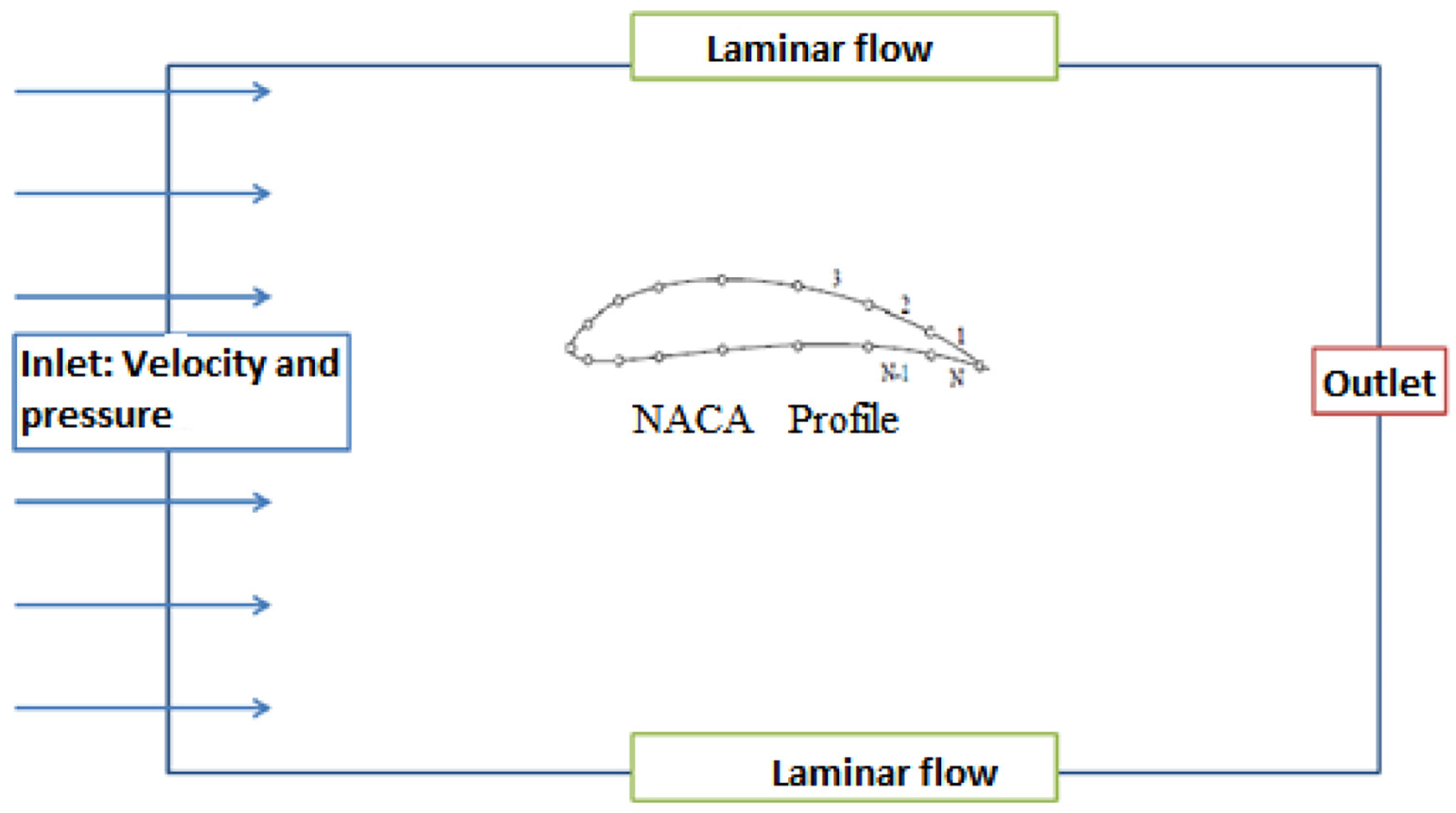
Representative scheme.

The boundary conditions, such as velocity and pressure, are imposed on a plate at a zero degree with velocity and pressure surrounding the airfoil of WT. The equations used are the Navier–Stokes equations in the Cartesian coordinates. In addition, these equations are solved by MSMs (RBF-FD).

Collocation MSM: RBFs

To illustrate the RBF method, let us consider the PDE, which is given by the following equation (Yensiri and Skulkhu, 2017)

Lu (x) = f (x) in x \in Ω

(1)

u (x) = g (x) on x \in \partial Ω

(2)

where L is the linear differential operator, N is the number of nodes, the boundary conditions are Dirichlet, Neumann, or mixed, and f and g are the functions.

Let $N$ be the number of nodes in a domain $Ω$ and $\partial Ω$ , the boundary of the domain. The RBF approximated solution u of equations (1) and (2) is

\hat{u} (x) = \sum_{j = 1}^{N} α_{j} ϕ_{j} (x)

(3)

where $ϕ_{j} (x) = ϕ (x - x_{j})$ is the RBF.

Replacing $u$ by $\hat{u}$ in equations (1) and (2), we have

L \hat{u} (x) = \sum_{j = 1}^{N} α_{j} L ϕ_{j} (x_{i}), 1 \leq i \leq N

(4)

\sum_{j = 1}^{N} α_{j} ϕ_{j} (x_{i}) = g (x_{i}), 1 \leq i \leq N + 1

(5)

Equations (4) and (5) can be written in the matrix form (Yensiri and Skulkhu, 2017) as equation (6)

[\begin{matrix} L ϕ \\ ϕ \end{matrix}] [α] = [\begin{matrix} f \\ g \end{matrix}]

(6)

Local MSM: RBF-FD method

For each node x_i, the function u, in the classical finite difference method in one dimension (1D), can be written by the following equation

\frac{d^{k} u (x_{i})}{d x^{k}} ≅ \sum_{j = 1}^{N} W_{i, j}^{(k)} u (x_{j})

(7)

The weight coefficients $W_{i, j}^{(k)}$ are computed by the polynomial interpolation. N is the numbers of nodes in the domain and u(x) is the function of node x_i.

The RBF for a set of points $x_{j}$ is given by (Javed et al., 2013)

u (x) = \sum_{j = 1}^{N} W_{j} ϕ (‖ x - x_{j} ‖) + β

(8)

where $ϕ (‖ x - x_{j} ‖)$ is the RBF, $j = 1, 2, \dots, N$ , $‖ \cdot ‖$ is the Euclidean norm between $x = (x_{i}, y_{i})$ and $x_{j} = (x_{j}, y_{j})$ ; and $W_{j}$ and $β$ are the expansion coefficients.

In the Lagrange form of RBF, equation (8) was written in the following form (Chandhini and Sanyasiraju, 2007)

u (x) = \sum_{j = 1}^{N} χ (‖ x - xj ‖) u (xj)

(9)

where $χ (‖ x - x_{j} ‖)$ satisfies

χ (‖ x - x_{j} ‖) = {\begin{matrix} 1, if k = j \\ 0, if \neq j \end{matrix} k = 1, 2, \dots, N

At node x₁, the differential operator L is given by the following form

Lu (x_{1}) = \sum_{j = 1}^{N} L χ (‖ x_{1} - x_{j} ‖) u (x_{j})

(10)

The weights of RBF-FD, expressed in equation (11), are obtained from equations (7) and (10)

W_{1, j}^{(L)} = L χ (‖ x_{1} - x_{j} ‖)

(11)

In the case of two dimension (2D), the weights W are solved by the system (Chinchapatnam et al., 2007; Javed et al., 2013) and can be written by the following equation

[\begin{matrix} ϕ & e \\ e^{T} & 0 \end{matrix}] [\begin{matrix} W \\ β \end{matrix}] = [\begin{matrix} L ϕ_{1} \\ 0 \end{matrix}]

(12)

where $ϕ (i, j) = ϕ (| | x_{1} - x_{j} | |),$ $1 \leq i, j \leq N$ , $1 \leq ei \leq N$ , L is the differential operator, and Lφ₁ is the column vector, $L ϕ_{1} = {[L ϕ ‖ x - x_{1} ‖ ‖ x - x_{2} ‖, \dots, x - x_{N}]}^{T}$ at node x₁ and β is a scalar parameter which imposes the condition

\sum_{j = 1}^{N} W_{1, j}^{L} = 0

(13)

WT aerodynamics modeling by MSM

The flow is assumed to be incompressible, irrotational, stationary, and frictionless. The equations of a conservation mass (the continuity equation) and momentum (Navier–Stokes equation) are written, respectively.

Continuity equation

\frac{\partial ρ}{\partial t} + div (ρ \vec{v}) = 0

(14)

where $\partial ρ / \partial t$ is the local derivative and $ρ$ is the density.

Equation of momentum

ρ (\frac{\partial \vec{v}}{\partial t}) + (\vec{v} \vec{grad}) \cdot \vec{v} = - \vec{grad} P + μ Δ \vec{v} + \vec{f}

(15)

where $v$ is the velocity, $p$ is the pressure, $f$ is the voluminal force, and $μ$ is the viscosity.

Considering the previous assumptions that the fluid is incompressible and stationary, the continuity equation is given by the following equation

div \vec{v} = 0

(16)

Equation (16) in 2D Cartesian coordinates is written by the following equation

\frac{\partial u}{\partial x} + \frac{\partial v}{\partial y} = 0

(17)

The irrotational flow is defined by

\vec{v} = \vec{grad} φ

(18)

Using equations (16) and (18), we obtain

Δ φ = 0

(19)

The vortex or vorticity vector $\vec{ω}$ is defined as the rotational velocity field

\vec{ω} = \vec{rot} \vec{v}

(20)

In 2D, the potential flow is given by equation (21)

ω = \frac{\partial v}{\partial x} - \frac{\partial u}{\partial y}

(21)

In terms of stream function, the velocity components of a 2D incompressible flow are given as

u = \frac{\partial ψ}{\partial y} = \frac{\partial φ}{\partial x}, v = - \frac{\partial ψ}{\partial x} = \frac{\partial φ}{\partial y}

(22)

In the case of 2D Cartesian coordinates, using equations (21) and (22), the potential function becomes

\frac{\partial^{2} ψ}{\partial x^{2}} + \frac{\partial^{2} ψ}{\partial y^{2}} = - ω

(23)

In the case of 2D Cartesian coordinates, stationary equation of momentum (15) is written as follows

{\begin{matrix} u \frac{\partial u}{\partial x} + v \frac{\partial u}{\partial y} = ν Δ u - \frac{1}{ρ} \frac{\partial P}{\partial x} \\ u \frac{\partial v}{\partial x} + v \frac{\partial v}{\partial y} = ν Δ v - \frac{1}{ρ} \frac{\partial P}{\partial y} \end{matrix}

(24)

Using the previous system, equation (24) is rewritten

u \frac{\partial ω}{\partial x} + v \frac{\partial ω}{\partial y} = \frac{1}{R_{e}} (\frac{\partial^{2} ω}{\partial x^{2}} + \frac{\partial^{2} ω}{\partial y^{2}})

(25)

The pressure can be obtained by solving an elliptic equation (taking the divergence of the Navier–Stokes equations). The pressure was calculated by the Poisson pressure-velocity equation

Δ P = 2 ρ (\frac{\partial u}{\partial x} \frac{\partial v}{\partial y} - \frac{\partial u}{\partial y} \frac{\partial v}{\partial x})

(26)

For the Navier–Stokes’s equations expressed in (23) and (25), the local MSM (RBF-FD) can be written as

{\begin{matrix} \sum_{j = 1}^{N} W_{i, j}^{(xx)} ψ_{j} + \sum_{j = 1}^{N} W_{i, j}^{(yy)} ψ_{j} = - ω_{i} \\ u_{i} \sum_{j = 1}^{N} W_{i, j}^{(x)} ω_{j} + v_{i} \sum_{j = 1}^{N} W_{i, j}^{(y)} ω_{j} = \frac{1}{R_{e}} (\sum_{j = 1}^{N} W_{i, j}^{(xx)} ω_{j} + \sum_{j = 1}^{N} W_{i, j}^{(yy)} ω_{j}) \end{matrix}

(27)

where: $N$ is the total number of nodes and boundaries in the support region for the node $x_{i}$ ; $W^{(x)}$ , $W^{(y)},$ $W^{(xx)}$ , and $W^{(yy)}$ are the weight coefficients of the RBF-FD method; u and v are the components of the velocity; and $R_{e}$ is the Reynolds number.

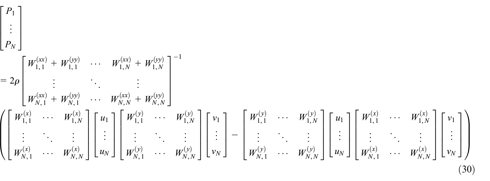
In local MSM (RBF-FD), the pressure equation can be written as equation (28)

\sum_{j = 1}^{N} W_{i, j}^{(xx)} P_{j} + \sum_{j = 1}^{N} W_{i, j}^{(yy)} P_{j} = 2 ρ (\sum_{j = 1}^{N} W_{i, j}^{(x)} u_{j} \sum_{j = 1}^{N} W_{i, j}^{(y)} v_{j} - \sum_{j = 1}^{N} W_{i, j}^{(y)} u_{j} \sum_{j = 1}^{N} W_{i, j}^{(x)} v_{j})

(28)

where N is the total number of nodes and boundaries in the support region for the node x_i and $W_{i, j}^{(x)}$ , $W_{i, j}^{(y)}$ , $W_{i, j}^{(xx)}$ and $W_{i, j}^{(yy)}$ are the weight coefficients of the RBF-FD method; u and v are the components of the velocity.

In matrix form, equation (28) can be rewritten as

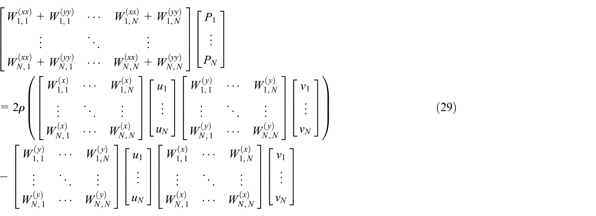
\begin{matrix} [\begin{matrix} W_{1, 1}^{(xx)} + W_{1, 1}^{(yy)} & \dots & W_{1, N}^{(xx)} + W_{1, N}^{(yy)} \\ ⋮ & ⋱ & ⋮ \\ W_{N, 1}^{(xx)} + W_{N, 1}^{(yy)} & \dots & W_{N, N}^{(xx)} + W_{N, N}^{(yy)} \end{matrix}] [\begin{matrix} P_{1} \\ ⋮ \\ P_{N} \end{matrix}] \\ = 2 ρ ([\begin{matrix} W_{1, 1}^{(x)} & \dots & W_{1, N}^{(x)} \\ ⋮ & ⋱ & ⋮ \\ W_{N, 1}^{(x)} & \dots & W_{N, N}^{(x)} \end{matrix}] [\begin{matrix} u_{1} \\ ⋮ \\ u_{N} \end{matrix}] [\begin{matrix} W_{1, 1}^{(y)} & \dots & W_{1, N}^{(y)} \\ ⋮ & ⋱ & ⋮ \\ W_{N, 1}^{(y)} & \dots & W_{N, N}^{(y)} \end{matrix}] [\begin{matrix} v_{1} \\ ⋮ \\ v_{N} \end{matrix}]) \\ - [\begin{matrix} W_{1, 1}^{(y)} & \dots & W_{1, N}^{(y)} \\ ⋮ & ⋱ & ⋮ \\ W_{N, 1}^{(y)} & \dots & W_{N, N}^{(y)} \end{matrix}] [\begin{matrix} u_{1} \\ ⋮ \\ u_{N} \end{matrix}] [\begin{matrix} W_{1, 1}^{(x)} & \dots & W_{1, N}^{(x)} \\ ⋮ & ⋱ & ⋮ \\ W_{N, 1}^{(x)} & \dots & W_{N, N}^{(x)} \end{matrix}] [\begin{matrix} v_{1} \\ ⋮ \\ v_{N} \end{matrix}] \end{matrix}

(29)

Pressure deduction can be presented as equation (30)

\begin{matrix} [\begin{matrix} P_{1} \\ ⋮ \\ P_{N} \end{matrix}] \\ = 2 ρ {[\begin{matrix} W_{1, 1}^{(xx)} + W_{1, 1}^{(yy)} & \dots & W_{1, N}^{(xx)} + W_{1, N}^{(yy)} \\ ⋮ & ⋱ & ⋮ \\ W_{N, 1}^{(xx)} + W_{N, 1}^{(yy)} & \dots & W_{N, N}^{(xx)} + W_{N, N}^{(yy)} \end{matrix}]}^{- 1} \\ ([\begin{matrix} W_{1, 1}^{(x)} & \dots & W_{1, N}^{(x)} \\ ⋮ & ⋱ & ⋮ \\ W_{N, 1}^{(x)} & \dots & W_{N, N}^{(x)} \end{matrix}] [\begin{matrix} u_{1} \\ ⋮ \\ u_{N} \end{matrix}] [\begin{matrix} W_{1, 1}^{(y)} & \dots & W_{1, N}^{(y)} \\ ⋮ & ⋱ & ⋮ \\ W_{N, 1}^{(y)} & \dots & W_{N, N}^{(y)} \end{matrix}] [\begin{matrix} v_{1} \\ ⋮ \\ v_{N} \end{matrix}] - [\begin{matrix} W_{1, 1}^{(y)} & \dots & W_{1, N}^{(y)} \\ ⋮ & ⋱ & ⋮ \\ W_{N, 1}^{(y)} & \dots & W_{N, N}^{(y)} \end{matrix}] [\begin{matrix} u_{1} \\ ⋮ \\ u_{N} \end{matrix}] [\begin{matrix} W_{1, 1}^{(x)} & \dots & W_{1, N}^{(x)} \\ ⋮ & ⋱ & ⋮ \\ W_{N, 1}^{(x)} & \dots & W_{N, N}^{(x)} \end{matrix}] [\begin{matrix} v_{1} \\ ⋮ \\ v_{N} \end{matrix}]) \end{matrix}

(30)

WT NACA airfoil profile modeling by MSM

For the sake of illustration only and due to benchmark comparison possibilities, a NACA profile has been selected for the shape of the WT aerofile.

Definition

The NACA airfoils are Airfoil shapes for aircraft wings developed by the NACA. The shape of the NACA airfoils is described, using a series of digits following the term NACA.

The typical NACA is illustrated in Figure 2 by a few parameters, such as maximum thickness, maximum camber, position of maximum thickness, position of maximum camber, along with leading edge, trailing edge, chord length, and leading edge radius.

Figure 2.

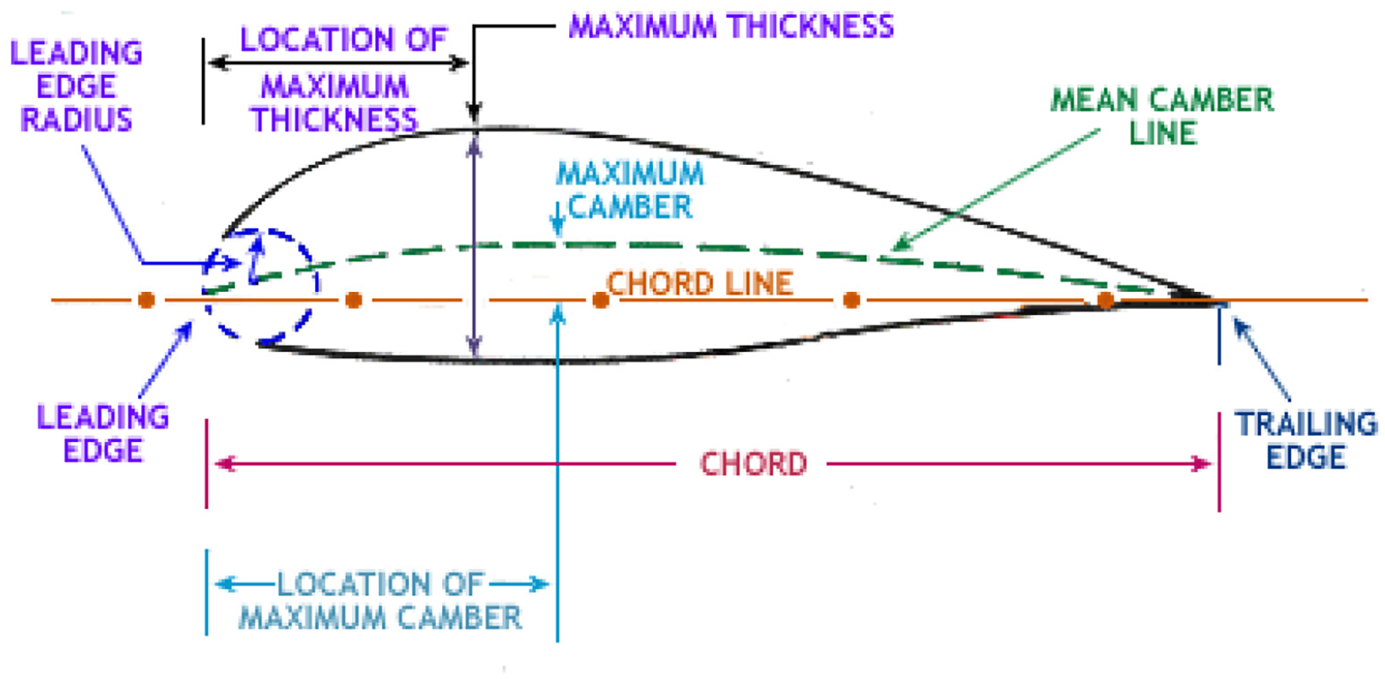
Typical NACA airfoil showing associated terminologies.

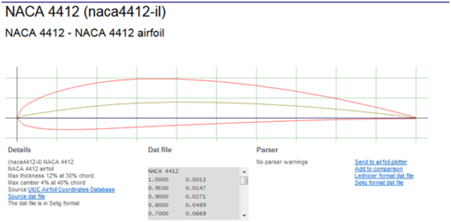
The WT blade NACA 4412 airfoil, as shown in Figure 3, which is asymmetric biconvex airfoils, is also brought at zero incidences and is very stable.

Figure 3.

NACA 4412 airfoil.

The digit number and characteristics of the blade turbine NACA 4412 profile airfoil represent 4%, which is the maximum camber in percentage of chord, 40% represent the location of maximum camber in percentage of chord, and 12% represent the maximum thickness in percentage of chord (Genç et al., 2019).

Boundary conditions

The conditions applied to the boundaries are determined according to four zones. These boundary condition zones are known as inlet, outlet, wall, and NACA. At the inlet, velocity is constant and is specified as 10 m/s. The wall motion is stationary, and in the shear condition: no slip is observed. Concerning the outlet, the default value for pressure of $0$ Pascal and the zero velocity gradient condition are used. The condition around a NACA airfoil is fixed and the velocity is zero.

WT NACA airfoil profile modeling by MSM

Meshing using FEM

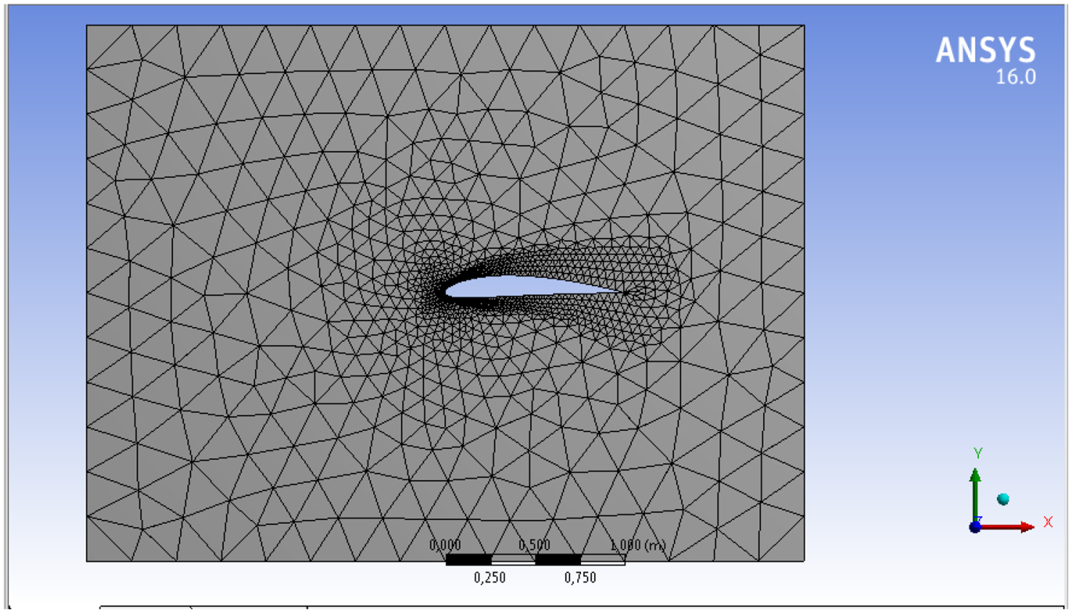
In 2D Cartesian coordinates, refinement is a necessary phase to determine the optimum mesh. Thus, generally, the mesh structure is very tight in the vicinity of the airfoil and even in the leading edge and trailing edge recirculation zones in order to properly simulate the flow. Triangular mesh has several advantages, such as (1) it can be generated on a complex geometry while keeping good quality elements and (2) the generation algorithms of this type of mesh (tri/tetra) are automated. The sizing around the blade after refinement and the triangular mesh are illustrated in Figure 4.

Figure 4.

Mesh blade wind turbine airfoil of HAWT by Ansys in two dimension.

For this 2D configuration, the number of nodes is 1730 and the number of elements is 3232 (triangular).

Meshing using local MSM: RBF-FD method

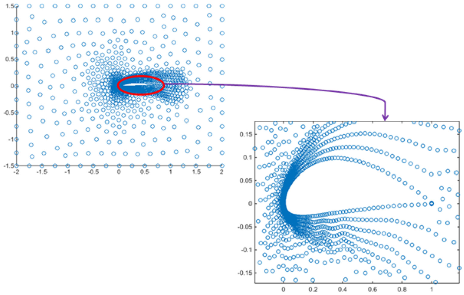
To obtain the number of nodes in mesh, the Nlist commands to a command file, and this gives the positional and connectivity data that MATLAB needs. The importation of the mesh of nodes was done using an automatic generator of Ansys and these nodes were exploited to extract the nodes around the NACA profile 4412 to MATLAB environment.

The 1730 nodes are shown in Figure 5:

Figure 5.

Meshless method for blade airfoil of WT.

Numerical results

Consider the laminar flow around a NACA airfoil profile of a horizontal WT, the chord is $c = 1 m$ . The number of nodes (ox) is $nx = 100$ and the number of nodes (oy) is $ny = 100$ . The fluid used is the air which is assumed to be incompressible and stationary with the following characteristics

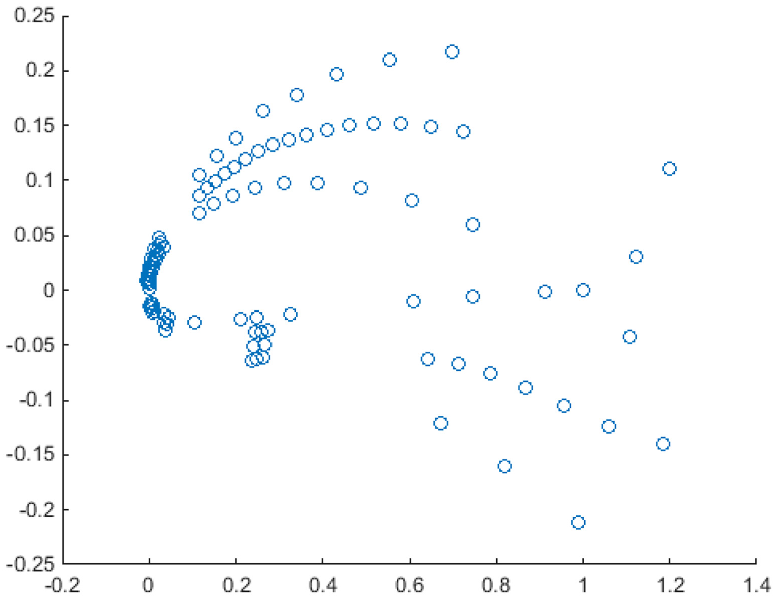
Initial velocity: $U = 10 m / s,$ dynamic viscosity of the fluid: $μ = 0.06 kg / ms$ , and density: $ρ = 1.225 kg / m^{3}$ .

In the MSM, the nodes around the blade of a WT airfoil where $N = 100$ with 2D coordinates along the $x$ and $y$ axes are shown in Figure 6.

Figure 6.

Wind turbine blade NACA 4412 airfoil (N = 100).

The velocity around the airfoil of the WT, using an FEM, is shown in Figure 7.

Figure 7.

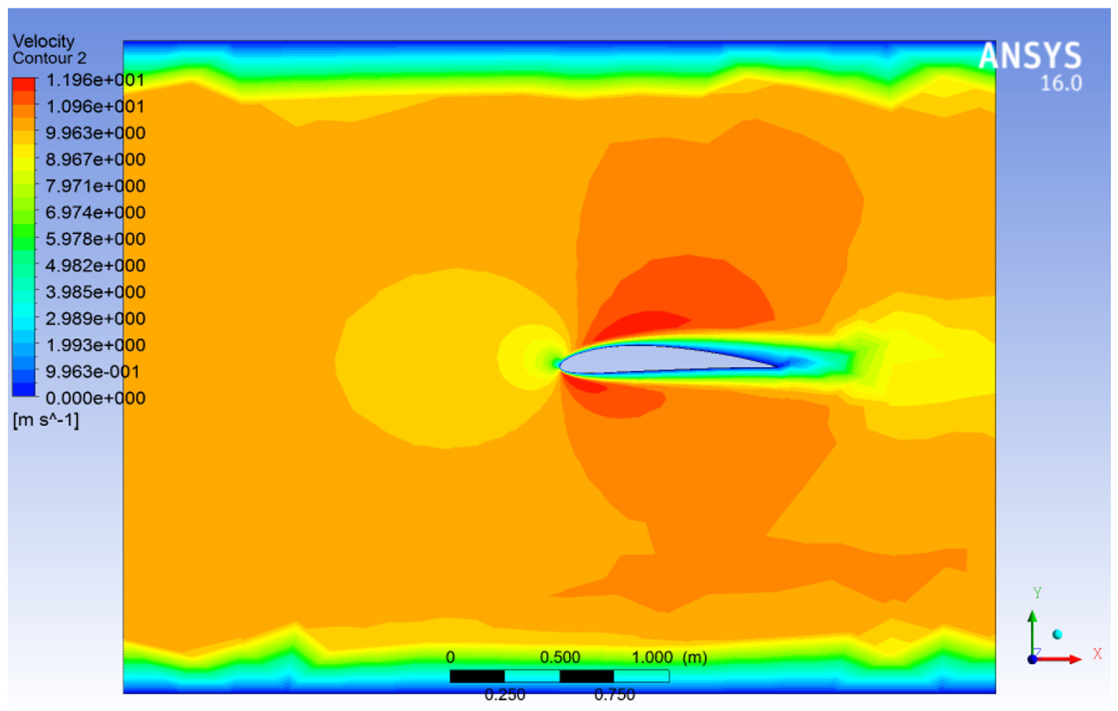
Velocity by FEM: Ansys.

The velocity of the local MSM is shown in Figure 8: Figures 7 and 8 show the contours as well as the velocity field around the airfoil of a WT by MSM and FEM, respectively. At the inlet, the speed is uniform and equal to 10 m/s, as a condition of the initial limits. We can observe an acceleration of the speed between the wall and the blade airfoil of the WT; this is due to the decrease in the section of the passage of the fluid. In this regard, there is a conversion of the energy of the fluid. Afterward, at the downstream of the airfoil profile, according to the regime and the Reynolds number, a particular flow appears, resulting in a new point of delimitation of the fluid each time. At the leading edge, it increases between 6 and 8, and in the trailing edge, it is zero.

Figure 8.

Velocity by meshless method N = 100.

The local MSM gives good results without any error and with precision in the flow of the fluid in the laminar and stationary cases and around the NACA 4412 airfoil profile as compared to the FEM, which gives errors in the fluid and around the airfoil in an interval of 0–12 m/s. The local MSM gives a reduction in the number of nodes as compared to FEMs for 100 nodes.

The pressure around the blade of WT by FEM is shown in Figure 9.

Figure 9.

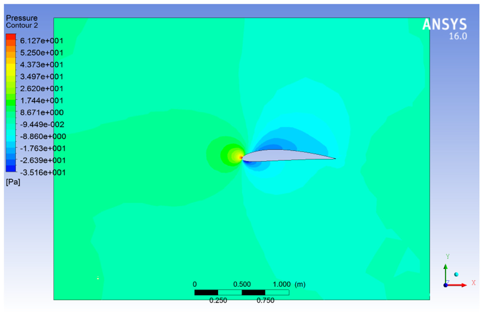
Pressure by FEM: Ansys

The pressure of local MSM is presented in Figure 10.

Figure 10.

Pressure by meshless method N = 100.

In the interval −30 Pa and+60 Pa, for the distribution of pressure, the pressure reaches a maximum in the leading edge which can reach up to 60 Pa and a minimum on both surfaces (extrados and intrados) of −30 Pa, as shown in Figure 10. Applying the Bernoulli relation for incompressible fluids and when the velocity is high, the minimum pressure (low pressure) is said to be in depression, whereas when the velocity is minimal, the velocity is low and the pressure is at overpressure (high pressure). It reaches its maximum.

Discussion

In our results, the NACA 4412 airfoil profile by local method meshless: RBF-FD was presented. We were able to solve by the use of Navier–Stokes equations in the laminar, incompressible, and stationary case around the NACA profile. The local RBF-FD method has the following advantages: feasibility and calculation. Also, this method gives more precision for complex geometries aerodynamic such as the NACA 4412 profile which consists of optimizing and improving the parameters such as nodes. These nodes are introduced for the numerical solution in the Navier–Stokes equation. The importance of precision is very useful in the local RBF-FD method because the matrix system is well conditioned and can be reversible for the number of nodes tested.

The NACA 4412 profile in 2D for WTs is effective in reducing errors around the blade boundaries. Therefore, the RBF-FD has a very interesting and important role at the level of the NACA 4412 airfoil in terms of precision, regarding the calculation. It is also easy to represent in comparison to the FEM obtained by Ansys, which gives the errors for the velocity and pressure.

Conclusion

In this work, we presented the novel local MSM (RBF-FD) in aerodynamics of the HAWT. The principal purpose of this method is to extract the nodes for complex geometry such as NACA 4412 airfoil profile WT. These nodes have an important role: First, they have good precision.

Second, they obtain an optimal geometry for location problems. Third, they are easy to represent complex domains, such as the NACA profile. These nodes have been used in the Navier–Stokes equation in the hypotheses laminar, stationary, and incompressible flow by RBF-FD method in 2D.

Likewise, in this study, we showed the importance of local MSM in aerodynamic and minimized the computation duration.

In the numerical results, we tested 100 nodes of velocity and pressure in close agreement with the FEM. Moreover, the results of the local MSM and FEM were comparable and gave behavior of the flow around the profile. Therefore, the use is to regularize and increase the parameter design of thee NACA profile.

In the future, the model will be used for the entire blade WT in three dimension (3D) by the local MSM: RBF-FD.

Footnotes

Declaration of conflicting interests

The author(s) declared no potential conflicts of interest with respect to the research, authorship, and/or publication of this article.

Funding

The author(s) received no financial support for the research, authorship, and/or publication of this article.

ORCID iD

Asmae Mnebhi-Loudyi

References

Ackermann

(2005) Historical development and current status of wind power-wind power in power systems. Book. Available at: https://onlinelibrary-wiley-com-443.web.bisu.edu.cn/doi/abs/10.1002/9781119941842.ch3

Ahmad

Siraj-ul-Islam (2018) Meshless analysis of parabolic interface problems. Engineering Analysis with Boundary Elements 94: 134–152.

Beri

Yao

(2011) Effect of camber airfoil on self starting of vertical axis wind turbine. Journal of Environmental Science and Technology 4(3): 302–312.

Chandhini

Sanyasiraju

YVSS

(2007) Local RBF-FD solutions for steady convection-diffusion problems. International Journal for Numerical Methods in Engineering 72(3): 352–378.

Chinchapatnam

Djidjeli

Nair

(2007) Radial basis function meshless method for the steady incompressible Navier-Stokes equations. International Journal of Computer Mathematics 84(10): 1509–1521.

Chinchapatnam

Djidjeli

Nair

, et al. (2009) A compact RBF-FD based meshless method for the incompressible Navier-Stokes equations. Proceedings of the Institution of Mechanical Engineers, Part M: Journal of Engineering for the Maritime Environment 223(3): 275–290.

El Khchine

Sriti

Ouariaglim

(2015) Simulation Des Performances Aerodynamiques d’une eolienne a axe Horizontal. 22ème Congrès Français de Mécanique, Lyon, 24–28 Août, pp. 5.

Genç

Koca

Açikel

(2019) Investigation of pre-stall flow control on wind turbine blade airfoil using roughness element. Energy 176: 320–334.

Govind

(2017) Increasing the operational capability of a horizontal axis wind turbine by its integration with a vertical axis wind turbine. Applied Energy 199: 479–494.

10.

Guerri

Hamdouni

Sakout

(2008a) Fluid structure interaction of wind turbine airfoils. Wind Engineering 32(6): 539–557.

11.

Guerri

Hamdouni

Sakout

(2008b) Numerical simulation of the flow around oscillating wind turbine airfoils, part 1: Forced oscillating airfoil. The International Journal of Multiphysics 2(4): 367–385.

12.

Hsu

(2011) Dynamic analysis of wind turbine blades using radial basis functions. Advances in Acoustics and Vibration 2011: 973591.

13.

Javed

Djidjeli

Xing

, et al. (2013) A hybrid mesh free local RBF-Cartesian FD scheme for incompressible flow around solid bodies. International Journal of Mathematical, Computational, Physical, Electrical and Computer Engineering 7(10): 61–70.

14.

Kansa

(1990) Multiquadrics—A scattered data approximation scheme with applications to computational fluid-dynamics. 2. Solutions to parabolic, hyperbolic and elliptic partial-differential equations. Computers & Mathematics with Applications 19(8–9): 147–161.

15.

Mathew

(2006) Wind Energy: Fundamentals, Resource Analysis and Economics. Berlin; Heidelberg: Springer. Available at: https://www.springer.com/gp/book/9783540309055

16.

Shu

Ding

Yeo

(2003) Local radial basis function-based differential quadrature method and its application to solve two-dimensional incompressible Navier-Stokes equations. Computer Methods in Applied Mechanics and Engineering 192(7–8): 941–954.

17.

Stevens

Power

Lees

, et al. (2009) The use of PDE centres in the local RBF Hermitian method for 3D convective-diffusion problems. Journal of Computational Physics 228: 4606–4624.

18.

Lei

Zhou

, et al. (2019) Aerodynamic noise assessment for a vertical axis wind turbine using improved delayed detached eddy simulation. Renewable Energy 141: 559–569.

19.

(2019) A radial basis function (RBF)−finite difference (FD) method for the backward heat conduction problem. Applied Mathematics and Computation 354: 232–247.

20.

Tabbakh

Seaid

Ellaia

, et al. (2019) A local radial basis function projection method for incompressible flows in water eutrophication. Engineering Analysis with Boundary Elements 106: 528–540.

21.

Tahir

Elgabaili

Rajab

, et al. (2019) Optimization of small wind turbine blades using improved blade element momentum theory. Wind Engineering 43(3): 299–310.

22.

Tolstykh

Shirobokov

(2003) On using radial basis functions in a finite difference mode with applications to elasticity problems. Computational Mechanics 33(1): 68–79.

23.

Wright

Fornberg

(2006) Scattered node compact finite difference-type formulas generated from radial basis functions. Journal of Computational Physics 212(1): 99–123.

24.

Lang

Zargari

, et al. (2011) Power conversion and control of wind energy systems. Book. Available at: https://onlinelibrary-wiley-com-443.web.bisu.edu.cn/doi/book/10.1002/9781118029008

25.

Sankar

(2000) Computational study of horizontal axis wind turbines. Journal of Solar Energy Engineering 122(1): 35–39.

26.

Yensiri

Skulkhu

(2017) An investigation of radial basis function-finite difference (RBF-FD) method for numerical solution of elliptic partial differential equations. Mathematics 5(4): 54.

27.

Zhou

Zhang

, et al. (2009) Numerical investigation of violent wave impact on offshore wind energy structures using MLPG_R method. In: Proceedings of the nineteenth international offshore and polar engineering conference, Osaka, Japan, 21–26 June, pp. 1351–1356. Mountain View, CA: International Society of Offshore and Polar Engineers.