Computational fluid dynamics study of Savonius rotors using OpenFOAM

Abstract

In this work, two-dimensional models of Savonius rotors are simulated using OpenFOAM^® in order to predict the aerodynamic performance of small-scale vertical-axis wind turbines. The results are reported analyzing the aerodynamic performance and forces acting on the rotors. Power coefficient, $(C_{P})$ , is compared with experimental data for each operation point, and for three different geometries. Simulations with first- and second-order discretization schemes are carried out and compared, both quantitative and qualitative. Since usual grid dimensions result not to be suitable for simulations of Savonius rotors, an analysis of different domains is performed and compared. Finally, a set up for computational fluid dynamics simulation of two-dimensional Savonius rotors is proposed. The fluid–rotor interaction is analyzed and the vortex shedding is correlated with $C_{P}$ values and wake description.

Keywords

Computational fluid dynamics vertical-axis wind turbine Savonius OpenFOAM wind engineering

Introduction

While the wind energy technology is mature at big scale, this is not the case for smaller scales, where the technology has not been consolidated. Different models can be considered depending on the environment, and different designs to fit different applications. The wind profile in urban areas is characterized by lower mean wind speed and larger fluctuations in directions and magnitude. The horizontal-axis wind turbines (HAWTs) are not adequate for operation in urban areas, since they demand an orientation system and the blades are prone to damage in high turbulence conditions. Meanwhile, vertical-axis wind turbines (VAWT) are less dependent on wind direction fluctuations, and different designs can be adapted, considering the wind flow characteristics and mechanical solicitations, being therefore, more suitable for turbulent conditions. The classic VAWT types are Darrieus and Savonius turbines. Despite having lower efficiency than Darrieus rotors, Savonius design present several advantages such as, self-starting capability, low cut in wind speed, simplicity, and low construction costs. However, their aerodynamic performance is not easy to predict or analyze. As it expressed by Modi and Fernando (1993), the theoretical prediction of Savonius rotor performance is difficult by the complexity of the air around it and the mutual interference of the buckets. One model—perhaps the only one—noticed by Paraschivoiu (2002) is a mathematical model proposed by Chauvin et al. (1983), which enables computing the power of two-bucket Savonius rotor without any gap between the buckets; however, this gap is an essential parameter in this geometry. Therefore, there are mainly only two ways to investigate the aerodynamic performance of Savonius rotors: computational fluid dynamic (CFD) models or experimental tests.

Vignolo et al. (2015) studies the economic feasibility of VAWT for on-grid residential applications in Uruguay. In 2015, considering the residential electrical energy price and the commercial VAWTs prices, the installation of these turbines was not a good option from an economical point of view. A further work, González and Cataldo (2019), shows that for Uruguay, the market is starting to be attractive for micro wind applications, since the prices of the energy tends to rise while the prices of VAWTs tends the opposite and the payback is close to an acceptable period of time. Consolidating an useful tool for the design of this type of turbines could be a step forward into the implementation of micro wind technology in urban environments for distributed generation, in the search for prototypes that fit the technological and economic demands.

Some two-dimensional (2D) numerical studies of Savonius rotors are found in the literature, such as Akwa et al. (2012), Alom and Saha (2018), Kacprzak et al. (2013), and Shaheen et al. (2015). Rezaeiha et al. (2018) noted that for Darrieus rotors, there is a lack of extensive parametric studies investigating the impacts of different computational parameters in the accuracy of the results, and for Savonius rotors, this is even worse. In Dobrev and Massouh’s (2011) study, a discussion about the differences between using Reynolds-averaged Navier–Stokes (RANS) and detached eddy simulation (DES) models for CFD simulations of Savonius rotors is made, indicating that for 2D simulations RANS model with k-w shear stress transport (SST) turbulence model is the most suitable configuration. Nasef et al. (2013) also studied the performance sensitivity of a two-bucket Savonius using RANS model to the turbulence model and concluded that $k - w$ SST model is suitable for simulating the flow pattern around the Savonius rotor than other models for both stationary and rotating cases.

In this work, an extensive parametric study of the influence of gird, domain size, and discretization schemes on the simulation of Savonius VAWTs is carried out.

Savonius wind turbine

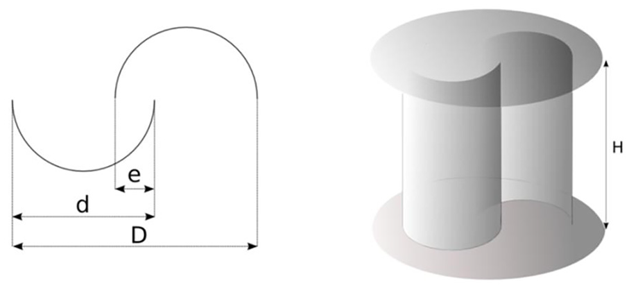
In urban areas, where the wind flow is highly turbulent and affected by obstacles, VAWT rotors are more suitable than HAWT. They are more robust for these conditions and are not as sensible as HAWT rotors to changes in wind direction and turbulence. The wind data measurements within a city show lower mean velocities than in open-field terrains, and therefore, Savonius rotors may be more adequate, showing the best power performances at low wind velocities. In these types of rotors, the working principle is based on the difference of the drag force between convex and concave parts of the rotor blades when they rotate around a vertical shaft. The scheme in Figure 1 shows the dimensions of the rotor. The buckets overlap is a crucial parameter in its performance and it is characterized by a dimensionless parameter, overlap ratio $(OR)$

OR = \frac{e}{d}

(1)

Figure 1.

Savonius scheme.

To characterize the wind turbine performances, the power coefficient $C_{P}$ , presented in equation (2), is used. It represents the fraction of the extracted power by the turbine from the total available in free stream of air flow at undisturbed velocity $V_{\infty}$ , that runs through the projected area of the rotor

C_{P} = \frac{P}{P_{available}} = \frac{M ω}{1 / 2 ρ (DH) v_{\infty}^{3}}

(2)

In equation (2), $P$ and $M$ are the rotor power and moment, $ρ$ is the air density, $D$ and $H$ are the rotor diameter and height, giving the swept area, and $ω$ is the rotational speed. The parameter is analyzed through its behavior with the tip speed ratio, $λ$ , computed as the ratio between peripheral velocity and upstream velocity

λ = \frac{R ω}{v_{\infty}}

(3)

where $R$ is the radius of the rotor $(R = D / 2)$ .

Benchmark

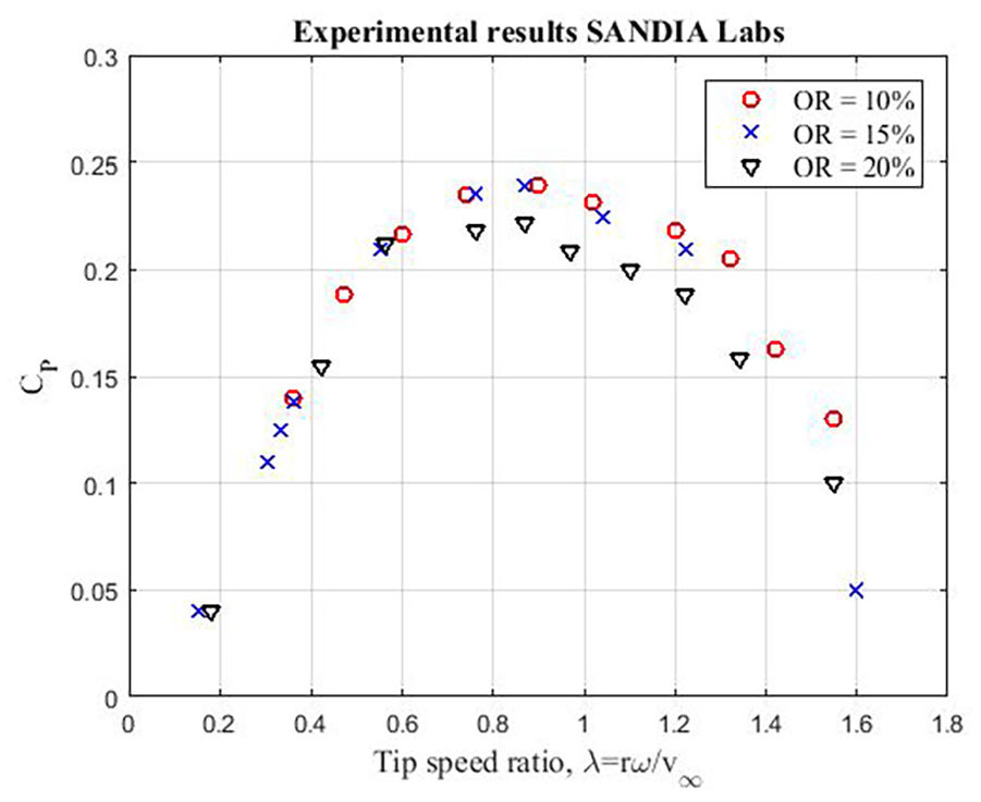
Blackwell et al. (1977) shows experimental tests performed in the wind tunnel for Savonius rotors. The results obtained in those experiments are used as a benchmark of the aerodynamic performance of such rotors. Figure 2 shows the power coefficients obtained in the reference work for 1 m, two-buckets Savonius rotors with three different ORs at $Re / m$ of $4.32 \times 10^{5}$ .

Figure 2.

Experimental results SANDIA (Blackwell et al., 1977).

The rotors tested have no twist angle and have end plates on both sides that limit the three-dimensional (3D) flow behavior around the model. The experimental results show that the best performance coefficients are obtained for $OR$ values between 0.10 and 0.15. Many works studied how the OR influences the performances rotors (Akwa et al., 2012; El-Askary et al., 2015; Gupta et al., 2008; Jian et al., 2012; Mojola, 1985), and, even that there is not a complete agreement on the optimal value for $OR$ , the range is between 0.15 and 0.25. In this study, three values of OR are taken into account, and then $OR = 0.15$ is considered to perform further analysis and performance sensitivity to different configuration settings.

Computational settings

Numerical models and operation parameters

Within OpenFOAM software, the incompressible unsteady Reynolds-averaged Navier–Stokes (URANS) package is used to perform the simulations. The pressure–velocity coupling is solved with PIMPLE method (combination of SIMPLE and PISO solvers). This is the selected solver, adequate for transient, incompressible, and turbulent flow of Newtonian fluids on moving meshes.

Previous works like Ferrari et al. (2017), Marmutova (2016), Nasef et al. (2013), and Shaheen et al. (2015), show that URANS with $k - w$ SST models are appropriate for simulating turbulence in 2D Savonius rotors models with a reasonable computational cost. Despite this, it is worth to notice that some simulations took up to 2 weeks of running time in a cluster to simulate 4 s of operation. The turbulence model used is the $k - w$ SST, for which studies like that of Al-Faruk and Sharifian (2017) show that it is suitable for simulating the flow pattern around the Savonius rotor rather than other models for both stationary and rotating cases.

Simulations of 2D Savonius rotor in OpenFOAM with the $k - w$ SST turbulence model are analyzed and compared to the experimental data available. This is done comparing the coefficient of power $(C_{P})$ for each point of operation.

Computing the forces on the surfaces of the buckets in OpenFOAM and using the rotation speed allows to calculate the power exchange with the flow, and therefore the $C_{P}$ . For this methodology is crucial to have a good description of the boundary layer developed on the rotor surfaces. The same free-stream velocity is fixed as in the experimental study which used a benchmark value of 7 m/s, and a turbulence intensity of $1 %$ is considered. Different operation points are evaluated using the same free-stream velocity and changing the rotational speed $(w)$ , and therefore, the tip speed ratio $λ$ .

Numerical schemes

The performance sensitivity due to the numerical discretization is analyzed. First- and second-order derivatives were considered, both for time and for space gradients.

CFD schemes 1

In this first configuration, Euler scheme is used for time discretization. As it is presented in Moukalled et al. (2016), the transient first-order implicit Euler scheme is obtained using a first-order interpolation profile, resulting in

\frac{{(ρ φ)}^{t} - {(ρ φ)}^{(t - δ t)}}{δ t} V_{C} + L (φ^{t}) = 0

(4)

where $V_{C}$ is the volume of the discretization element, and $L (φ^{t})$ is a spatial discretization operator that includes all non-transient terms. This implicit discretization is stable, but could miss transient phenomena if the time step is not small enough. The solution it yields is really a stationary solution for large time steps. The divergence schemes for velocity, $k$ and $ω$ are also first-order, named as Gauss Upwind. In OpenFOAM, the schemes are all based on Gauss integration, being interpolated to the cell faces, Upwind for this first case. The mathematical analysis of this discretization leads to an equation with an added component of diffusion, which is called truncation error. This error, also known as stream wise diffusion, reduces the accuracy of the solution by altering the magnitude of the diffusion coefficient and consequently the equation to be solved. On the contrary, this additional stream-wise numerical diffusion is desirable as it stabilizes the solution by keeping it bounded and physically correct.

CFD schemes 2

In this second case studied, the time discretization used is second-order and implicit scheme, called Backward in OpenFOAM. The mathematical analysis for this second-order interpolation profile, results in the following expression (Moukalled et al., 2016)

\frac{3 (ρ φ)^{t - 4} {(ρ φ)}^{(t - δ t)} + {(ρ φ)}^{(t - 2 δ t)}}{2 δ t} V_{C} + L (φ^{t}) = 0

(5)

Divergences are also second order; for the velocity bounded Gauss linearUpwind is used and bounded Gauss Upwind for $k$ and $ω$ .

Turbulence model

The SST $k$ - $ω$ turbulence model is used in this study. Menter (1993) developed this two-equation eddy-viscosity model which has become very popular. The SST uses $k$ - $ω$ formulation in the inner parts of the boundary layer. The SST switches to a $k$ - $ε$ behavior in the free stream and thereby avoids the common $k$ - $ω$ problem, when the model is too sensitive to the inlet free-stream turbulence properties. The SST $k$ - $ω$ model presents a good behavior in adverse pressure gradients and separating flow, which is the case of flow around VAWTs. The turbulence model needs to determine the turbulent kinetic energy $k$ (equation (3)) and the specific turbulent dissipation rate $ω$ (equation (4))

k = \frac{3}{2} (v_{\infty} . I)^{2}

(6)

ω = \frac{C_{m} . k^{0.5}}{L}

(7)

where $I$ is the turbulence intensity, $C_{m}$ is the turbulence model constant that takes a value of 0.09, and $L$ is the reference length scale. In a wind tunnel, the turbulence intensity in the inflow is expected to be close to $1 %$ ; therefore, this value was assumed to calculate $k$ and $ω$ . Turbulence intensity in the inflow is a parameter that has a major relevance for urban environment, but this study pretends to adjust the numerical CFD as a prediction tool, using the experimental results in a wind tunnel as reference values.

Domain and grid description

The geometry of a Savonius and the computational domain of the numerical modeling are developed using Pointwise^®. The rotor geometry applied is a 2D slide with the same dimensions as the rotors essayed by SANDIA Laboratories (Blackwell et al., 1977).

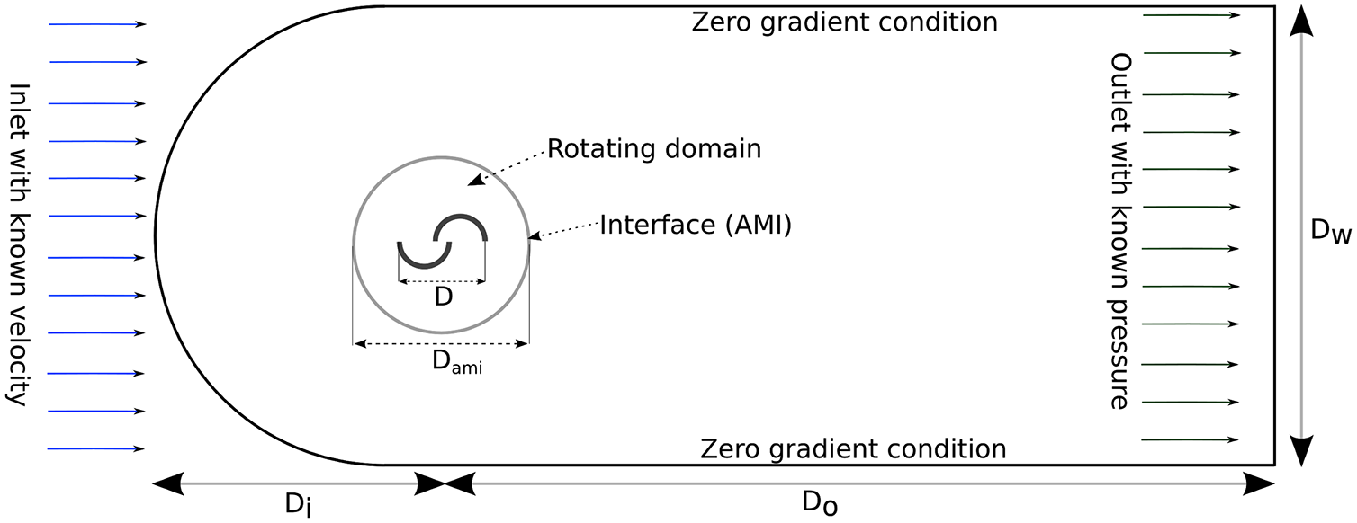
Figure 3 shows a scheme of the whole domain, as well as the boundary conditions used.

Figure 3.

Description of the domain.

The mesh is conformed by two zones: the inner circular zone that includes the rotor geometry and rotates with an imposed angular velocity, and the outer zone that completes the domain and is fixed. The cells in the interface between the inner and the outer regions are uniform. The inner and outer mesh are coupled using the OpenFOAM function arbitrary mesh interface (AMI), which enables simulation across disconnected, adjacent, mesh domains. The impact of rotating domain diameter $(D_{AMI})$ was found to be negligible, and it is in concordance with the results obtained by Rezaeiha et al. (2018). Meanwhile, the size of the domain has a sensitive impact on the performance coefficient as it is presented in the next sections.

It is essential to have a good description of the boundary layer over the rotor to determine accurately the efforts, and therefore, the power coefficient. The dimensionless parameter $y^{+}$ , used to define the distance between the cell and the wall, is imposed to be no greater than the unit. This is a very strong condition, that leads to a very fine mesh close to the rotor but necessary to describe accurately the boundary layer avoiding the use of wall functions. The size of the first cell of the mesh next to the wall is $Δ s$ . It can be computed for given values of $y^{+}$ and $Re$ . This is done based on flat-plate boundary layer theory exposed by White (2003)

Re = \frac{U_{\infty} L}{ν}

(8)

Following this approach, we obtain the size of cells next to the rotor’s wall for $y^{+} = 1$ condition

Δ s = \frac{y^{+} ν}{u^{*}}

(9)

The maximum Reynolds number condition was used for the previous calculations, and therefore, conform a grid adequate for all the cases simulated. Several inner meshes, with different numbers of cells, were run to study its independence. Grids were compared maintaining the overall shape, but reducing every cell by a $\sqrt{2}$ factor, seeking the grid convergence. The refined zone next to the rotor is a structured grid with $Δ s = 2.1 \times 1 0^{- 5} m$ and a growth rate of 1.1 up to a distance of the rotor walls. From there on, an unstructured zone links with a circular external zone that completes the inner rotating zone. The inner mesh is composed of 315,000 cells. Despite that, with a coarse grid, the results obtained were the same, and this mesh assures that for different operation points and different simulation parameters, the inner mesh will play no role in the results.

The outer mesh varies in its cells numbers since different domain sizes were considered as it is shown in the next sections.

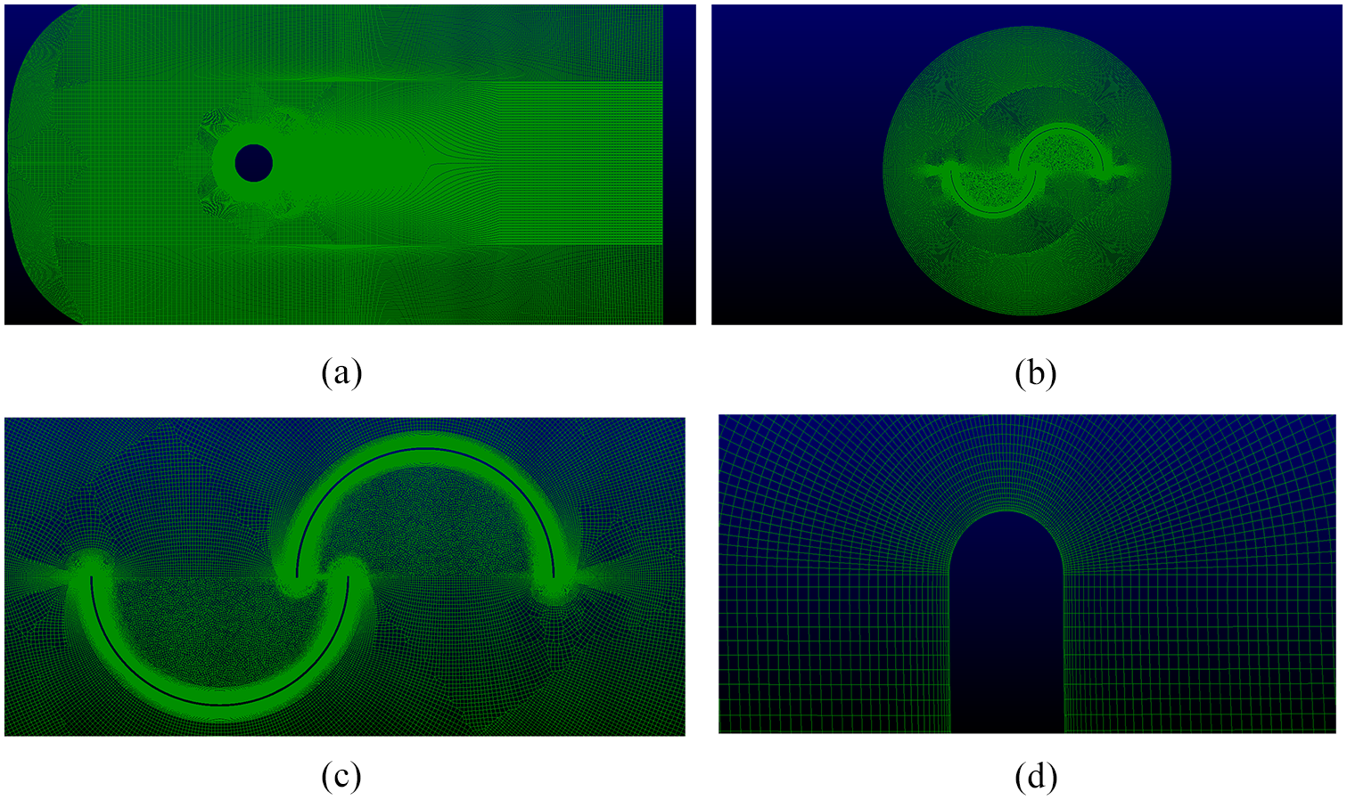
Figure 4 shows some details of the final inner and outer mesh. The outer mesh, which defines the domain size, can be seen in Figure 4(a), where there is a circular empty space instead of the inner mesh.

Figure 4.

Different views of the mesh for the Savonius rotor: (a) outer fixed mesh, (b) inner rotating mesh, (c) rotor mesh, and(d) zoom in rotor walls (rotor tip).

Results and verification

For each configuration essay in the experimental reference work, a case in OpenFOAM was created. The inlet velocity is imposed as well as the rotational speed, then $C_{P}$ is computed and compared with the experimental results. For CFD simulations, the resultant torque is calculated for each time step, and then the mean power and the $C_{P}$ is obtained.

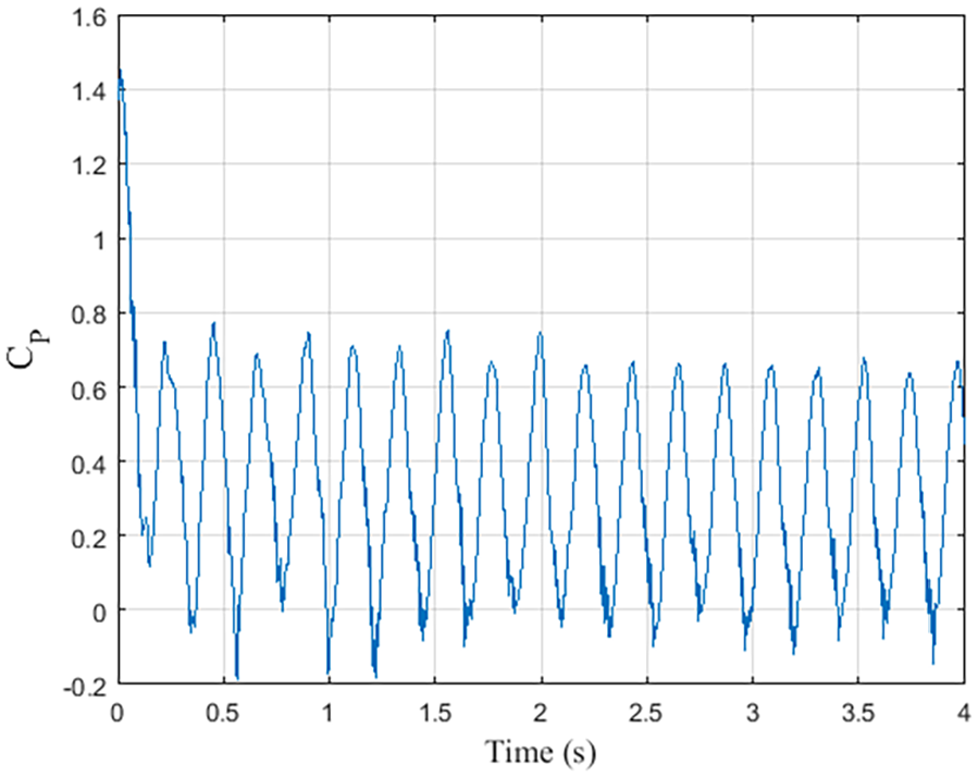
The interaction between rotor and flow take some time to reach stability. Despite the time to stabilize varies for each case, it is observed that 1 s is enough for the power coefficient to establish around a constant mean value in all the cases. Figure 5 shows the Cp evolution in time for a given case.

Figure 5.

Evolution of power coefficient over time. $OR = % 15$ , $λ = 1.2$ .

This mean value is obtained for each $OR$ and $λ$ simulated and compared with the experimental data.

Since the CFD simulations are based on URANS modelation, there are some uneven fluctuations that do not vanish over time. This is as expected, considering that the phenomena is highly turbulent and do not behave as a perfect cycle.

Numerical sensitivity

First-order schemes

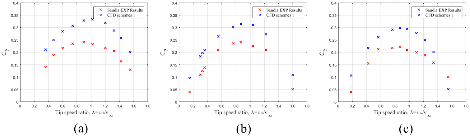
The first study is performed using mainly first-order schemes for the simulations. The discretization scheme for time derivatives is Euler. The spatial gradient discretization is treated with Gauss linear and divergence schemes are Gauss Upwind. The first-order schemes are favorable for stability, but the flow becomes too dissipative. Figure 6 shows the CFD results compared with the experimental data, for the three configurations of Savonius rotors took into account. This is, the same bucket geometry but using different ORs ( $10 %$ , $15 %$ , and $20 %$ ). It seems to be a good agreement in the results, better than expected, especially for higher tip speed ratios. A closer look to the graphs shows too low values of $C_{P}$ in the CFD simulations. It is expected that CFD models over-predict the power generated by the rotor, since the 3D effects are not contemplated.

Figure 6.

Experimental SANDIA (Blackwell et al., 1977) versus CFD results: first-order schemes: (a) OR = 10%, (b) OR = 15%, and (c) OR = 20%.

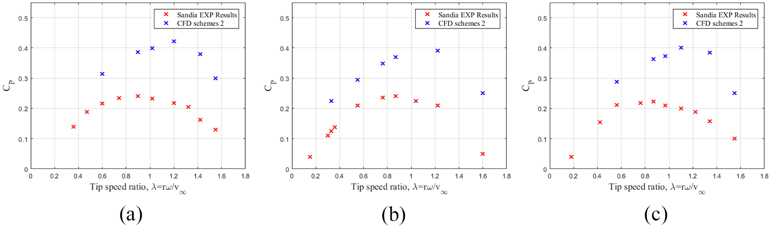
The first-order scheme is highly dissipative; when the turbulence increases with the tip speed ratio, this dissipation also increases, making the rotor to exchange less energy with the flow. Even that the results, in terms of $C_{P}$ , are close to the experimental values, the flow does not respond properly. This is why second-order schemes are considered and then compared. Figure 7 shows the results for second-order schemes and the experimental data.

Figure 7.

Experimental SANDIA (Blackwell et al., 1977) versus CFD results: second-order schemes: (a) OR = 10%, (b) OR = 15%, and (c) OR = 20%.

Second-order schemes

The first-order interpolation for the divergence discretization is stable but present poor accuracy due to numerical diffusion. This second configuration linear interpolation, a second-order scheme, is used. Even this scheme tends to be unstable; more accurate solution can be achieved. This modified schemes are less dissipative and also stability issues are more common and the time steps values are needed to be chosen and modified more carefully.

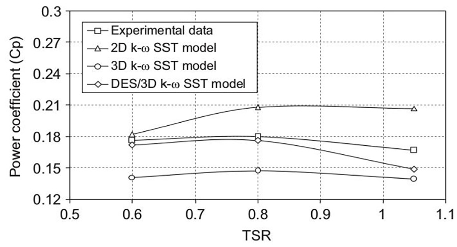
Dobrev and Massouh (2011) compared different CFD models with experimental data. This is shown in Figure 8. Despite this work do not detail the schemes used and very few $λ$ are simulated, the behavior of the 2D simulations are similar to the simulations made in this work using second-order time discretization.

Figure 8.

Models comparison by Dobrev and Massouh (2011).

Qualitative analysis

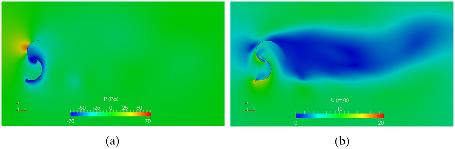
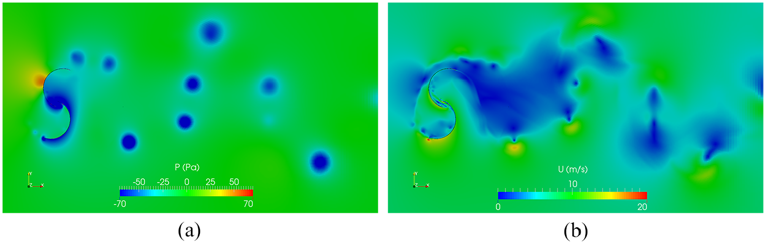
Besides the quantitative analysis regarding $C_{P}$ mean values for each operation condition, the velocity and pressure fields were observed. In Figures 9 and 10, the behavior of the flow is presented in terms of pressure and velocity. Both figures show the same case at the same time, but changing the solution schemes order. A high-pressure zone upstream and a low-pressure area downstream can be identified. The vortex shedding at the tip of the bucket produces high velocity and low pressure that propagate downstream, being gradually dissipated. From the comparison of first- and second-order schemes for the same case, it can be identified that the vortex shedding, mainly from the tip of the bucket, has different behavior. As it was said, the first-order upwind scheme is more dissipative, and it is confirmed by the differences shown in Figures 9 and 10, for the velocity and pressure fields.

Figure 9.

Pressure and velocity fields: first-order schemes: $OR = 15 %$ , $λ = 1.2$ , $u_{\infty} = 7 m / s$ : (a) pressure field and (b) velocity field.

Figure 10.

Pressure and velocity fields: second-order schemes: $OR = 15 %$ , $λ = 1.2$ , $u_{\infty} = 7 m / s$ : (a) Pressure field and (b) velocity field.

It can be noticed that the gap between buckets $(OR)$ has a significant influence in the flow behavior during the interaction with the rotor.

Domain analysis

Besides the grid size and the cells near the rotors walls, the size of whole domain affects the flow behavior and, therefore, the resulting $C_{P}$ . If the width is not big enough, the flow will be confined, acting like a guide vane and increasing the energy exchange between the flow and the rotor. On the contrary, if the distance to inlet or to the outlet is not properly dimensioned, the flow will not develop as it should, and the behavior will be affected by the boundary conditions apply to the inlet and outlet. This aspect is not carefully analyzed in the works found in the literature, and a wide range of domain sizes are used by the different authors. Rezaeiha et al. (2018) considers a domain width of 20 D, while 5 D and 25 D are considered for the distance to inlet and outlet respectively. Alom and Saha (2018) considers 6 D for the width and distance to outlet, while 4 D is used for the inlet distance. Ferrari et al. (2017) apply domains that extend 9 D upstream, 17 D downstream, and 12 D from side to side. For this study, different domains were generated and compared. With a domain as a reference case, the different dimensions were gradually increased. The first comparison is done to analyze the impact of the domain length. Table 1 shows the dimensions of three domains considered, where $D_{i}$ is the distance from the rotor to the inlet, $D_{o}$ to the outlet, and $D_{w}$ the domain width as it was shown in Figure 3. Figure 11 shows how the domain length affects the simulations behavior, in particular $C_{P}$ values. The domains have the same width, and the length is modified. In this case, the most significant variation is due to increasing the inlet distance, as it can be seen in results from domain 1 to 2.

Table 1.

Domain sizes in terms of rotor diameter.

	$D_{i}$	$D_{o}$	$D_{w}$
Domain 1	4.0 $D$	12.1 $D$	8.1 $D$
Domain 2	8.1 $D$	12.1 $D$	8.1 $D$
Domain 3	12.1 $D$	20.2 $D$	8.1 $D$

Figure 11.

Domain analysis.

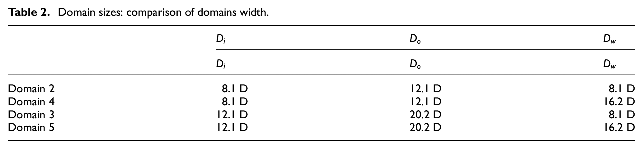
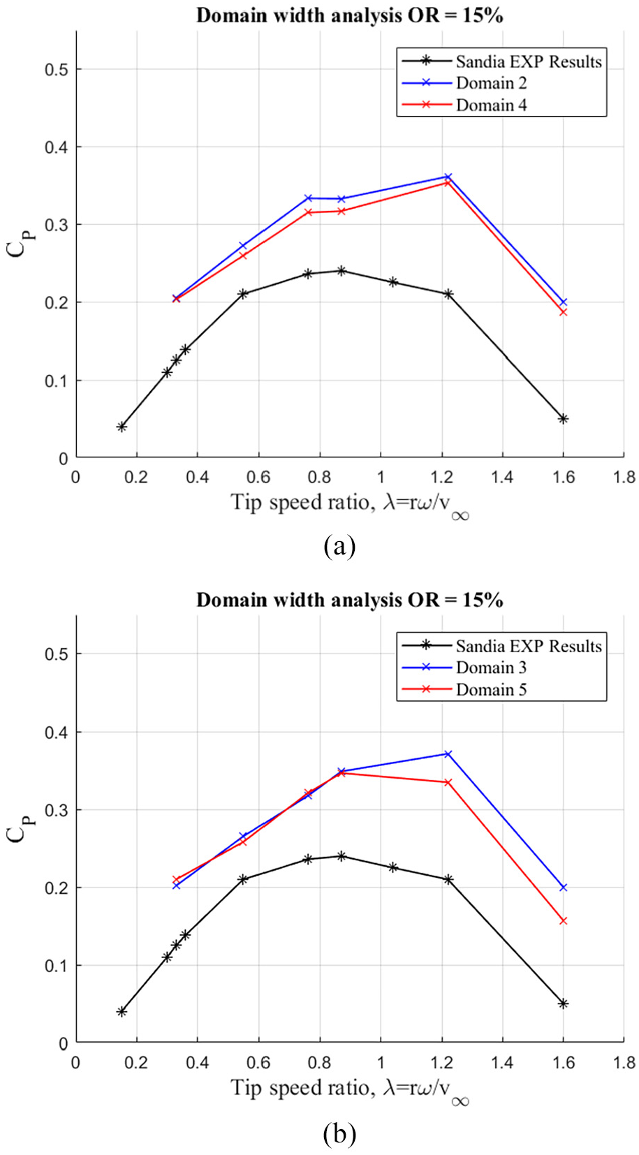
The impact of the domain width, $D_{w}$ , is analyzed comparing two pairs of cases (Domains 2 and 4, and Domains 3 and 5; the dimension of these domains are shown in Table 2. In each, the distance to the inlet and outlet is kept unaltered and the width is increased by a factor of two.

Table 2.

Domain sizes: comparison of domains width.

	$D_{i}$	$D_{o}$	$D_{w}$
	$D_{i}$	$D_{o}$	$D_{w}$
Domain 2	8.1 $D$	12.1 $D$	8.1 $D$
Domain 4	8.1 $D$	12.1 $D$	16.2 $D$
Domain 3	12.1 $D$	20.2 $D$	8.1 $D$
Domain 5	12.1 $D$	20.2 $D$	16.2 $D$

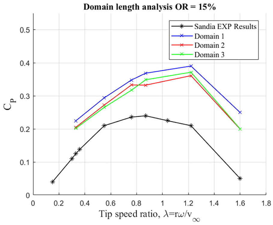
In Figure 12(a) and (b), the $C_{P}$ values decrease while $D_{w}$ increase.

Figure 12.

Comparison of CFD results increasing the domain width. (a) Domain width impact. D_i = 8.1 D and D_o = 12.1 D; (b) Domain width impact. D_i = 12.1 D and D_o = 20.2 D.

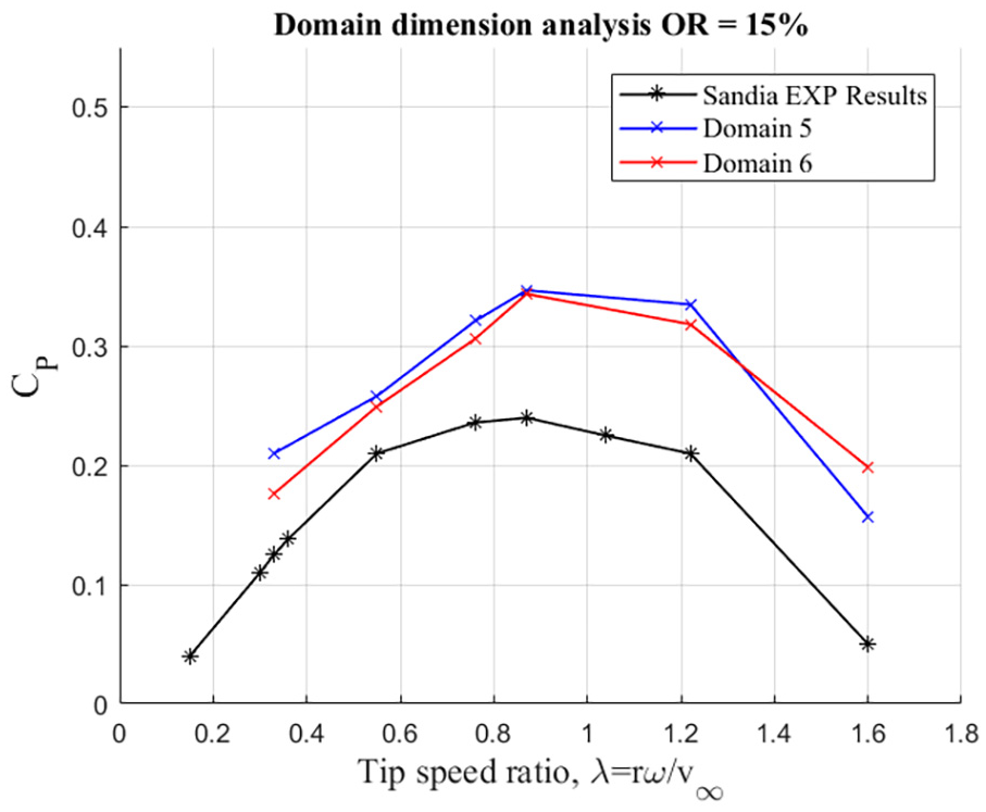
For both cases compared, the $C_{P}$ decrease as the grid is wider, getting closer to the experimental values. The Domain 5, with a grid size of $D_{i} = 12.1 D$ , $D_{o} = 20.2 D$ and $D_{w} = 16.2 D$ , shows the best results. In order to determine if this grid is big enough, and it does not generate unwanted effects due to the boundary conditions, another domain, bigger in all dimensions, is set and the results are compared in Figure 13.

Figure 13.

Comparison of CFD results increasing all domain dimensions.

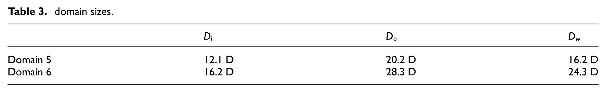
Finally, this sixth domain, bigger in all dimensions than Domain 5, is set and the simulations are made. Despite this, $C_{P}$ shows not significant variation from Domains 5 to 6. Their dimensions are shown in Table 3. This analysis conclude that a domain with $D_{i} = 12.1 D$ , $D_{o} = 20.2 D$ , $D_{w} = 16.2 D$ is necessary to avoid unwanted effects in the simulations of Savonius rotor geometries. Also, it is observed that these effects tend to increase $C_{P}$ values.

Table 3.

domain sizes.

	$D_{i}$	$D_{o}$	$D_{w}$
Domain 5	12.1 $D$	20.2 $D$	16.2 $D$
Domain 6	16.2 $D$	28.3 $D$	24.3 $D$

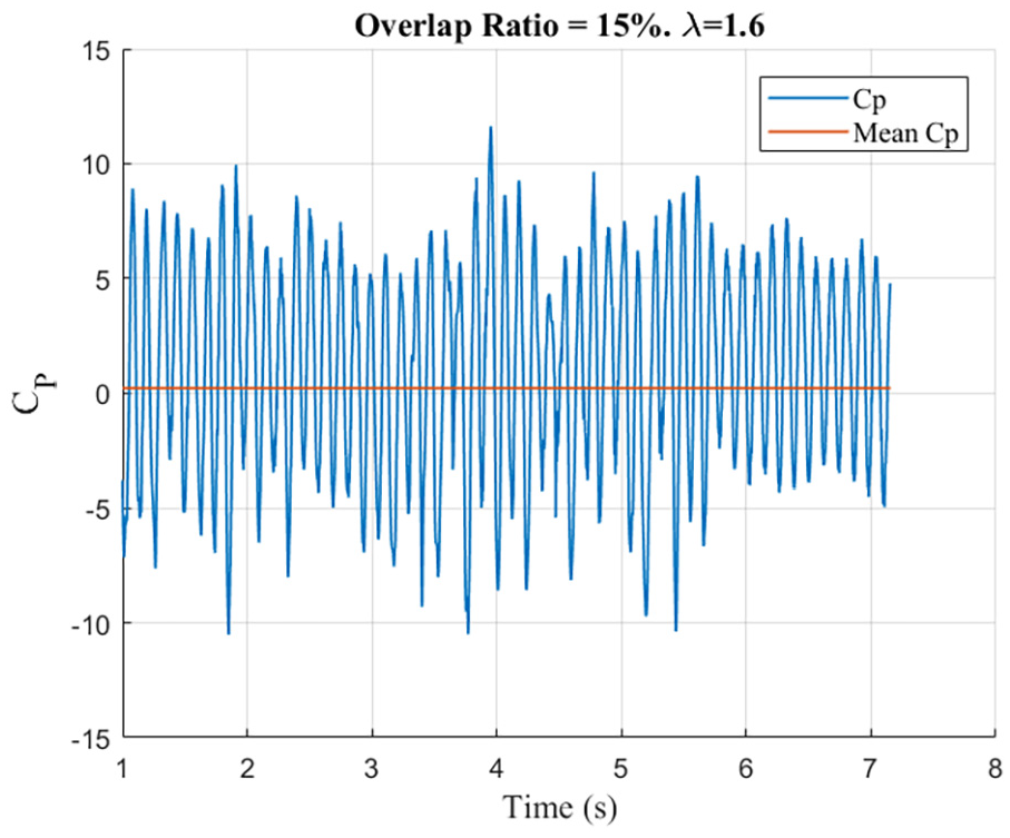
For higher values of tip speed ratio, there are some extra consideration to take into account for a proper analysis. In this condition (high $λ$ values), the flow is highly turbulent. Furthermore, this condition results in high fluctuations of $C_{P}$ , with a mean value close to $0$ . Figure 14 shows high fluctuation of $C_{P}$ over time and over its mean value. $C_{P}$ comparisons for high $λ$ values should be made carefully, since this values are highly disperse and the mean value is not significant to made certain comparisons.

Figure 14.

$C_{P}$ over time for high tip speed ratio $(λ = 1.6)$ . $OR = 15 %$ , $u_{\infty} = 7 m / s$ .

The requirements determined for the domain size could change significantly for other types of rotors, and a specific analysis could be necessary. For example, Darrieus rotors have less area blocked by the rotor, and it is expected that a smaller domain is required.

The domain width in CFD simulations could be considered as the cross area of a wind tunnel where a model is tested. Jeong et al. (2018) and Roy and Saha (2014) consider that $5 %$ – $7 %$ is the area that can be occupied for a model without need for a blockage correction factor. Taking this consideration for 2D simulations, the width of the domain should be $5 %$ to $7 %$ of the rotor diameter, or in terms of diameters, $20 D$ to $14.3 D$ . The previous analysis show that a width of 16.2 D adequate for the consider CFD cases, being consistent with the blockage consideration for wind tunnel tests. This domain can have a significant impact on the results of the simulations, especially for high tip speed ratios. The $C_{P}$ for tip speed ratio of 1.22 varies as much as $25.4 %$ from the smallest domain to the bigger one.

Results summary

The previous sections show a comparison between first- and second-order discretization schemes, and the influence of domain size on the results. Second-order discretizations capture the development of the flow in detail, and an adequate domain size is found so that the results are not affected by it. This domain, with dimensions $D_{i} = 12.1 D$ , $D_{o} = 20.2 D$ and $D_{w} = 16.2 D$ , is considerably broader than those used in some similar works found in the references. Figure 15 shows the results under these modeling conditions, using 2D URANS with turbulence equations given by $k - ω$ SST and with the PIMPLE solver. The time step was adjusted for the rotor advance less than 1° in the azimuth position for every, case. This is, $Δ θ < 1 °$ in each time step.

Figure 15.

Results for $C_{P}$ : $OR = 15 %$ , Domain 5, second discretization schemes.

To improve the results obtained, it would be necessary to venture into 3D models, with the complexity and computational cost that these imply. Ferrari et al. (2017) perform some 3D CFD modeling for Savonius rotors and compare these results with others in 2D and the same experimental results used as reference in this work (Blackwell et al., 1977).

Fluid–rotor interaction analysis

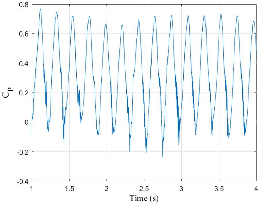
The physical phenomenon that occurs while the rotor rotates at a constant speed and the fluid travels with a speed imposed on the inlet is highly turbulent and unstable. This is simulated with the URANS turbulence model and the OpenFOAM solver PIMPLE, capable of capture these non-stationary characteristics. In the first moments of the simulation, just under 1 s, the fluid and the rotor begin to interact, and it is after this time that essentially periodic behavior is achieved. Nevertheless, a variability is maintained between each rotation cycle of the rotor. The vortex detachment and its evolution is not exactly repetitive. The Figure 16 shows the evolution of the power coefficient after the first second of simulation, where these cyclical characteristics are observed but not exact due to instabilities.

Figure 16.

$C_{P}$ versus time for $λ = 0.87$ , $OR = 15 %$ , and $u_{\infty} = 7 m / s$ .

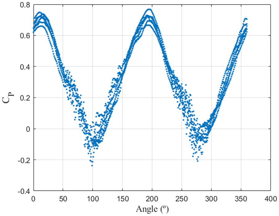
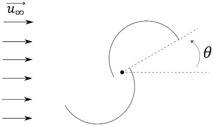
In the simulations, fluid velocity upstream of the rotor is imposed $(u_{\infty})$ , as well as the speed of rotation of the rotor $(ω)$ , which means that each instant of time corresponds to an angular position in the rotation of the rotor. The results of the fluid–rotor interaction are shown in Figures 17 and 18 in terms of the power coefficient $C_{P}$ . Several cycles are fulfilled for the simulated time and the results of all of them are presented in these figures, obtaining several values for each angle $θ$ . The position with angle $0 °$ corresponds to the rotor located so that the line that divides the Savonius rotor blades are parallel to the fluid, while the rotor advances its rotation counterclockwise (Figure 19). The detail of the position with the angle and the resulting pressure field is observed in Figure 20.

Figure 17.

$C_{P}$ versus $θ$ . $λ = 0.87$ , $OR = 15 %$ , $u_{\infty} = 7 m / s$ .

Figure 18.

$C_{P}$ versus $θ$ polar. $λ = 0.87$ , $OR = 15 %$ , $u_{\infty} = 7 m / s$ .

Figure 19.

Wind direction and angular position.

Figure 20.

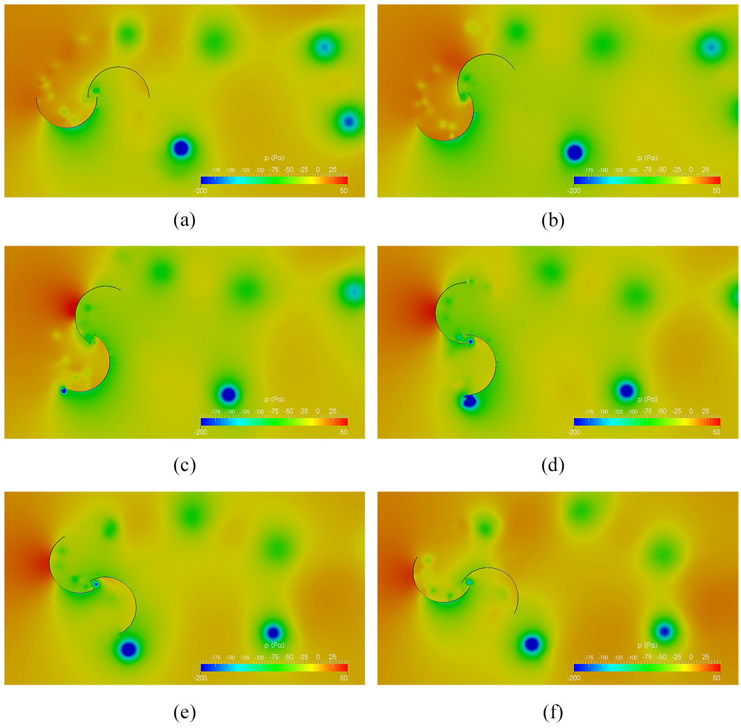
Pressure field results: second-order discretization schemes, Domain 5. $OR = 15 %$ , $λ = 0.87$ , $u_{\infty} = 7 m / s$ : (a) angular position (0°), (b) angular position (30°), (c) angular position (60°), (d) angular position (90°), (e) angular position (120°), and(f) angular position (150°).

The results of $C_{P}$ as a function of the angular position, $θ$ , shows that the highest instantaneous power coefficients occur at approximately $10 °$ , while the minimum results at $100 °$ , a quarter of a turn after the maximum. Then, it increase again to this maximum after completing another quarter of a turn. After this, the behavior is repeated, as expected considering that the rotor is symmetrical.

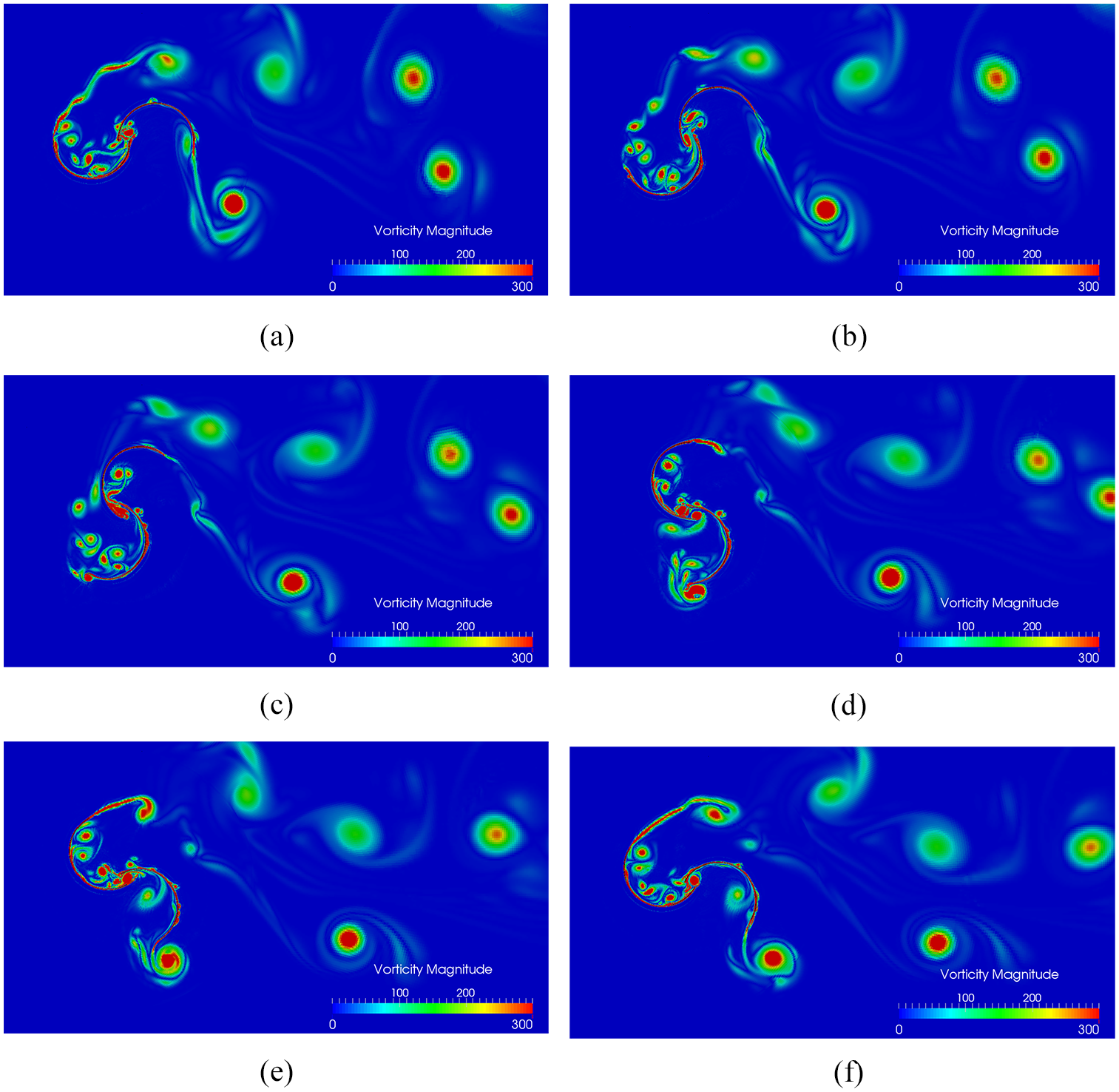
The minimum $C_{P}$ values are negatives, what implies that the rotor consume energy to overcome the angular positions near this point. It is also distinguished by observing Figure 17 that there is greater dispersion of the results in these positions than in the rest of the cycle. To analyze these points, the simulation fields results for different positions are extracted. Figure 19 schematically shows the wind direction and the angular position of the rotor in the simulations. For different angular positions, $θ$ , Figures 20 and 21 show the pressure and the vorticity in magnitude. The vortex that are generated in the fluid passage through the rotor and propagate downstream are seen as areas with high vorticity and are also distinguished as areas of low pressure. When the rotor passes 100°, these vortex detach from both blades. These vortex shedding are related to negative power coefficients, and they are erratic and variable, resulting in the dispersion observed in Figure 17 for $C_{P}$ values.

Figure 21.

Vorticity field results: second-order discretization schemes, Domain 5: $OR = 15 %$ , $λ = 0.87$ , $u_{\infty} = 7 m / s$ : (a) angular position (0°), (b) angular position (30°), (c) angular position (60°), (d) angular position (90°), (e) angular position (120°), and(f) angular position (150°).

Vortex shedding at the tips of the blades is associated with low values of $C_{P}$ . Furthermore, for such detachments, there is high variability in the results from one cycle to another. As noted before, there are not many studies that model Savonius rotors using CFDs, but in the case of Darrieus models, there are more studies and with more detail. Some works relate these detachments, the vortex generation, with the values of $C_{P}$ the rotor power coefficient for different angles. Qamar and Janajreh (2017) and Souaissa et al. (2019) model Darrieus using CFD and although the behavior differs in some aspects, it is corroborated that the minimum values of $C_{P}$ corresponds to the highest vortex shedding zone. Bianchini et al. (2017) also shows CFD results and comparisons with wake experiments for a three-bladed Darrieus rotor. In the studies presented by Chowdhury et al. (2016) and Hand and Cashman (2018), two-bladed Darrieus rotors are modeled and analyzed, allowing for a closer analogy to the Savonius rotor discussed in this article. Both works show the same relationships between vorticity generation and $C_{P}$ minimums. In Hand and Cashman’s (2018) work, the two-bladed Darrieus rotor has a 0 Â° angular position when the two blades are joined by a perpendicular to the flow velocity. It is near this position (approximately 10° or 15°) where the greatest vortex detachments occur and, therefore, the minimum $C_{P}$ .

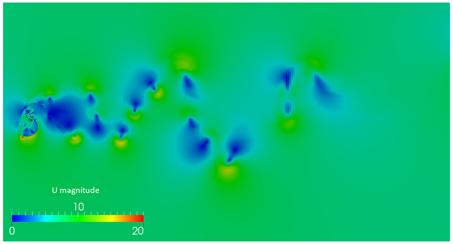
Figure 22 shows the results obtained for the vorticity. A region behind the rotor is observed, which has high vorticity and low speed. As expected for this region (wake of the wind turbine), it expands downstream at the same time that the vorticity dissipates and the speed approaches to the flow without disturbances. This dynamic can also be seen in Figure 23.

Figure 22.

Wake vorticity field: $OR = 15 %$ , $λ = 0.87$ , $u_{\infty} = 7 m / s$ .

Figure 23.

Wake velocity field: $OR = 15 %$ , $λ = 0.87$ , $u_{\infty} = 7 m / s$ .

Conclusion

A systematic sensitivity analysis is performed using URANS simulations to provide accurate results for the 2D CFD simulation of Savonius rotors. Grid size, domain size, and numerical resolution schemes for different tip speed ratios and ORs are analyzed and compared. The evaluation is based on validation with wind-tunnel measurements for VAWTs (Blackwell et al., 1977).

First-order schemes for time derivative and spatial gradient results in a too dissipative flow, especially for high tip speed ratio values. For these operation points, $C_{P}$ values are lower than experimental results even that the simulations are $2 D$ and expected to over-predict the power coefficient. By flow visualizations can be confirmed this conclusion, since the simulations cannot capture the flow phenomena in detail. Second-order schemes ensure that the flow complexities such turbulence, vortex shedding, and bucket-wake interactions are accurately predicted.

The domain size results to impact dramatically in the prediction of $C_{P}$ . While there are some works about CFD domain size for Darrieus rotors, this is not the case for Savonius rotors, and its geometry and interaction with the flow is quite different. The domain size comparison results that the minimum distance from the turbine center to the domain inlets needs to be $12.1 D$ . This values ensures that for every tip speed ratio and OR consider, the domain contains adequately the turbine upstream field. A distance to the outlet of $20.2 D$ ensures that the turbine wake is developed properly, and therefore, the domain has no impact in the results.

The domain width is also analyzed. As it occurs with the blockage effect in a wind tunnel, if the domain is not wider enough, the flow is confined resulting in higher values in the turbine performance. It was found that a domain width of $16.2 D$ is necessary to ensure that the blockage effects negligible. In this way, the rotor takes a $6.2 %$ of the domain width. This value is consistent with the experimental recommendations for blockage in several studies, which consider values no grater than $5 %$ or $7 %$ of the wind tunnel area are necessary to neglect blockage effects.

The analysis of the wake and instantaneous $C_{P}$ values shows correlations. When the vortex shedding is more intense, the minimum values of $C_{P}$ are reached. These results and the wake behavior is consistent with some analogue studies cited in the bibliography.

Footnotes

Acknowledgements

The authors would like to acknowledge support from the Uruguayan agency of innovation and research (ANII) through the program “Fondo Sectorial de Energía” (project: “Viento que ilumina. Diseño y fabricación de prototipos de micro aerogeneradores para iluminación” FING-ANII-FSE-102560.), which partially supports the present work. F.G.M. is grateful for his scholarship granted by ANII, whose thesis is related to the present work.

Declaration of conflicting interests

The author(s) declared no potential conflicts of interest with respect to the research, authorship, and/or publication of this article.

Funding

The author(s) received no financial support for the research, authorship, and/or publication of this article.

References

Akwa

da Silva Júnior

Petry

(2012) Discussion on the verification of the overlap ratio influence on performance coefficients of a Savonius wind rotor using computational fluid dynamics. Renewable Energy 38(1): 141–149.

Al-Faruk

Sharifian

(2017) Flow field and performance study of vertical axis Savonius type SST wind turbine. Energy Procedia 110: 235–242.

Alom

Saha

(2018) Performance evaluation of vent-augmented elliptical-bladed Savonius rotors by numerical simulation and wind tunnel experiments. Energy 152: 277–290.

Bianchini

Balduzzi

Bachant

, et al. (2017) Effectiveness of two-dimensional CFD simulations for Darrieus VAWTs: A combined numerical and experimental assessment. Energy Conversion and Management 136: 318–328.

Blackwell

Sheldahl

Feltz

(1977) Wind tunnel performance data for two-and three-bucket Savonius rotors. Report No. SAND76-0131, July 1977. Springfield, VA: Sandia National Laboratories.

Chauvin

Botrini

Brun

, et al. (1983) The evaluation of the power coefficient of a Savonius rotor. Academie des Sciences Paris Comptes Rendus Serie Sciences Mathematiques 296: 823–826.

Chowdhury

Akimoto

Hara

(2016) Comparative CFD analysis of vertical axis wind turbine in upright and tilted configuration. Renewable Energy 85: 327–337.

Dobrev

Massouh

(2011) CFD and PIV investigation of unsteady flow through Savonius wind turbine. Energy Procedia 6: 711–720.

El-Askary

Nasef

Abdel-Hamid

, et al. (2015) Harvesting wind energy for improving performance of Savonius rotor. Journal of Wind Engineering and Industrial Aerodynamics 139: 8–15.

10.

Ferrari

Federici

Schito

, et al. (2017) CFD study of Savonius wind turbine: 3D model validation and parametric analysis. Renewable Energy 105: 722–734.

11.

González

Cataldo

(2019) Estudios de viabilidad para la microgeneración eólica en ambientes urbanos. Congreso de Agua Ambiente y Energía. AUGM. Montevideo, Uruguay.

12.

Gupta

Biswas

Sharma

(2008) Comparative study of a three-bucket Savonius rotor with a combined three-bucket Savonius–three-bladed Darrieus rotor. Renewable Energy 33(9): 1974–1981.

13.

Hand

Cashman

(2018) Aerodynamic modeling methods for a large-scale vertical axis wind turbine: A comparative study. Renewable Energy 129: 12–31.

14.

Jeong

Lee

Kwon

(2018) Blockage corrections for wind tunnel tests conducted on a Darrieus wind turbine. Journal of Wind Engineering and Industrial Aerodynamics 179: 229–239.

15.

Jian

Kumbernuss

Linhua

, et al. (2012) Influence of phase-shift and overlap ratio on Savonius wind turbine’s performance. Journal of Solar Energy Engineering 134(1): 011016.

16.

Kacprzak

Liskiewicz

Sobczak

(2013) Numerical investigation of conventional and modified Savonius wind turbines. Renewable Energy 60: 578–585.

17.

Marmutova

(2016) Performance of a Savonius wind turbine in urban sites using CFD analysis. Available at: https://www.univaasa.fi/materiaali/pdf/isbn_978-952-476-675-3.pdf

18.

Menter

(1993) Zonal two equation kw turbulence models for aerodynamic flows. In: Proceedings of the 23rd fluid dynamics, plasmadynamics, and lasers conference, Orlando, FL, 6–9 July 1993, p. 2906. Reston, VA: American Institute of Aeronautics and Astronautics.

19.

Modi

Fernando

(1993) Unsteady aerodynamics and wake of the Savonius wind turbine: A numerical study. Journal of Wind Engineering and Industrial Aerodynamics46–47: 811–816.

20.

Mojola

(1985) On the aerodynamic design of the Savonius windmill rotor. Journal of Wind Engineering and Industrial Aerodynamics 21(2): 223–231.

21.

Moukalled

Mangani

Darwish

, et al. (2016) The Finite Volume Method in Computational Fluid Dynamics: An Advanced Introduction With OpenFoam^® and Matlab. New York: Springer.

22.

Nasef

El-Askary

Abdel-Hamid

, et al. (2013) Evaluation of Savonius rotor performance: Static and dynamic studies. Journal of Wind Engineering and Industrial Aerodynamics 123: 1–11.

23.

Paraschivoiu

(2002) Wind Turbine Design: With Emphasis on Darrieus Concept. Montreal, QC, Canada: Presses inter Polytechnique.

24.

Qamar

Janajreh

(2017) A comprehensive analysis of solidity for cambered Darrieus VAWTs. International Journal of Hydrogen Energy 42(30): 19420–19431.

25.

Rezaeiha

Montazeri

Blocken

(2018) Towards accurate CFD simulations of vertical axis wind turbines at different tip speed ratios and solidities: Guidelines for azimuthal increment, domain size and convergence. Energy Conversion and Management 156: 301–316.

26.

Roy

Saha

(2014) An adapted blockage factor correlation approach in wind tunnel experiments of a Savonius-style wind turbine. Energy Conversion and Management 86: 418–427.

27.

Shaheen

El-Sayed

Abdallah

(2015) Numerical study of two-bucket Savonius wind turbine cluster. Journal of Wind Engineering and Industrial Aerodynamics 137: 78–89.

28.

Souaissa

Ghiss

Chrigui

, et al. (2019) A comprehensive analysis of aerodynamic flow around H-Darrieus rotor with camber-bladed profile. Wind Engineering 43(5): 459–475.

29.

Vignolo

Narbondo

Cataldo

, et al. (2015) Feasibility studies for the instalation of wind microgeneration in urban areas in Montevideo. In: Proceedings of the 2015 IEEE PES innovative smart grid technologies Latin America (ISGT LATAM), Montevideo, Uruguay, 5–7 October 2015, pp. 734–739. New York: IEEE.

30.

White

(2003) Fluid Mechanics. New York: McGraw-Hill.