Frequency support scheme based on parametrized power curve for de-loaded wind turbine under various wind speed

Abstract

With increased wind power penetration in modern power systems, wind plants are required to provide frequency support similar to conventional plants. However, for the existing frequency regulation scheme of wind turbines, the control gains in the auxiliary frequency controller are difficult to set because of the compromise of the frequency regulation performance and the stable operation of wind turbines, especially when the wind speed remains variable. This paper proposes a novel frequency regulation scheme (FRS) for de-loaded wind turbines. Instead of an auxiliary frequency controller, frequency support is provided by modifying the parametrized power versus rotor speed (P_w-ω_r) curve, including the inertia power versus rotor speed curve and the droop power versus rotor speed curve. The advantage of the proposed scheme is that it does not contain any control gains and generally adapts to different wind speeds. Further, the proposed scheme can work for the whole section of wind speed without wind speed measurement information. The compared simulation results demonstrate the scheme improves the system frequency response while ensuring the stable operation of doubly-fed induction generators (DFIGs)-based variable-speed wind turbines (VSWTs) under various wind conditions. Furthermore, the scheme prevents rotor speed overdeceleration even when the wind speed decreases during frequency regulation control.

Keywords

DFIGs frequency support inertia control power versus rotor speed curve de-loaded control the whole wind speed section

Introduction

Wind power generation is the most popular renewable generation technology, and the technology of wind turbine is still improving (Singh and Sundaram, 2020; Singh et al., 2019b, 2021), such as the improvement of wind turbine cooling system (Singh and Sundaram, 2021; Singh et al., 2018, 2019c), fault analysis (Singh et al., 2019a, 2019d), and so on. In 2020, the new installation of wind power generation was 93 GW, and the total installed capacity was 743 GW (Global Wind Energy Outlook, 2020). Approximately 95% of installed wind turbines (WTs) are Variable speed wind turbines (VSWTs), either DFIGs-based with partially rated converters or PMSGs-based with fully rated converters (Babu and Ramesh, 2013; Liserre et al., 2011). Unlike conventional power generators, VSWTs have no inherent inertial response because of the power electrical converter interface. VSWTs usually do not participate in the system frequency response for operation in maximum power point tracking (MPPT) mode. Therefore, as the penetration of VSWTs increases, the inertial and frequency regulation ability of the whole power system will degrade, causing frequency stability issues (Liu et al., 2017; Margaris et al., 2012). Some countries have required wind plants to provide frequency support (Aho et al., 2012; Hydro Québec, 2009; Nordic Grid Code, 2007).

Many research studies have discussed the frequency regulation scheme (FRS) for VSWTs. The strategies can be classified into inertial response control and de-loaded control (Wu et al., 2018, 2019).

For inertial response control, the VSWTs still operate in MPPT mode, and the rotational kinetic energy (KE) of VSWTs is released to deliver temporary addition power during frequency dips. Further, the inertial response control can divide in two subcategories (Wu et al., 2019): natural inertial control (Kayikçi and Milanovic, 2009; Lee et al., 2016; Min et al., 2016; Morren et al., 2006; Wu et al., 2019; Zhao et al., 2015, 2020) and stepwise control (Hafiz and Abdennour, 2015; Kang et al., 2016; Ullah et al., 2008).

For natural inertial control, the value of the addition power is determined by the frequency measurement, such as the rate of change of frequency (ROCOF) (Kayikçi and Milanovic, 2009), or the frequency deviation (Lee et al., 2016; Morren et al., 2006), or both of them (Lee et al., 2016; Min et al., 2016; Wu et al., 2019; Zhao et al., 2015, 2020). Considering that the wind speed is variable and the change of the rotor speed is complicated, the auxiliary frequency controller’s gains should be selected carefully with the trade-off considering the frequency regulation performance and the stable operating range of the wind turbine. Therefore, some varying gain methods have been suggested. In Zhao et al. (2015), the control gains of FRS under different wind speeds is adjusted based on the wind speed. However, the pre-determined gains are obtained by the off-line modeling analysis, and the wind speed measurement may not be obtained or inaccuracy. To improve the frequency nadir (FN) and ensure stable operation of DFIG, the droop gains is dynamically changes based on ROCOF in Min et al. (2016). In Lee et al. (2016), the gains of additional ROCOF and frequency deviation loops is adaptively tuned depended on the rotor speed measurement. Wu et al. (2019) present a time varying gains determined based on desired frequency-response time to raise frequency nadir and eliminate frequency second dip. Zhao et al. (2020) proposed an adaptive droop gain which is a function of real-time rotor speed and wind power penetration level.

For step-wise control, the addition frequency power is determined by the pre-set power surge function, such as step function (Ullah et al., 2008), ramp function (Hafiz and Abdennour, 2015), or torque limit function (Kang et al., 2016). Compared with natural inertial response, the inertial power using the step-wise control can be properly tuned according to different shapes in terms of its magnitude and duration. An optimization approaches employing the genetic algorithm are proposed to maximize the released energy from the wind turbine during its overproduction period (Altin et al., 2018). However, during the rotor speed recovery period, the output power of wind turbine reduced and may cause a secondary frequency drop (Yang et al., 2018a, 2018b). In Yang et al. (2018a, 2018b), the incremental power varies with the rotor speed and wind power penetration levels during the overproduction period, and then, the reference power smoothly decreases with time and rotor speed during recovery period.

For inertial response control, because of the limit of the rotor kinetic energy, it only affords for seconds-term frequency support. While, for the de-loaded control, VSWTs reserve a part of the active power through pitch angle control (Margaris et al., 2012; Wu et al., 2018), over-speed control (Chang-Chien et al., 2011), or combination of both (Luo et al., 2019; Tang et al., 2019; Zertek et al., 2012). It can provide a minutes-term primary frequency support.

Due to rotor speed limit, the over-speed de-loaded control is only adapted for low wind range. In Zhang et al. (2012) and Li et al. (2019), three wind speed modes are defined: low wind speed mode where de-loaded operation is merely by rotor speed control; medium wind speed mode where de-loaded operation is conducted by combining pitch angle control and rotor speed control; and high wind speed mode where modified pitch angle control alone. However, it required accuracy wind speed information to judge the wind speed mode, and the calculation of de-loaded power reference need both parameters of wind turbine and wind speed. Liu et al. (2019) present a variable droop control strategy that considers optional rotor kinetic energy. However, the rotor kinetic energy estimation required the wind speed information and parameters of wind turbine. Wang and Tomsovic (2018) proposed a comprehensive frequency control that combines the temporary power injection control and power reserve control with consider rotor security and maximum extricable energy of wind turbines. But, it still required the parameter of wind turbines. In Gao et al. (2019) a comprehensive frequency regulation that combines the step-wise inertial control and variable-droop control is present.

Actually, in most of the literatures mentioned above, the additional frequency regulation power is determined by an auxiliary ROCOF and frequency deviation loops, which is added to the de-loaded power reference. The gains of the auxiliary frequency controller are difficult to set a proper value compromising of the frequency regulation performance and wind turbines rotor security. Moreover, if these schemes are applied to multiple WTGs, difficulties will arise in determining the different gains for all WTGs. Nevertheless, some adaptive gains methods in Lee et al. (2016), Liu et al. (2019), Min et al. (2016), Wang and Tomsovic (2018), Wu et al. (2019), Zhao et al. (2015, 2020), the proper initial value or parameters are also difficult to select (Lee et al., 2016; Min et al., 2016; Wu et al., 2019; Zhao et al., 2015, 2020), or the gains are determined by evaluating available energy which of the accurate parameters of wind turbines and wind speed information are required (Liu et al., 2019; Wang and Tomsovic, 2018).

This paper proposes a novel frequency support scheme for DFIG-based wind turbines. Instead of the auxiliary frequency controller in the most existing scheme, the additional frequency regulation power for wind turbines is determined by the modified parametrized power versus rotor speed curve. There are three main advantages of the proposed control scheme:

There are no control gains in the scheme. Thus, it does not need to carefully select a proper control gains for wind turbines like the existing scheme. It can generally adapt for multiple WTGs with different wind speeds.

It has potential self-adaptive frequency support with wind speed and can continuously ensure that the wind turbine operates within the safe rotor speed range, even in the case of a sudden decrease in wind speed.

It can work for the whole wind speed range and does not need wind speed information.

The remainder of this paper is organized as follows: In Section 2, the DFIG-based wind turbine model and the traditional frequency regulation scheme are introduced. In Section 3, the proposed frequency regulation scheme for DFIG-based wind turbines is presented. In Section 4, compared with the traditional frequency regulation, the proposed control scheme’s performance is demonstrated under various wind conditions. Finally, a brief conclusion is drawn in Section 5.

DFIG model of a DFIG-based wind generation

Figure 1 shows the block diagram of DFIG-based wind turbines’ simplified model, commonly used for frequency control studies and developed in Ochoa and Martinez (2017). The mechanical power of a DFIG captured from the wind, P_m, is defined by (Sun et al., 2019)

P_{m} = \frac{1}{2} ρ π R^{2} {V_{W}}^{3} C_{p} (λ, β)

(1)

where ρ—air density, R—radius, V_w—wind speed, λ—tip speed ratio, λ = ω_rR/V_w, ω_r—rotor speed, β—pitch angle, and Cp(λ, β)—power coefficient.

Figure 1.

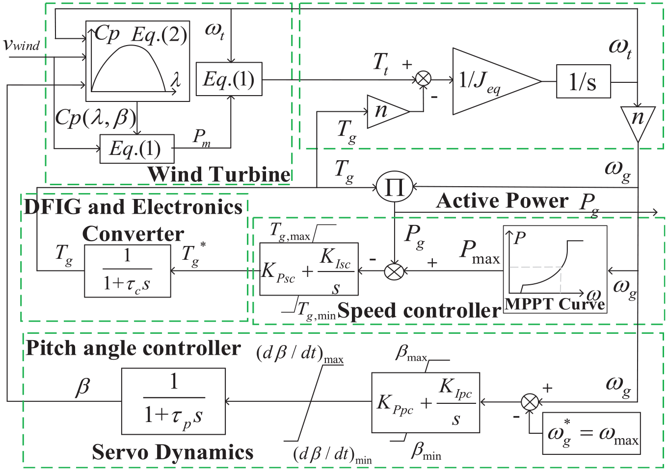
Block diagram of a simplified model of a DFIG-based wind turbine.

As in Ekanayake and Jenkins (2004), C_p(λ, β) can be expressed as:

C_{p} (λ, β) = (0.44 - 0.0167 β) \sin [\frac{π (λ - 3)}{5 - 0.3 β}] - 0.00184 (λ - 3) β

(2)

A “one mass” system has been considered to represent the rotational dynamics of the gearbox, wind turbine and electrical generator (Clark et al., 2010; Li et al., 2019), whose equivalent moment of inertia is J_eq. where T, P, and ω represent torque, power, and angular speed, respectively; subscripts g and t are used to indicate the variables referring to the generator and the turbine. fs, p, and n are the grid frequency, the number of pole pairs, and the gear ratio of the DFIG, respectively.

In addition, the DFIG and the rotor side converter (RSC) are both regarded as a single first-order dynamics actuator, with a time constant τ_C, whose input is the electromagnetic reference torque from the speed control system T_g^*.

Maximum power point tracking controller (MPPT)

To capture the maximum wind power by the wind turbine, a power reference, P_max is from the maximum power versus rotor speed (P_max-ω_r) curve that can be represented by (3) and illustrated in Figure 2 (the solid black line).

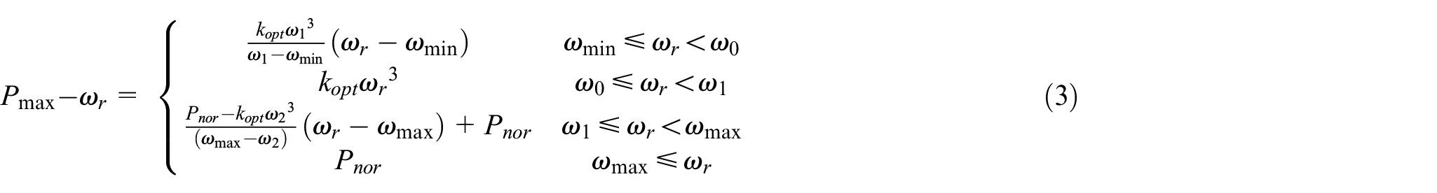
P_{max} - ω_{r} = {\begin{matrix} \frac{k_{opt} {ω_{1}}^{3}}{ω_{1} - ω_{min}} (ω_{r} - ω_{min}) & ω_{min} \leq ω_{r} < ω_{0} \\ k_{opt} {ω_{r}}^{3} & ω_{0} \leq ω_{r} < ω_{1} \\ \frac{P_{nor} - k_{opt} {ω_{2}}^{3}}{(ω_{max} - ω_{2})} (ω_{r} - ω_{max}) + P_{nor} & ω_{1} \leq ω_{r} < ω_{max} \\ P_{nor} & ω_{max} \leq ω_{r} \end{matrix}

(3)

where k_opt is the optimization constant, whose value depends on the physical characteristics of the wind turbine.

Figure 2.

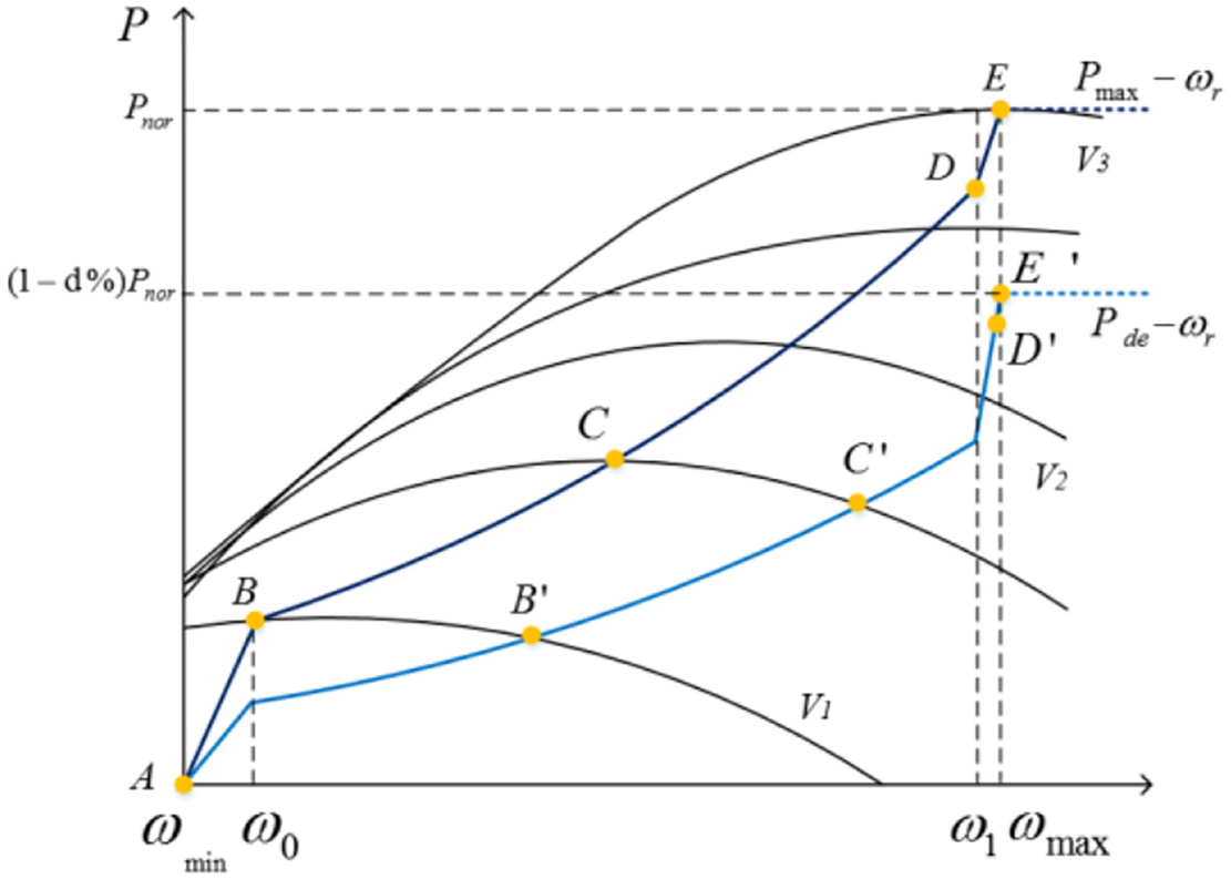
Maximum power curve and de-loaded power curve for DFIG-based VSWTs.

Concerning Figure 2, the maximum power curve is divided into four segments according to the rotor speed. The segment A–B corresponds to the starting zone. In segment B–D, known as the optimization zone, the rotor speed is adjusted to the optimal speed with the optimal power coefficient C_p(λ, β). Segments D–E are constant rotor speed zones, and the rotor is almost invariable. After the segment after point E is called the constant power zone, P_max is constant P_nor.

The intersection point of the capture power versus rotor speed curve (P_m-ω_r) and the maximum power curve (P_max-ω_r) is an equilibrium point. After some disturbances, the DFIG-WT automatically converges to the intersection point, where the captured mechanical power P_m is equal to the optimum power P_opt, and the rotor equals ω_opt.

A pitch-angle controller is used to prevent the rotor speed from exceeding ω_max and keep the output power at the rated value when wind speeds are high.

The traditional FRS for DFIG-based WT

The most popular FRS for wind turbines is shown in Figure 3, as in Lee et al. (2016) (and similar schemes in Lee et al. (2016), Luo et al. (2019), Min et al. (2016), Tang et al. (2019), Wu et al. (2019), Zertek et al. (2012), Zhao et al. (2015, 2020)). To realize de-loaded control, a de-loaded power versus rotor speed curve (P_de-ω_r) replaces the P_max-ω_r curve. This makes the rotor speed higher than the optimum rotor speed. The DFIG-WT operates at a suboptimal point below the maximum power point (reserve a part of the active power). A typical P_de-ω_r curve is given in Figure 2 (the blue line).

Figure 3.

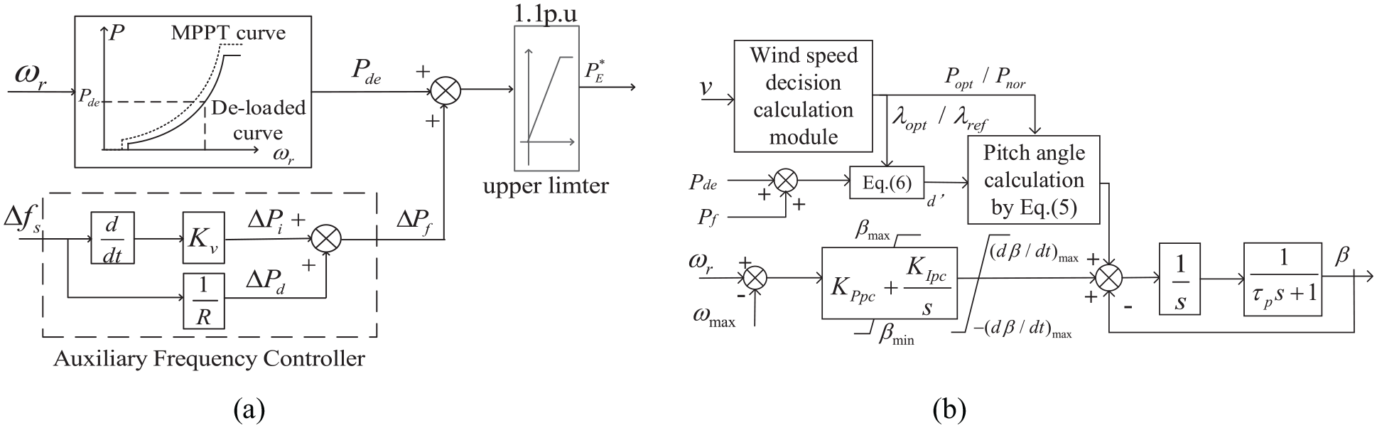
The commonly used frequency regulation controller for DFIG-based wind turbine: (a) auxiliary frequency controller (b) pitch angle controller.

An auxiliary frequency controller (AFC) is added to generate an additional power ΔP_f, as expressed in (4). It includes virtual inertia response and droop response. The inertia response is based on the ROCOF, while the droop response is based on the frequency deviation.

Δ P_{f} = K_{v} \cdot \frac{d Δ f_{s}}{dt} + \frac{1}{R} \cdot Δ f_{s}

(4)

where K_v and 1/R are the gains of the virtual inertia and droop loops, respectively.

The pitch angle control not only prevents the rotor speed from exceeding ω_max but also helps to realize de-loaded operation at medium and high wind speeds area (Lee et al., 2016). According to wind speed, the de-loaded control can be divided into three areas in Li et al. (2019), as shown in Figure 2.

Low wind speed area: V₁–V₂, β_de = 0, ω_r < ω_max; only the speed control loop is used to realize de-loaded control.

Medium wind speed area: V₂–V₃, β_de > 0, ω_r < ω_max. Both the speed control loop and pitch controller are used to realize de-loaded control.

High wind area: higher than V₃, β_de > 0, ω_r = ω_max, only the pitch controller is used to realize de-loaded control. β_de is the de-loaded pitch reference for avoiding overspeed.

The control of the pitch angle is shown in Figure 3(b). β_de is obtained from wind turbine modeling by solving equation (5).

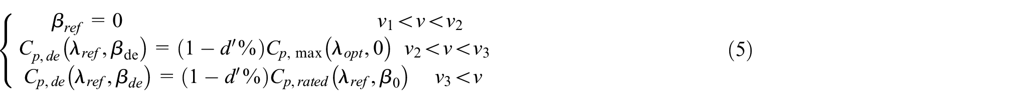
{\begin{matrix} β_{ref} = 0 v_{1} < v < v_{2} \\ C_{p, de} (λ_{ref}, β_{de}) = (1 - d' %) C_{p, max} (λ_{opt}, 0) v_{2} < v < v_{3} \\ C_{p, de} (λ_{ref}, β_{de}) = (1 - d' %) C_{p, rated} (λ_{ref}, β_{0}) \begin{matrix} v_{3} < v \end{matrix} \end{matrix}

(5)

where λ_opt is the optimum tip speed ratio and C_p_,max is the maximum wind energy capture factor. λ_ref is the reference tip speed ratio in over speed control, λ_ref = ω_maxR/v, and C_p_,rated is the wind energy capture coefficient when operating at rated power. β₀ is the pitch angle reference when the wind turbines operate at the rated power. β_de is the de-loaded pitch angle in the de-loaded control mode. d′% is the real de-loaded ratio of the wind turbine and can be calculated as:

d' = {\begin{matrix} 1 - \frac{P_{de} + Δ P_{f}}{P_{opt}}, v \leq V_{3} \\ 1 - \frac{P_{de} + Δ P_{f}}{P_{nor}}, v > V_{3} \end{matrix}

(6)

where P_opt is the reference power of the wind turbine under MPPT and P_nor is the rated power.

However, there are still some shortcomings for the traditional frequency regulation scheme.

The gains of AFC are challenging to set because of the compromise of the frequency support performance and wind turbines’ stable operation. A large gain can improve the frequency regulation while causing overdeceleration of a DFIG. Conversely, a small gain can prevent overdeceleration, but it provides a limited contribution to frequency supports. In addition, for multiple WTGs, the available energy is different because the available energy is determined by the wind turbine characteristics and wind speed. There cannot be a single proper value for all different DFIGs.

Wind speed information is required to realize de-loaded and frequency support control for the whole section of wind speed. As seen in Figure 3(b), wind speed information V is necessary for the decision of the wind speed area, calculating the maximum power P_opt and the optimum tip speed ratio λ_opt.

The proposed frequency regulation scheme

To address the limitations mentioned above, a novel frequency regulation scheme for de-loaded wind turbines is proposed. The whole control diagram of the proposed scheme is illustrated in Figure 4.

Figure 4.

The proposed frequency regulation scheme.

The proposed FRS includes two key steps. First, the de-loaded curve is modified into a droop power curve based on the frequency deviation to provide a droop frequency response. Second, the droop power curve is further modified into an inertia power curve based on ROCOF to provide both inertia and droop frequency responses. The detection of df_s/dt is sensitive to noise and harmonic disturbance. Hence, a washout filter (T_w = 0.01) (Wang et al., 2019) is used to obtain df_s/dt, as seen in Figure 4.

Then, the power reference P_E* can be obtained based on the measurement of the rotor speed ω_r.

The de-loaded power curve, the droop power curve and the inertia power curve are detailed below.

De-loaded power curve

The fixed power reserve d%, is defined as

d % = \frac{P_{opt} - P_{de}}{P_{opt}}

(7)

where P_opt is the maximum available power, P_de is the de-loaded power, and d% is set to 10% in the paper.

Similar to the P_max-ω_r curve, the de-loaded curve P_de-ω_r curve can be similarly expressed:

P_{de} - ω_{r} = {\begin{matrix} \frac{k_{de} {ω_{1}}^{3}}{ω_{1} - ω_{min}} (ω_{r} - ω_{min}) & ω_{min} \leq ω_{r} < ω_{0} \\ k_{de} {ω_{r}}^{3} & ω_{0} \leq ω_{r} < ω_{1} \\ \frac{0.9 P_{nor} - k_{de} {ω_{2}}^{3}}{(ω_{max} - ω_{2})} (ω_{r} - ω_{max}) + 0.9 P_{nor} & ω_{1} \leq ω_{r} < ω_{max} \\ 0.9 P_{nor} & ω_{max} \leq ω_{r} \end{matrix}

(8)

where k_de is the de-loaded constant and P_de is the de-loaded power.

Noticed that k_de does not equal the 0.9 k_opt. As shown in Figure 4, for the same wind speed, the rotor speed with 0.9 P_opt is larger than the optimum rotor speed. By off-line data fitting, it can be obtained that the value of k_de with a 10% power reserved ratio is 0.2172. At the maximum rotor speed for the de-loaded power curve, the corresponding wind speed is 10 m/s, instead of 12 m/s for the maximum power curve.

Droop power versus rotor curve

The droop power curve, P_droop-ω_r, is shifted from the de-loaded curve (P_de-ω_r) to the maximum power curve (P_max-ω_r) based on the frequency deviation.

d% is 10% in this paper, and the droop curve P_droop-ω_r is defined as follows:

P_{droop} - ω_{r} = {\begin{matrix} \frac{k_{sopt} {ω_{1}}^{3}}{ω_{1} - ω_{min}} (ω_{r} - ω_{min}) & ω_{min} \leq ω_{r} < ω_{0} \\ k_{sopt} {ω_{r}}^{3} & ω_{0} \leq ω_{r} < ω_{1} \\ \frac{((0.9 - 0.1 \frac{Δ f}{Δ f_{max}}) \cdot P_{nor} - k_{sopt} {ω_{1}}^{3})}{(ω_{max} - ω_{1})} (ω_{r} - ω_{max}) + P_{nor} & ω_{1} \leq ω_{r} < ω_{max} \\ (0.9 - 0.1 \frac{Δ f}{Δ f_{max}}) P_{nor} & ω_{max} \leq ω_{r} \end{matrix}

(9)

where k_sopt is defined as,

k_{sopt} = {\begin{matrix} k_{de} - (k_{opt} - k_{de}) \frac{Δ f}{Δ f_{max}} \begin{matrix} Δ f < 0 \end{matrix} \\ k_{de} - (k_{de} - k_{de}^{80 %}) \frac{Δ f}{Δ f_{max}} \begin{matrix} Δ f > 0 \end{matrix} \end{matrix}

(10)

Where k_de^80% is the de-loaded constant with an 80% power reserve for the wind turbine, which to provide 10% power regulation capability for frequency rise event. k_de^80% is obtains by off-line data fitting and k_de^80% = 0.1956. Δf_max is the allowable frequency deviation and Δf_max = 0.5 Hz in this paper.

The droop power curve is illustrated in Figure 5.

Figure 5.

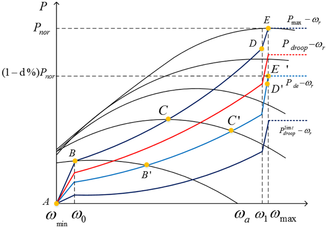
The droop power curve.

When the frequency dips, the droop curve moves toward the P_max-ω_r curve. Thus, the reference power with the same rotor speed is larger, that is, more active power from the wind turbine is delivered to the system.

The droop response is a minute-term time response. Thus, the P_max-ω_r curve is the upper limit of the droop power curve. The additional power from the P_droop-ω_r curve does not exceed the maximum available power.

When Δf_s = 0, P_droop-ω_r is the same as the de-loaded power curve. Otherwise, when the frequency rises, the power curve moves down, and the reference power with the same rotor speed changes to a smaller value. P_droop^limit-ω_r is the lower limit droop curve (as seen in Figure 5) and is near 80% of the maximum power curve.

Therefore, the droop power curve provides droop frequency support for the wind turbine, similar to the droop response in the traditional auxiliary frequency controller.

Note that there is always an intersection of the droop power curve and the captured wind power curve (equilibrium point). This means that the DFIG always converges to the equilibrium point in any case. Furthermore, the droop power curve definition does not contain any control gains in (9).

Inertia power curve

Furthermore, to provide inertia supports for the system frequency, the droop power curve, P_droop-ω_r, is further modified into an inertia power versus rotor speed curve, called P_in-ω_r, based on the ROCOF (df_s/dt).

In this paper, the inertia power curve is defined in (11) as below.

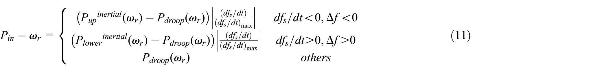
P_{in} - ω_{r} = {\begin{matrix} ({P_{up}}^{inertial} (ω_{r}) - P_{droop} (ω_{r})) | \frac{(d f_{s} / dt)}{{(d f_{s} / dt)}_{max}} | & d f_{s} / dt < 0, Δ f < 0 \\ ({P_{lower}}^{inertial} (ω_{r}) - P_{droop} (ω_{r})) | \frac{(d f_{s} / dt)}{{(d f_{s} / dt)}_{max}} | & d f_{s} / dt > 0, Δ f > 0 \\ P_{droop} (ω_{r}) & others \end{matrix}

(11)

where P_up^inertial-ω_r is the upper limit of the inertia power curve, and P_lower^inertial-ω_r is the lower limit of the inertia power curve. (df_s/dt)_max is the maximum measurement df_s/dt during the frequency event process.

To obtain (df_s/dt)_max, a latch is used to store the maximum value. This means that if a new measurement (df_s/dt) value is larger than the old storage value, the new value replaces the old storage value. Otherwise, the latch keeps the old storage value.

P _up ^inertial-ω_r is defined as in (12), which borrows from Wang and Tomsovic (2018). P_up^inertial-ω_r also shown in Figure 6.

P_{up}^{inertial} (ω_{r}) = \frac{P_{up}^{T lim} (ω_{a}) - P_{de} (ω_{0})}{ω_{a} - ω_{0}} (ω_{r} - ω_{0}) + P_{de} (ω_{0})

(12)

Figure 6.

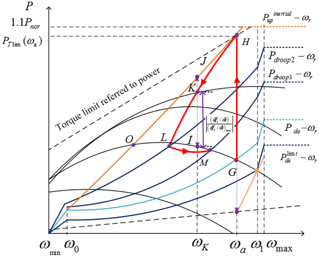
The inertia power curve.

P_Tlim is the torque limit relative to the power curve. ω_a is the initial rotor speed.

To avoid the rapid and excessive increase in the output power causing the wind turbine’s mechanical torsion, the power limit P_limit and the maximum torque limit T_g^max are often set to 1.1 pu and 1.07 pu (Yang et al., 2018a) .

The minimum torque limit T_g^min are often set to 0.05 pu (Ochoa and Martinez, 2017). The rotor speed increases during the frequency increase event. Therefore, the definition of the P_lower^inertial-ω_r is only considered the range of the rotor speed higher than the current rotor ω_a. Similarly, the definition of P_lower^inertial-ω_r is required to prevent the speed rotor over-accelerating. The P_up^inertial-ω_r is given in (13), and as the red curve shown in Figure 6.

P_{lower}^{inertial} (ω_{r}) = \frac{P_{lower}^{T lim} (ω_{a}) - k_{de}^{80 %} ω_{1}^{3}}{ω_{a} - ω_{1}} (ω_{r} - ω_{1}) + k_{de}^{80 %} ω_{1}^{3}

(13)

To explain the frequency regulation proceeding, a frequency drop event is taken as an example, and the trajectory of operating point during the frequency regulation process is depicted by the red curve in Figure 6.

At the initial time, ‘G’ is assumed to be the initial operating point located at the de-loaded curve. Δf_s and |df_s/dt| are negative values, and df_s/dt quickly drops to the minimum value. That is, |df_s/dt| reaches the maximum value. The de-loaded power curve quickly turns into the upper limit inertial curve, P_up^inertial-ω_r. Thus, the operating point switch from the ‘G’ to the point ‘H’. The wind turbine releases the maximum allowable power for the supported frequency.

Then, Δf_s and |df_s/dt| decreases. According to (9), the droop power curve moves up with Δf_s. Meanwhile, the rotor speed ω_r decreases because of the extra active power releasing. ‘J’ is the corresponding point with ω_K located at P_up^inertial-ω_r curve, while ‘I’ is the corresponding point with ω_K located at P_droop-ω_r curve. Because of the decrease of the df_s/dt (df_s/dt < (df_s/dt)_max), according to (11), the operating point moved from ‘H’ to ‘K’ (P_in(ω_K),ω_K). The additional active power from the wind turbine is gradually decreased. Along with df_s/dt approach to zero, the operating point moves from the P_up^inertial-ω_r curve to the droop power curve.

When df_s/dt = 0, the frequency reaches the lowest point. At this time, the inertia power curve turns into the droop power curve. The operating point ‘K’ will turn into ‘L’ located into the droop power curve P_droop2-ω_r.

Then, the frequency recovery starts. df_s/dt and Δf_s are opposite in sign. Unfortunately, the inertia response is not beneficial for frequency recovery. Thus, when df_s/dt > 0 and Δf_s < 0, the power curve maintains the droop power curve. The inertial power curve is only enabled when df_s < 0 and df_s/dt < 0. As the frequency recovery (Δf_s increase), the P_droop2-ω_r curve will move downward to the P_droop3-ω_r curve. As illustrated in Figure 6, the operating point will move from ‘L’ to ‘M’.

The P_up^inertial-ω_r curve and the P_m-ω_r curve always has an intersection (like ‘O’ point in Figure 6), which also is an equilibrium point. Only under the extreme situations that dfs/dt keeps the max value (df_s/dt)_max, the wind turbine will converge to this intersection. The rotor speed of this intersection still higher the minimum rotor speed limit ω_min. Practically, the dfs/dt will gradually reduce during the frequency regulation process. Hence, the rotor speed always higher than ω_min during frequency regulation process. Otherwise, the proceeding of the frequency rise event is similar. The proposed method can ensure the wind turbine operate among the safe rotor range and prevents overdeceleration.

Noticeably, there are no control gains in (9)–(11). The output power is determined by the current measurement rotor speed and the modified power curve. Thus, unlike the existing scheme’s difficulty in choosing the proper control gains, the proposed scheme does not have any control gains.

Pitch angle control

As described in the traditional FRS control (Section II. B), in the medium and high wind areas, pitch angle control is necessary to add to limit the rotor speed and help de-load control. However, in traditional control, wind speed information is required to decide the wind speed area and calculate the value of the compensation pitch β_de. However, the inaccurate wind speed measurement may be harmful to the control performance. Furthermore, a complex calculation is needed to calculate β_de. In this paper, improved pitch angle control is designed.

Figure 7 shows the de-loaded power, maximum power pitch angle β_m, de-loaded pitch angle β_de, and difference angle (between the aforementioned two angles) Δβ versus wind speed. The maximum power pitch angle remains zero until the wind speed reaches V₂. Then, the pitch angle gradually increases to reduce the capture of wind power.

Figure 7.

Pitch angle and de-loaded power at various wind speeds.

The de-loaded pitch angle remains zero until the wind speed reaches V₁. Then, the pitch angle increases to realize de-loaded control. During V₁ and V₂, which is called the medium wind speed area aforementioned, both pitch angle control and rotor speed control are used to realize de-loaded control. At wind speeds higher than V₂, only the pitch angle is used to realize de-loaded control.

Observing Δβ in Figure 7, Δβ can be divided into three segments: a low wind speed area where the wind speed lowers V₁, where it is zero; a medium wind speed area during V₁ and V₂, where it is a nonlinear curve; and a high wind speed area, higher than V₂, where it has a constant value (nearly 1.6° in this paper).

Figure 8 shows the wind power coefficient C_p versus pitch angle under different tip speed ratios.

Figure 8.

Wind power coefficient C_p versus pitch angle under different tip speed ratios.

In the vicinity of λ_opt (λ_opt = 10.5 in this paper), C_p seems not to be influenced by the different λ. Therefore, the pitch angle is an almost constant value when C_p is not a considerable reduction. This is the reason that in the high wind area, Δβ remains almost constant to realize a certain power reserve.

Linearly fitting the λ_opt curve to obtain the approximate linear relationship between C_p and pitch angle:

C_{p} = - 0.0276 β + 0.44

(14)

If the DFIG operates at a 10% power reserve, β will increase by approximately 1.6°.

Further observing Figure 7 in the low wind area, the Δβ is zero, where the de-loaded power is below 0.38 P_nor; in the medium wind speed area, where the de-loaded power is between 0.38P_nor and 0.9 P_nor, the Δβ varies with de-loaded power. At high wind speeds, where the de-loaded power remains at 0.9 P_nor, Δβ remains at a constant value of 1.6°.

The Δβ versus the de-loaded power curve is described in Figure 9 and the polynomial fitting function given in (15).

Δ β = {\begin{matrix} \begin{matrix} 0 & P_{de} < 0.38 \end{matrix} \\ \begin{matrix} 20.9 {P_{de}}^{3} - 48.17 {P_{de}}^{2} + 37.62 P_{de} - 8.42 & 0.38 \leq P_{de} < 0.9 \end{matrix} \\ \begin{matrix} 1.6 & P_{de} = 0.9 \end{matrix} \end{matrix}

(15)

According to (15), Δβ can be obtained based on the de-loaded power P_de. Wind speed information is not required.

Figure 9.

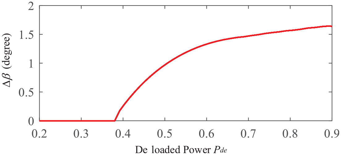
Δβ versus the de-loaded power curve.

In the medium and high wind speed areas, the pitch angle must be adjusted to release more or less active power for participation in frequency regulation. The improved pitch control diagram is given in Figure 10 below.

Figure 10.

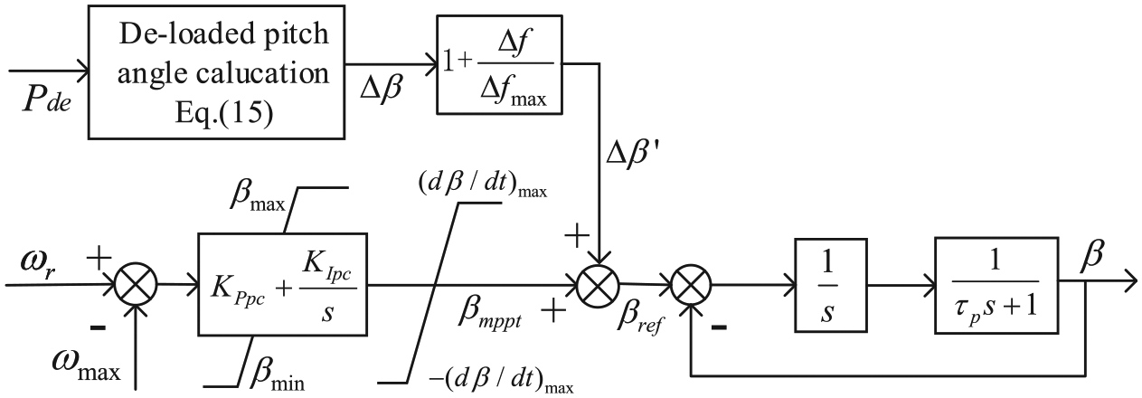
The proposed pitch angle control scheme.

As seen in Figure 10, Δβ is obtained from equation (15), and a simple linear method is used to calculate the compensation pitch angle Δβ′,

Δ β' = (1 + \frac{Δ f}{Δ f_{max}}) Δ β

(16)

Δβ′ regulate with the system frequency. When Δf = −Δf_max, Δβ′ is equal to 0, and β_ref = β_mppt. When Δf = 0, Δβ′ is equal to Δβ, and β_ref = β_de (the pitch angle in de-loaded mode).

As shown in the modified pitch angle control description in Figure 10, wind speed information is not required. The pitch angle can help the de-loaded operation and the frequency regulation of wind turbines in medium and high wind speed areas.

Case study

In this section, simulations using MATLAB/SIMULINK 2018 Student Suite Version, MathWorks, Natick, MA, USA are carried out to verify the proposed frequency regulation scheme’s efficacy.

Figure 11 shows the single bus model of the small isolated power system used in the paper. It includes static loads, one thermal plant, one hydropower plant, and one aggregated DFIG-based wind power plant. The total capacity of the power systems is 1250 MW.

Figure 11.

Single-line diagram of test power system for simulation.

Simplified governor-based models from Akbari and Madani (2014) are used to simulate thermal and hydropower plants (see Figure 12).

Figure 12.

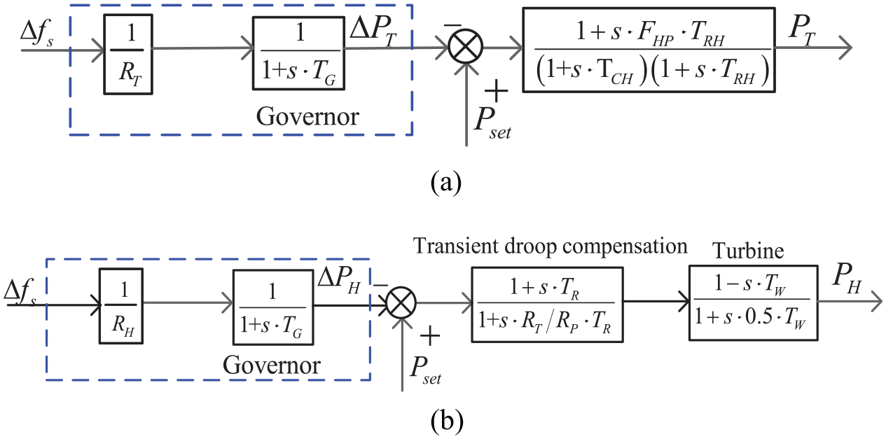
Governor-based models of conventional power plants: (a) Single-reheat steam plant (b) Hydro plant.

The droop characteristics of conventional plant speed governors have been enabled. The values of the most significant parameters are summarized in Appendix Tables A2 and A3.

To simulate the wind power plant, an equivalent generator with 100 times the nominal power of one DFIG is assumed. The parameters of DFIG-based VSWTs are given in Appendix Table A1. The performance of the proposed scheme for DFIG-based VSWTs is compared to that of MPPT, the conventional FRS with fixed gain under various wind speeds.

In traditional FRS with fixed gain, K_w is set to 30 and 15, while 1/R_w is set to 24 and 7. Under medium wind speed conditions, when a larger gain is selected, the inertial control performance of the DFIG can be effectively improved while ensuring stable operation. In comparison, a smaller gain is selected to maximize the lowest frequency point (FN) while ensuring stable operation of all DFIGs under low wind conditions. It is worth noting that the values of large gain and small gain are just an example of traditional FRS. If the system changes, these values should be changed appropriately.

Cases 1, 2, and 3 refer to the constant wind speed in the low wind speed area, the medium wind speed area and the high wind speed area, respectively. In cases 4 and 5, the wind speed is assumed to be reduced at the instant of an event, from 9 to 7.5 m/s for 10 and 1 second, respectively. Case 6 is the random wind speed in low wind area. In all cases, if the rotor speed reaches ω_min, the FRS (not including de-loaded control) are disabled by disconnecting the frequency measurement.

Compared with the decreased output power, DFIG-based VSWTs have more difficulty increasing the output power when the frequency dips. Thus, at 60 seconds, the system load suddenly increases by 0.1 pu and causes a frequency dip event for all cases.

Effects of wind speeds

Case 1: Low wind speed area

Figure 13 illustrates the results for a wind speed of 8 m/s in the low wind speed area, where the DFIG-based VSWTs only use overspeed control to realize de-loaded control. Figure 13 shows the result of Case 1.

Figure 13.

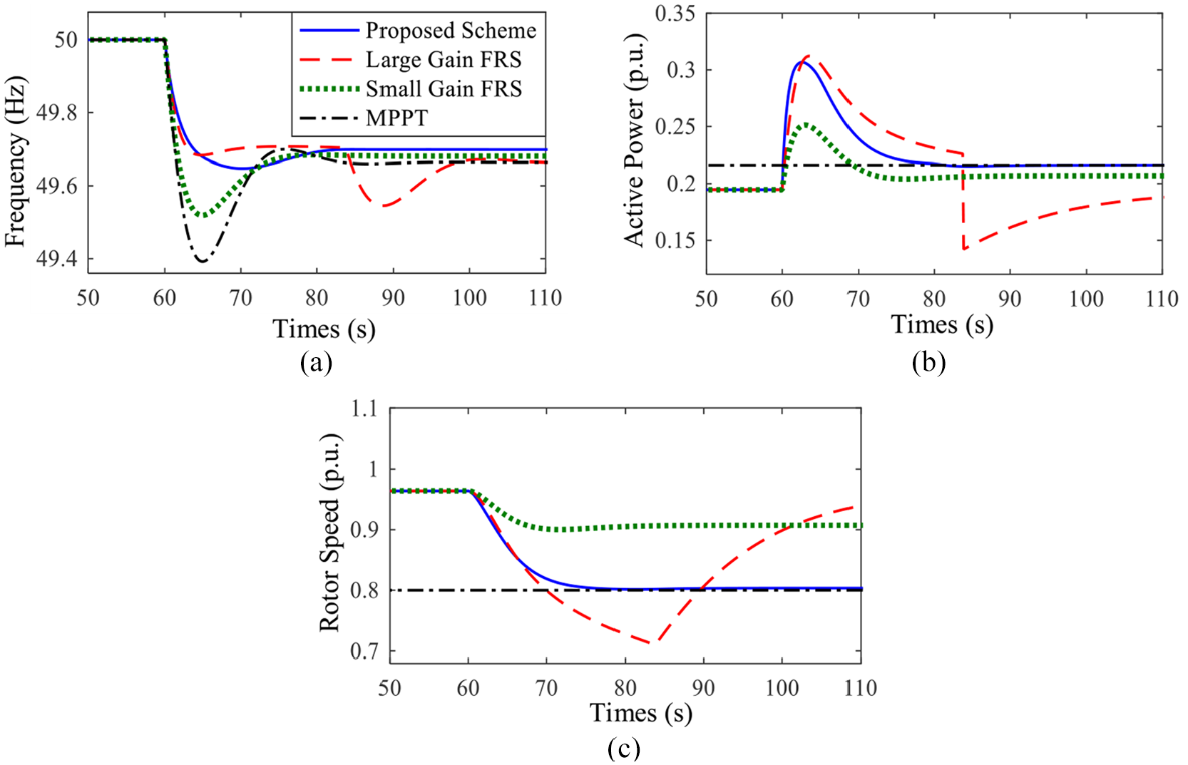
Results for Case 1: (a) system frequency, (b) active power of DFIG, and (c) rotor speed of DFIG.

Before 60 seconds, for the traditional FRS and the proposed FRS, the initial power is maintained at 0.9 P_m, which is 0.194 pu. The output power of MPPT always remains at the maximum power of 0.216 pu.

For the large gain FRS, the system frequency reduction speed is slower than that of the small gain FRS and the proposed scheme. Because the large gain FRS releases more power in the initial stage of the grid, the rotor speed decreases more. As shown in Figure 13(c), at 83.86 seconds, the speed of the DFIG reaches ω_min. To protect the wind turbine, the frequency support control is disabled and causes sudden active power drops, which result in a secondary frequency dip. The first frequency nadir (FN) is 49.68 Hz, and the second FN is 49.55 Hz.

The small gain FRS can ensure that DFIGs operate in a safe rotor speed range. However, due to the limited support it provides, its peak power is only 0.25 pu, and FN is 49.46. The steady frequency is 49.68 Hz.

For the proposed scheme, the peak power is 0.31 pu, larger than the small gain and smaller than the large gain FRS. However, it can prevent the wind turbines from excessively releasing kinetic energy through the modified power versus rotor speed curves. The rotor speed almost reaches but does not exceed ω_min. The FN is 49.65 Hz. It is 0.13 Hz higher than that for the small gains. The steady frequency is 49.7 Hz, 0.02 Hz larger than the small gain FRS.

Figure 14 illustrates the result of the operation at a wind speed of 10 m/s.

Figure 14.

Results for Case 1: (a) system frequency, (b) active power of DFIG, and (c) rotor speed of DFIG.

Due to the increase in wind speed, the traditional large-gain FRS’s rotor speed does not exceed the lower limiter. Compared with the large gain FRS, the proposed scheme shows a better performance. The reason is that the proposed FRS has a potential self-adaption. With increasing wind speed, the active power for the frequency support increases.

The FN of the small gain FRS is 49.48 Hz, the steady frequency is 49.67 Hz, the FN of the large gain FRS is 49.65 Hz, the steady frequency is 49.7 Hz, and the proposed frequency is 49.7 Hz, which is 0.05 Hz larger than that of the large-gain FRS. The steady frequency is 49.72 Hz, which is 0.02 larger than the large gain FRS.

Case 2: Medium wind speed area

Figure 15 illustrates the result of Case 2. In this case, the wind speed of the DFIG is 11 m/s in the medium wind area.

Figure 15.

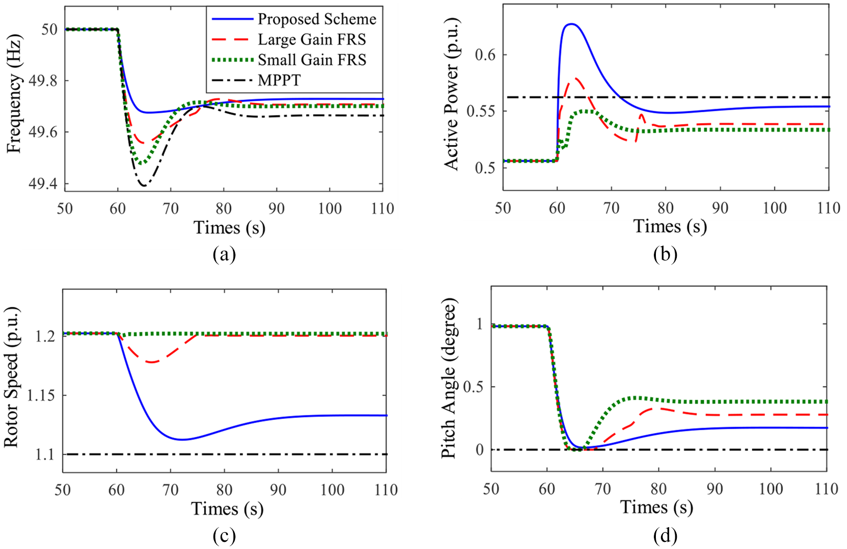
Results for Case 2: (a) system frequency, (b) active power of DFIG, (c) rotor speed of DFIG, and (d) pitch angle.

As shown in Figure 15(a), the FN of the traditional small gain FRS is 49.48 Hz, which is 0.08 Hz higher than the FN of MPPT control but 0.08 Hz lower than the FN of the large gain FRS. The proposed scheme’s FN is 49.73 Hz, which is 0.17 Hz higher than the large gain FRS. The proposed scheme’s steady frequency is 49.7 Hz, 0.03 Hz larger than the large gain FRS and 0.04 Hz larger than the small gain FRS.

In Figure 15(b), the output power of MPPT is always the maximum power of 0.5623 pu. Before 60 seconds, the traditional scheme and the proposed scheme maintain an initial power of 0.9. Initially, the proposed scheme’s additional power is greater than that of the large gain and the small gain FRS. The designed inertia power curve is used to provide inertia support. The peak power of the small gain is 0.55 pu, that of the large FRS is 0.58 pu, and that of the proposed scheme is 0.627 pu.

In Figure 15(c), the selected large- and small-gain FRSs can ensure that the DFIG works in the safe rotor speed range. The rotor speed of the proposed scheme converges to a lower value than the large gain FRS. Due to the potential self-adaption, the proposed scheme can adaptively release more KE from the DFIG.

As shown in Figure 15(d), pitch angle control is activated to provide de-loaded and frequency support control. Before 60 seconds, the DFIG runs under de-loaded mode, and the pitch angle is approximately 0.98. After 60 seconds, the pitch angle decreases to release extra power for frequency support. The proposed scheme shows a deeper pitch drop than the others. It seems that the proposed scheme can better utilize rotor speed control to provide frequency support.

Case 3: High wind speed area

Figure 16 illustrates the result of Case 3. In this case, the wind speed is 13.6 m/s in the high wind speed area.

Figure 16.

Results for Case 3: (a) system frequency, (b) active power of DFIG, (c) rotor speed of DFIG, and (d) pitch angle.

In high wind speed areas, the frequency regulation is depended on the pitch angle control. Figure 16(c) shows that the rotor speed is near 1.21 pu for all the control schemes. In Figure 16(d), the proposed scheme’s pitch angle drops deeper than that of the traditional scheme. Therefore, the output power from the wind turbine is higher than that of the large gain FRS. The FN of the proposed scheme is better than that of the large gain FRS. As shown in Figure 16(a), the FN of the small gain FRS is 49.59 Hz, which is 0.03 Hz lower than the large FRS and 0.09 Hz lower than the proposed scheme.

Because of the different drop level of the pitch angle, the proposed scheme’s steady frequency is the best, that is, 49.79, while the steady frequency of the large-gain FRS is 49.77 Hz, and that of the small-gain FRS is 49.74 Hz.

The results of the three cases clearly show that the proposed scheme can provide better frequency support than the traditional scheme for the whole wind speed range, regardless of low, medium, and high wind speeds. It has the potential to provide adaptive frequency support for different wind speeds and prevent overdeceleration of the DFIG.

Effects of varying wind speeds

This section introduces the test results under variable wind speed conditions. The wind speed decreases at different time intervals, and the actual random wind speed is considered.

Case 4: Decreasing wind speed from 9 to 7.5 m/s for 10 seconds

Figure 17 illustrates the result of Case 4, where the wind speed decreases from 9 to 7.5 m/s for 10 seconds at 60 seconds.

Figure 17.

Results for Case 4: (a) wind speed, (b) system frequency, (c) active power of DFIG, and (d) rotor speed of DFIG.

The proposed FRS prevents the rotor speed from exceeding ω_min and the rotor speed converges to 0.77 pu rapidly, which is a smaller value than the small gain FRS. Its FN is 0.02 Hz larger than the small gain and 0.18 Hz larger than the secondary frequency drop of the large gains FRS.

Case 5: Decreasing wind speed from 9 to 7.5 m/s for 1 seconds

Figure 18 shows the result of Case 5. In this case, the wind speed was reduced from 9 to 7.5 m/s at 60 seconds for 1 seconds.

Figure 18.

Results for Case 5: (a) wind speed, (b) system frequency, (c) active power of DFIG, and (d) rotor speed of DFIG.

Compared with Case 4, the wind speed reduction is faster than that in Case 4. This results in a faster reduction in the rotor speed than Case 4. Along with the wind speed reduction, the output power of the wind turbine decreases.

For the small gain FRS, the wind turbine still has stable operation, and the FN is 49.41 Hz, 0.07 Hz lower than the small gain FRS in case 4.

However, for the large gain FRS, the rotor speed reaches ω_min at 70.6 seconds, which is 2.5 seconds earlier than case 4, and it causes a secondary frequency drop to occur. The secondary FN at 74.47 seconds is 49.3 Hz.

Conversely, our proposed scheme can still successfully prevent overdeceleration even in this case by rapidly reducing the active power, as shown in Figure 18(d). The speed converges to a safe value of 0.77 pu. The FN is 0.05 Hz higher than the small gain FRS. The steady-state value of the frequency is similar to the large gain.

Case 6: Random wind speed

Figure 19 presents the simulation results of case 6. The actual measured wind speed (low wind speed area) in Northeast China. The load suddenly increases 0.1 pu at 60 seconds.

Figure 19.

Results for Case 6: (a) random wind speed, (b) system frequency, (c) active power of DFIG, and (d) rotor speed of DFIG.

For MPPT, the active power is only affected by wind speed. The wind turbine does not participate in frequency regulation. The FN is 49.38 Hz.

The stable operation of the DFIG can be ensured in small gain FRS. However, the additional active power for the frequency regulation is insufficient. The FN is 49.59 Hz, which is 0.12 Hz lower than the proposed scheme.

Due to the excessive active power released in the large gain FRS, the rotor speed drops fast and exceeds ω_min at 130 seconds, causing a secondary frequency drop. The secondary FN is 49.42 Hz, which is the lowest value in this case.

From Figure 19(b), before the FRC disabled, the large gain FRS shows a slightly better frequency response than the proposed FRS. However, it will result in an overdeceleration of the DFIG and cause a secondary frequency dip.

The simulation results of cases 4, 5, and 6 verify that even under variable wind speed conditions, the proposed scheme still prevents the wind turbine from over decelerating.

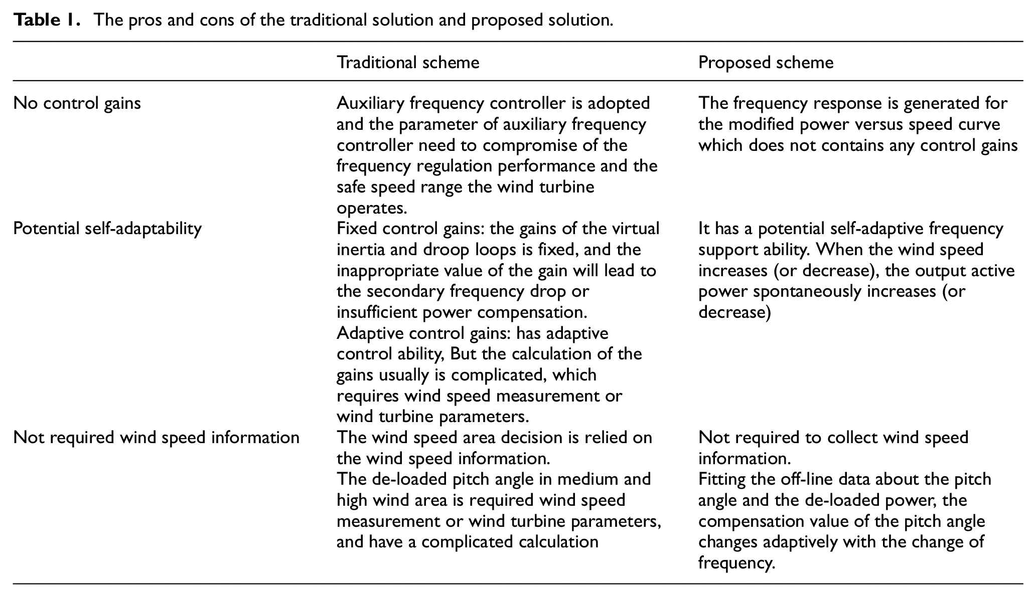
In summary, the pros and cons of traditional and proposed solution are listed in Table 1 below.

Table 1.

The pros and cons of the traditional solution and proposed solution.

	Traditional scheme	Proposed scheme
No control gains	Auxiliary frequency controller is adopted and the parameter of auxiliary frequency controller need to compromise of the frequency regulation performance and the safe speed range the wind turbine operates.	The frequency response is generated for the modified power versus speed curve which does not contains any control gains
Potential self-adaptability	Fixed control gains: the gains of the virtual inertia and droop loops is fixed, and the inappropriate value of the gain will lead to the secondary frequency drop or insufficient power compensation.	It has a potential self-adaptive frequency support ability. When the wind speed increases (or decrease), the output active power spontaneously increases (or decrease)
	Adaptive control gains: has adaptive control ability, But the calculation of the gains usually is complicated, which requires wind speed measurement or wind turbine parameters.
Not required wind speed information	The wind speed area decision is relied on the wind speed information.	Not required to collect wind speed information.
	The de-loaded pitch angle in medium and high wind area is required wind speed measurement or wind turbine parameters, and have a complicated calculation	Fitting the off-line data about the pitch angle and the de-loaded power, the compensation value of the pitch angle changes adaptively with the change of frequency.

Conclusion

With the high penetration of wind power generator, the frequency stability is still a critical issue in the power system because of the reduction of the inertia and frequency regulation capability. This paper proposes a novel frequency regulation scheme based on parameterized power curve for the de-loaded wind turbine during the whole wind speed range.

Compared with the existing scheme, the auxiliary frequency controller is replaced by a modified power versus rotor speed curve according to the frequency deviation and the rate of change of the frequency to provide both inertia and a droop frequency response. In the traditional scheme, the control gains of the auxiliary frequency controller are hard to select because of the compromising of the rotor speed safe and the frequency regulation performance. However, the proposed scheme does not contain any gains and can be applied to WTGs with different wind speeds. Further, it has a potential self-adaptability that the active power will automatically increase with wind speed increases.

An improved pitch angle control is designed which is generally adapts for the whole wind speed range without wind speed information. The curve of the de-loaded pitch angle versus de-loaded power is fitting by off-line modeling. And then, the compensation pitch angle is simply calculated by frequency measurement information, avoiding the use of wind speed information and the complicated calculation.

The comparison simulation results under low wind speed, medium wind speed, high wind speed, and variable wind speed were evaluated. The simulation results clearly show that the scheme has a better performance than the traditional frequency regulation strategies for improving the frequency response and preventing rotor speed over deceleration under variable wind conditions.

Footnotes

Appendix

Table A3.

Hydro-power plant parameters.

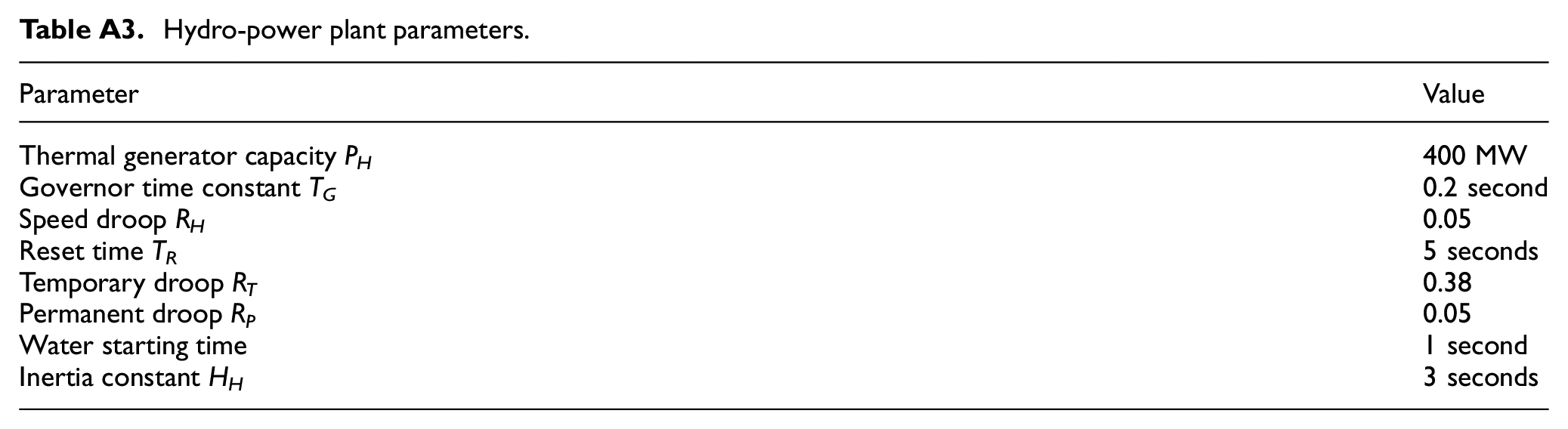
Parameter	Value
Thermal generator capacity P_H	400 MW
Governor time constant T_G	0.2 second
Speed droop R_H	0.05
Reset time T_R	5 seconds
Temporary droop R_T	0.38
Permanent droop R_P	0.05
Water starting time	1 second
Inertia constant H_H	3 seconds

Declaration of conflicting interests

The author(s) declared no potential conflicts of interest with respect to the research, authorship, and/or publication of this article.

Funding

The author(s) disclosed receipt of the following financial support for the research, authorship, and/or publication of this article: This article was funded by National Natural Science Foundation of China (Grant id 52077030, U18866601) and Jilin Province Science and technology development plan project (Grant Id 20190201289JC).

ORCID iD

Cheng Zhong

References

Aho

Buckspan

Laks

, et al. (2012) A tutorial of wind turbine control for supporting grid frequency through active power control. In: 2012 American Control Conference (ACC), Montreal, QC, 27–29 June, pp.3120–3131.

Akbari

Madani

(2014) Analytical evaluation of control strategies for participation of doubly fed induction generator-based wind farms in power system short-term frequency regulation. IET Renewable Power Generation 8(3): 324–333.

Altin

Hansen

Barlas

, et al. (2018) Optimization of short-term overproduction response of variable speed wind turbines. IEEE Transactions on Sustainable Energy 9(4): 1732–1739.

Babu

Ramesh

(2013) Wind energy conversion systems – a technical review. Journal of Engineering Science and Technology 8(4): 493–507.

Chang-Chien

Lin

Yin

(2011) Enhancing frequency response control by DFIGs in the high wind penetrated power systems. IEEE Transactions on Power Systems 26(2): 710–718.

Clark

Miller

Sanchez-Gasca

(2010) Modeling of GE Wind Turbine-Generators for Grid Studies, vol. 4. Schenectady, NY: General Electric International, Inc.

Ekanayake

Jenkins

(2004) Comparison of the response of doubly fed and fixed-speed induction generator wind turbines to changes in network frequency. IEEE Transactions on Energy Conversion 19(4): 800–802.

Gao

Yan

, et al. (2019) Comprehensive frequency regulation scheme for permanent magnet synchronous generator-based wind turbine generation system. IET Renewable Power Generation 13(2): 234–244.

Global Wind Energy Outlook (2020) [Online]. Available at: www.gwec.net (accessed 26 March, 2021).

10.

Hafiz

Abdennour

(2015) Optimal use of kinetic energy for the inertial support from variable speed wind turbines. Renewable Energy 80: 629–643.

11.

Hydro Québec (2009) Transmission provider technical requirements for the connection of power plants to the Hydro Québec transmission system. Montréal, QC [Online]. Available at: http://www.hydroquebec.com/transenergie/fr/commerce/pdf/ (accessed 20 July, 2014).

12.

Kang

Muljadi

Hur

, et al. (2016) Stable adaptive inertial control of a doubly fed induction generator. IEEE Transactions on Smart Grid 7(6): 2971–2979.

13.

Kayikçi

Milanovic

(2009) Dynamic contribution of DFIG-based wind plants to system frequency disturbances. IEEE Transactions on Power Systems 24(2): 859–867.

14.

Lee

Jang

Muljadi

, et al. (2016) Stable short-term frequency support using adaptive gains for a DFIG-based wind power plant. IEEE Transactions on Energy Conversion 31(3): 1068–1079.

15.

, et al. (2019) Strategy for wind power plant contribution to frequency control under variable wind speed. Renewable Energy 130: 1226–1236.

16.

Liserre

Cardenas

Molinas

, et al. (2011) Overview of multi-MW wind turbines and wind parks. IEEE Transactions on Industrial Electronics 58(4): 1081–1095.

17.

Liu

Pan

Quan

, et al. (2019) A variable droop frequency control strategy for wind farms that considers optimal rotor kinetic energy. IEEE Access 7: 68636–68645.

18.

Liu

You

Liu

(2017) Study of wind and PV frequency control in U.S. power grids—EI and TI case studies. IEEE Power and Energy Technology Systems Journal 4(3): 65–73.

19.

Luo

Zhang

, et al. (2019) Coordinated active power control strategy for deloaded wind turbines to improve regulation performance in AGC. IEEE Transactions on Power Systems 34(1): 98–108.

20.

Margaris

Papathanassiou

Hatziargyriou

, et al. (2012) Frequency control in autonomous power systems with high wind power penetration. IEEE Transactions on Sustainable Energy 3(2): 189–199.

21.

Min

Muljadi

Park

, et al. (2016) Dynamic droop-based inertial control of a doubly-fed induction generator. IEEE Transactions on Sustainable Energy 7(3): 924–933.

22.

Morren

Pierik

De Haan

SWH

(2006) Inertial response of variable speed wind turbines. Electric Power Systems Research 76(11): 980–987.

23.

Nordic Grid Code (Nordic Collection of Rules) (2007) Nordel [Online]. Available at: https://www.entsoe.eu/ (accessed 20 July, 2014).

24.

Ochoa

Martinez

(2017) Fast-frequency response provided by DFIG-wind turbines and its impact on the grid. IEEE Transactions on Power Systems 32(5): 4002–4011.

25.

Singh

Lentijo

Sundaram

(2019a) The impact of the converter on the reliability of a wind turbine generator. In: Proceedings of the ASME 2019 power conference, Salt Lake City, UT, 15–18 July, p.V001T06A016. ASME.

26.

Singh

Matuonto

Amos

, et al. (2019b) System of systems strand tilt analysis perspective on medium high voltage stator bar and a non-destructive testing case study. In: 2019 IEEE international systems conference (SysCon), Orlando, FL, 8–11 April, pp.1–8.

27.

Singh

Matuonto

Sundaram

(2019c) Impact of imbalanced wind turbine generator cooling on reliability. In: 2019 10th International Renewable Energy Congress (IREC), Sousse, Tunisia, 26–28 March, pp.1–6.

28.

Singh

Saleh

Amos

, et al. (2018) IC6A1A6 vs. IC3A1 squirrel cage induction generator cooling configuration challenges and advantages for wind turbine application. In: ASME 2018 power conference collocated with the ASME 2018 12th international conference on energy sustainability and the ASME 2018 nuclear forum Volume 1: fuels, combustion, and material handling; combustion turbines combined cycles; boilers and heat recovery steam generators; virtual plant and cyber-physical systems; plant development and construction; renewable energy systems. Lake Buena Vista, FL, USA. 24 -28 June 2018, p.V001T06A002. ASME.

29.

Singh

Sundaram

(2020) Manufacturing deformation impact on the performance of electrical generator for the wind turbine application. Wind Engineering. Epub ahead of print 12 November 2020. DOI: 10.1177/0309524x20968816.

30.

Singh

Sundaram

(2021) Methods to improve wind turbine generator bearing temperature imbalance for onshore wind turbines. Wind Engineering. Epub ahead of print 13 May 2021. DOI: 10.1177/0309524x211015292.

31.

Singh

Sundaram

Matuonto

(2021) A solution to reduce overheating and increase wind turbine systems availability. Wind Engineering 45(3): 491–504.

32.

Singh

Sundaram

Saleh

(2019d) Addressing reduced ingress protection class & proper filter selection for open ventilated (IC3A1) wind turbine generator. In: 2019 10th International Renewable Energy Congress (IREC), Sousse, Tunisia, 26–28 March, pp.1–5.

33.

Sun

Ali

Joos

, et al. (2019) Improved VSG control for type-IV wind turbine generator considering operation limitations. In: 2019 IEEE Energy Conversion Congress and Exposition (ECCE), Baltimore, MD, 29 September–3 October, pp.2085–2091.

34.

Tang

Yin

Shen

, et al. (2019) Active power control of wind turbine generators via coordinated rotor speed and pitch angle regulation. IEEE Transactions on Sustainable Energy 10(2): 822–832.

35.

Ullah

Thiringer

Karlsson

(2008) Temporary primary frequency control support by variable speed wind turbines—potential and applications. IEEE Transactions on Power Systems 23(2): 601–612.

36.

Wang

Tomsovic

(2018) A novel active power control framework for wind turbine generators to improve frequency response. IEEE Transactions on Power Systems 33(6): 6579–6589.

37.

Wang

, et al. (2019) Adjustable inertial response from the converter with adaptive droop control in DC grids. IEEE Transactions on Smart Grid 10(3): 3198–3209.

38.

Hsu

(2019) Inertial support from WPPs that include VSWTs – a review. The Journal of Engineering 2019: 4633–4643.

39.

Yang

W-H

Y-L

, et al. (2019) Frequency regulation at a wind farm using time-varying inertia and droop controls. IEEE Transactions on Industry Applications 55(1): 213–224.

40.

Gao

, et al. (2018) State-of-the-art review on frequency response of wind power plants in power systems. Journal of Modern Power Systems and Clean Energy 6(1): 1–16.

41.

Yang

Kang

Kim

, et al. (2018a) Stable stepwise short-term frequency support of a DFIG-based wind farm. International Transactions on Electrical Energy Systems 28(3): e2495.

42.

Yang

Kim

Kang

, et al. (2018b) Temporary frequency support of a DFIG for high wind power penetration. IEEE Transactions on Power Systems 33(3): 3428–3437.

43.

Zertek

Verbic

Pantos

(2012) A novel strategy for variable-speed wind turbines’ participation in primary frequency control. IEEE Transactions on Sustainable Energy 3(4): 791–799.

44.

Zhang

Sun

Lin

, et al. (2012) Coordinated frequency regulation by doubly fed induction generator-based wind power plants. IET Renewable Power Generation 6(1): 38–47.

45.

Zhao

(2015) Wind-solar diesel microgrid frequency adjustment technology based on variable coefficient-based virtual inertia and overspeed control coordination of doubly-fed wind turbines. Journal of Electrotechnical Engineering 30(5): 59–68. (In Chinese)

46.

Zhao

Xue

Zhang

X-P

(2020) Fast frequency support from wind turbine systems by arresting frequency nadir close to settling frequency. IEEE Open Access Journal of Power and Energy 7: 191–202.