Numerical simulation of the aerodynamic characteristics of the NACA 0018 airfoil at medium range Reynolds number

Abstract

In the present work, simulations of the flow around the NACA 0018 airfoil operating at Reynolds number 7 × 10⁵ are performed using the EasyCFD software package. The influence of the advection scheme and turbulence model on the computed lift, drag and momentum coefficients is presented and an evaluation of the obtained results is made by comparison with published experimental data. It is concluded that predictions agree very well with experimental data up to 18° angle of attack, when using the SST turbulence model with the second order advection scheme. Limitations of simulations are shown when the airfoil operates at larger angles of attack, where unsteady periodic flow is verified. The turbulence model and the advection scheme affects both lift and drag values, but to a larger extent for drag. Predictions at high angles of attack overestimate both lift and drag coefficients, but underestimate the momentum coefficient.

Keywords

Wind turbines CFD aerodynamic coefficients turbulence models airfoils

Introduction

Wind turbines rotor blades are designed to optimise the energy captured from the wind. Unlike airplane wings, blades of wind turbines often operate at large angles of attack. For horizontal axis turbines, this occurs during periods of start and stop operations. Knowledge of the behaviour of blades under stall conditions are, in this case, necessary mainly for prediction of wind loads. On the other hand, blades of vertical axis wind turbines (Darrieus type) operate in the full range of angle of attack during the turbine normal working conditions. The vast majority of airfoils aerodynamic data pertain conditions of interest for the aviation industry, namely high Reynolds (Re) number and low incidence angles. Selig et al. (1995) provide aerodynamic data for several airfoil shapes, at low Reynolds numbers typical of wind turbines, but these data are for an angle of attack limited range −10 < α < 25° since, indeed, these data were obtained for low-speed aeronautics purposes. It is well known that experimental data for high incidence depends considerably on the wind tunnels configuration. While closed section wind tunnel data tends to overestimate lift and drag, open sections tend to underestimate these values, when compared with a situation where no blockage and boundary effects are present. The difficulty of such measurements is evidenced by Du et al. (2014), who present measurements of lift and drag for three different wind tunnels: open-jet and closed-jet in a 0.5 m Plint wind tunnel, and an open jet tunnel with 1.2×1.8 m cross section. These authors identified a second stall at around α = 40° and at α = 140° for a NACA 0018 airfoil at Reynolds number 1.2×10⁵. This behaviour, nevertheless, was not observed by Sheldahl and Klimas (1981), in their measurements for seven airfoils, including the NACA 0018, at similar Reynolds number conditions. At small Reynolds numbers, there is a considerable dependence of lift and drag on the Reynolds number. Timmer (2010) report, amongst other results, a summary of C_L coefficient over a 90°α range for the NACA 0012 airfoil, from measurements made by several authors in the range 5×10⁵ and 7.6×10⁵. Discrepancies between results are high and may not be completely attributed to Reynolds number dependency. Aerodynamic and aeroelastic properties of airfoils are addressed by Bai et al. (2012), who proposed a CFD method based on block iterative coupling for fluid-structure interaction. The method is applied to the NACA 0012 airfoil at Reynolds number 5×10⁶ to compute forces coefficients and flutter derivatives up to 20° angle of attack. Michna et al. (2021) computed the transitional flow over the DU 91-W2-250 airfoil for Reynolds numbers in the range 3×10⁶– 6×10⁶, using three commercial codes. These authors report better results for C_D and C_L when using the transition SST model, compared with the fully turbulent models, but predictions fail when approaching the region of non-linear variation of C_D and C_L with the angle of attack.

Probably the first results for the NACA 0018 airfoil at low to medium Reynolds number are those by Jacobs and Sherman (1937). As pointed out by Timmer (2008), these results were affected by the too high turbulence levels of the wind tunnel, leading to an effective Reynolds number higher than the one reported. Sheldahl and Klimas (1981) published a database for seven symmetrical airfoils for a wide range of angles of attack and Reynolds number, including the NACA 0018 airfoil. These data, however, differ to some extent from the more recent measurements performed by Timmer (2008), where a correction for the influence of the wind tunnel walls was applied.

Although measurement of airfoil aerodynamic characteristics in the deep stall region represents a considerable challenge, numerical simulation is not a less difficult task. Under deep stall, the flow is completely separated and unsteady, with alternate vortex shedding associated with fluctuations in both lift and drag, thus representing a major challenge for turbulence modelling. This is probably one of the reasons why, in the author’s knowledge, no data is available in the literature in what concerns CFD simulation of highly stalled airfoils in the Reynolds number range for the small wind turbines. Published works, such as, for example, Castiñeira-Martínez et al. (2014), Hasanuzzaman and Mashud (2013), Karna (2014), Hassan et al. (2014), deal only with low incidence angles, with attached or moderately separated flow. It is shown that predictions are relatively good up to the onset of separation, but the solution rapidly degrades with increasing angle of attack after stall, when compared with experimental results.

Simulation at low Reynolds number also constitutes a challenge. Below Reynolds number 3 × 10⁵, the laminar boundary layer in the upper surface of the airfoils separates even at low angles of attack, with a strong influence on the remaining flow field. If transition to turbulence occurs, flow reattachment takes place, with a strong influence on the aerodynamic coefficients. The ability of turbulence models to correctly model laminar to turbulence transition is thus of utmost importance to correctly simulate the aerodynamic behaviour of airfoils at very low Reynolds number. Rogowski et al. (2021) demonstrated that such simulation must be carried out in transient mode and obtained a good agreement with experimental data for the NACA 0018 airfoil up to 6° angle of attack, using the transition SST turbulence model. For larger angles of attach, results degraded in comparison with experimental data, in particular for the lift coefficient.

The rotor blades of small wind turbines typically operate on the Reynolds number range 5 × 10⁴– 7 × 10⁵. The present work intends to bring more insight into the application of numerical methods for the calculation of the aerodynamic characteristics of airfoils for small wind turbines operating at Reynolds number 7 × 10⁵, in particular in what concerns the usage of non-transition turbulence models, such as the k-ω SST and the k-ε turbulence models used in the present work. Besides the influence of the turbulence model, the role that the numerical advection scheme plays on the solution is also analysed. The 2D software package EasyCFD (Lopes, 2016) is used throughout this work.

Physical and numerical model

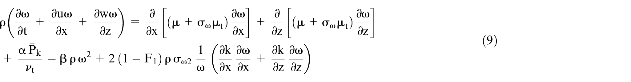
Momentum and continuity equations

The Navier-Stokes equations, describing momentum conservation, are taken in their incompressible, transient, 2D form, as:

ρ (\frac{\partial u}{\partial t} + \frac{\partial u^{2}}{\partial x} + \frac{\partial uw}{\partial z}) = \frac{\partial}{\partial x} [Γ (2 \frac{\partial u}{\partial x})] + \frac{\partial}{\partial z} [Γ (\frac{\partial u}{\partial z} + \frac{\partial w}{\partial x})] - \frac{\partial p}{\partial x}

(1)

ρ (\frac{\partial w}{\partial t} + \frac{\partial uw}{\partial x} + \frac{\partial w^{2}}{\partial z}) = \frac{\partial}{\partial z} [Γ (2 \frac{\partial w}{\partial z})] + \frac{\partial}{\partial x} [Γ (\frac{\partial u}{\partial z} + \frac{\partial w}{\partial x})] - \frac{\partial p}{\partial z}

(2)

where u and w are the Cartesian velocity components along the coordinate axis x and z, respectively, ρ is density, p is pressure and $Γ = μ + μ_{t}$ is the total viscosity, obtained as the sum of the laminar and turbulent viscosities, $μ$ and $μ_{t}$ , respectively.

The mass conservation equation is written as:

\frac{\partial u}{\partial x} + \frac{\partial w}{\partial z} = 0

(3)

The turbulent viscosity is solved with the turbulence model. The k-ε and the SST models, to be described next, are adopted in this study.

The k-ε turbulence model

The turbulence kinetic energy, k, and its dissipation rate, ε, are computed with the following transport equations (Launder and Spalding, 1972):

ρ (\frac{\partial k}{\partial t} + \frac{\partial uk}{\partial x} + \frac{\partial wk}{\partial z}) = \frac{\partial}{\partial x} [(μ + \frac{μ_{t}}{σ_{k}}) \frac{\partial k}{\partial x}] + \frac{\partial}{\partial z} [(μ + \frac{μ_{t}}{σ_{k}}) \frac{\partial k}{\partial z}] + P_{k} - ρ ε

(4)

ρ (\frac{\partial ε}{\partial t} + \frac{\partial u ε}{\partial x} + \frac{\partial w ε}{\partial z}) = \frac{\partial}{\partial x} [(μ + \frac{μ_{t}}{σ_{ε}}) \frac{\partial ε}{\partial x}] + \frac{\partial}{\partial z} [(μ + \frac{μ_{t}}{σ ε}) \frac{\partial ε}{\partial z}] + \frac{ε}{k} (C_{1} P_{k} - C_{2} ρ ε)

(5)

where P_k is the production rate of k as the results of the velocity gradients:

P_{k} = μ_{t} [2 {(\frac{\partial u}{\partial x})}^{2} + 2 {(\frac{\partial w}{\partial z})}^{2} + {(\frac{\partial u}{\partial z} + \frac{\partial w}{\partial x})}^{2}]

(6)

The turbulent viscosity is $μ_{t} = C_{μ} \frac{ρ k^{2}}{ε}$ and the remaining model constants are:

C_{μ} = 0.09 σ_{k} = 1.0 σ_{ε} = 1.3 C_{1} = 1.44 C_{2} = 1.92

(7)

The k-ω SST turbulence model

The SST model (Menter, 1993) blends the k-ε and the k-ω models, taking benefit of the advantages of each of these models. The k-ω model is more accurate near the wall but presents a high sensitivity to the ω values in the free stream region, where the k-ε model shows a better behaviour. The blending function is a weighting factor based on the nearest wall distance. The governing equations are:

ρ (\frac{\partial k}{\partial t} + \frac{\partial u k}{\partial x} + \frac{\partial w k}{\partial z}) = \bar{P_{k}} - β * ρ ω k + \frac{\partial}{\partial x} [(μ + σ_{k} μ_{t}) \frac{\partial k}{\partial x}] + \frac{\partial}{\partial z} [(μ + σ_{k} μ_{t}) \frac{\partial k}{\partial z}]

(8)

\begin{matrix} ρ (\frac{\partial ω}{\partial t} + \frac{\partial u ω}{\partial x} + \frac{\partial w ω}{\partial z}) = \frac{\partial}{\partial x} [(μ + σ_{ω} μ_{t}) \frac{\partial ω}{\partial x}] + \frac{\partial}{\partial z} [(μ + σ_{ω} μ_{t}) \frac{\partial ω}{\partial z}] \\ + \frac{α {\bar{P}}_{k}}{ν_{t}} - β ρ ω^{2} + 2 (1 - F_{1}) ρ σ_{ω 2} \frac{1}{ω} (\frac{\partial k}{\partial x} \frac{\partial ω}{\partial x} + \frac{\partial k}{\partial z} \frac{\partial ω}{\partial z}) \end{matrix}

(9)

where ω is the frequency of dissipation of turbulent kinetic energy (s⁻¹). The production of turbulent kinetic energy is limited to prevent the build-up of turbulence in stagnant regions:

\bar{P_{k}} = min (P_{k}, 10 β * ρ k ω)

(10)

The weighting function F₁ is given by:

F_{1} = \tanh {{min [max (\frac{\sqrt{k}}{β * ω y}; \frac{500 ν}{y^{2} ω}); \frac{4 ρ σ_{ω 2} k}{C D_{k ω} y^{2}}]}^{4}}

(11)

C D_{k ω} = max (2 ρ σ_{ω 2} \frac{1}{ω} \frac{\partial k}{\partial x_{j}} \frac{\partial ω}{\partial x_{j}}, 10^{- 10})

(12)

where y represents the distance to the nearest wall and $ν$ is the laminar dynamic viscosity. F₁ is zero away from the wall (k-ε model) and changes to unit inside the boundary layer (k-ω model). The turbulent viscosity is given by:

ν_{t} = \frac{a_{1} k}{max (a_{1} ω; S F_{2})}

(13)

where S represents the invariant measure of the strain rate:

S = \sqrt{S_{ij} S_{ij}}; S_{ij} = \frac{1}{2} (\frac{\partial u_{i}}{\partial x_{j}} + \frac{\partial u_{j}}{\partial x_{i}})

(14)

F_{2} = \tanh {{[max (\frac{2 \sqrt{k}}{β * ω y}; \frac{500 ρ}{μ y^{2} ω})]}^{2}}

(15)

The constants are computed as a blend of the k-ω and the k-ε models, through the following generic equation: $α = F_{1} α_{1} + (1 - F_{1}) α_{2}$ .

The constants are

\begin{matrix} α_{1} = 5 / 9 β_{1} = 3 / 40 σ_{k 1} = 0.85 σ_{ω 1} = 0.5 α_{2} = 0.44 \\ β_{2} = 0.0828 σ_{k 2} = 1 σ_{ω 2} = 0.856 β * = 0.09 \end{matrix}

(16)

The numerical method

The software package EasyCFD employs a non-structured 2D-quadrilateral mesh structure, with variables collocated at the control volume centre. The Rhie-Chow interpolation procedure (Rhie and Chow, 1983), with the modifications proposed by Majumdar (1988), is implemented in order to cope with the calculation of mass fluxes at the control volume faces. The SIMPLEC algorithm (Van Doormaal and Raithby, 1984) is adopted for the segregated solution of the primitive Cartesian velocity components and pressure. The pressure-correction equation is solved with the additive correction strategy, in a three-level multigrid (Hutchinson and Raithby, 1986). The advection scheme is responsible for the calculation of cell face values from the available information in the neighbour control volume centres. Amongst several available schemes, it is recognised that first-order schemes, such as upwind or hybrid, should be avoided, due to the inherent numerical diffusion. Second- and third-order schemes reduce numerical diffusion but may be prone to oscillations leading to over- and undershoots in the solution. This is particularly problematic for turbulent quantities, since unrealistic negative values may arise. In the present computations, the hybrid and the second-order upwind (2UpW) schemes were adopted for the solution of the momentum equations. For turbulence quantities, the hybrid scheme was used. As convergence criterion, the threshold for the normalised residuals was set to 10⁻⁸. This led to iterations number range between approximately 1500 and 2000, depending on the angle of attack, when running in steady state mode.

Domain, boundary conditions and mesh

In order to minimise boundary effects, a quite large domain around the airfoil was employed, with dimensions as shown in Figure 1, for an airfoil cord length c of 1 m. At the inlet boundary, a wind speed of 10.7 m/s was assigned, with 0.1% of turbulence intensity. Due to the distance between the inlet boundary and the airfoil, turbulence decays, starting at the inlet and reaching a minimum value of 0.08% two cord lengths from the leading edge. Lateral boundaries have a free slip condition and a parabolic condition is assigned to the outlet boundary. In order to optimise mesh nodes distributions, three mesh refinement regions, A, B and C, were adopted, as identified in Figure 1.

Figure 1.

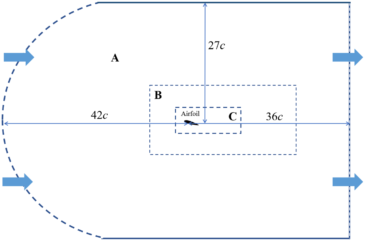
The calculation domain. Airfoil cord length is c = 1 m.

Mesh dependency tests were carried out to optimise the mesh resolution, trying to keep computational times as low as possible. Five meshes where obtained by rescaling the mesh elements size in each mesh region, leading to 73,000 nodes for the coarsest mesh and 430,000 nodes for the finest mesh. Mesh tests were performed for angle of attack α = 12°, using the SST turbulence model with the second order upwind differencing scheme. Simulation results for the lift and drag coefficients using these five meshes are presented in Figure 2. Attending to the small percentage difference in these coefficients obtained with the two finest meshes, 0.28% and 0.93% respectively, the second finest mesh, with 261,000 nodes was adopted for the present simulations. This mesh was generated using maximum target element sizes of 0.32, 0.12 and 0.02 m in mesh regions A, B and C, respectively. The airfoil was discretised with nodes spacing 0.7 mm. The distance of the first control volume node to the airfoil surface is 0.06 mm, leading to a maximum y⁺ value at the airfoil surface of 4, with average value around 1. The obtained mesh is depicted in Figure 3, where a visualisation detail around the airfoil is also included.

Figure 2.

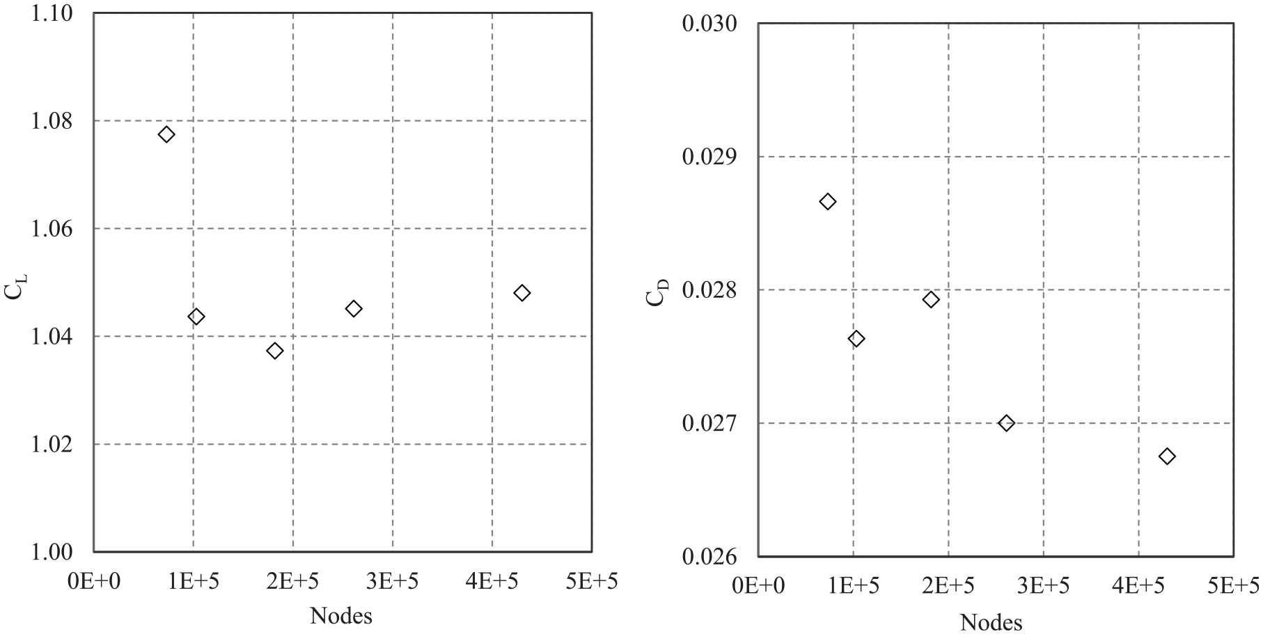
Dependence of lift and drag coefficients on mesh size, for α = 12°.

Figure 3.

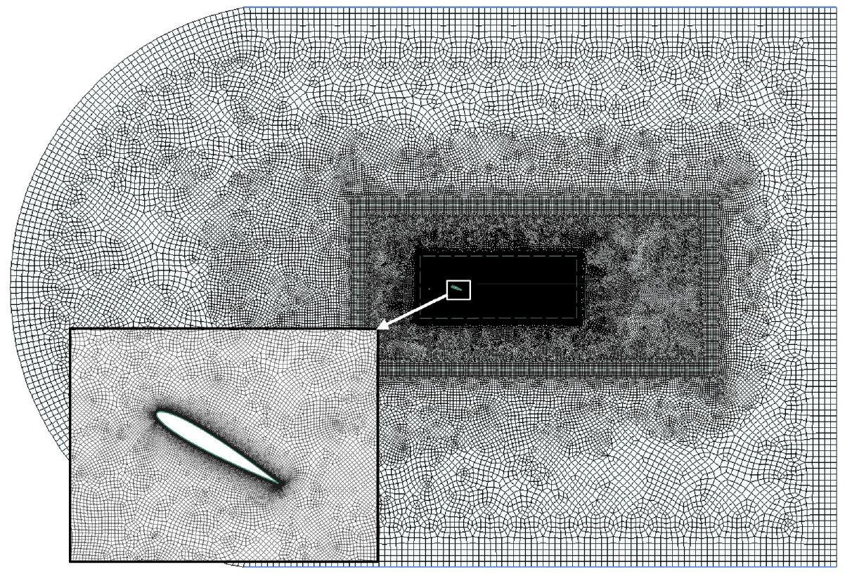
The adopted mesh for the simulations and mesh detail around the airfoil.

Simulations results

Dependence on turbulence models and advection schemes for α range 0°–18°

The first set of results are for angles of attack up to 17°, evaluating the effect for the turbulence model and the advection scheme. Data reported in Timmer (2008) include results for the untripped boundary layer, where the appearance of laminar separation is reported at α=8°, and also results for forced transition triggered with zigzag tape. Since the two turbulence models adopted in the present work do not account for transition, results will be compared only with the forced transition experimental data. Figure 4(a) depicts the lift coefficient as function of the angle of attack for present simulations, along with experimental data by Timmer (2008).

Figure 4.

(a) Lift coefficient versus of the angle of attack and (b) separation point versus angle of attack.

For the sake of completeness, non-tripped data, for which laminar separation is present, are also included. Despite all models being able to capture the general trend, the SST turbulence model coupled with the second order upwind advection scheme (2UpW) shows a marked better agreement with experimental results. The k-ε turbulence model underpredicts the lift coefficient, C_L, for most of the α range, although with a slight overprediction for 16° and 17°.

The role of the advection scheme was evaluated using the SST turbulence model. The hybrid and the 2UpW advection schemes, both with the SST turbulence model, have similar performance up to 9°. For larger α values, the hybrid scheme performance degrades, with a considerable overprediction of the lift coefficient. The bifurcation in the experimental results, visible for α > 14°, is due to a hysteresis phenomenon, as reported by Timmer (2008). According to the SST results, flow separation does not take place up to 8°. At 8°, the separation starts near the trailing edge, moving then upstream with the increase of α, as shown in Figure 4b, where the separation point distance to the leading edge, L_s, is normalised by the airfoil cord c. Separation predicted by the k-ε model starts only at 13°, and occurs farther towards the trailing edge.

Maximum lift is correctly predicted by the 2UpW_SST simulation at 15°, as seen in Figure 4(a). Then, a sudden lift loss takes place as the result of the appearance of a secondary recirculation bubble near the trailing edge, as depicted in Figure 5, where the flow visualisation is performed for α = 18°. This secondary bubble causes unsteady flow behaviour at larger angles. As will be seen for larger α, when the flow becomes unsteady, the growth of the secondary recirculation bubble is responsible for a marked decrease in lift.

Figure 5.

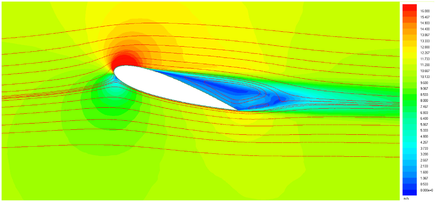
Flow streamlines (α = 18°) with 2UpW_SST configuration. Colour contours are for velocity magnitude. The presence of the secondary recirculation bubble is visible near the trailing edge.

Results pertaining the drag coefficient, C_D, are show in Figure 6(a). As for C_L, the bifurcation in the C_D experimental results, visible for α > 14°, is due to a hysteresis phenomenon, as reported by Timmer (2008). Differences between the three tested numerical configurations are now more pronounced. As for lift, the SST turbulence model with the 2UpW scheme shows the best agreement with the experiments, but with a consistent slight overprediction up to 13°, followed by a slight underprediction. Results for the k-ε turbulence model and also for the SST model with the hybrid scheme are much worst, with large C_D overpredictions over the entire α range. Figure 6b represents C_L versus C_D, synthesising thus in a different representation the information presented in Figures 4(a) and 6(a).

Figure 6.

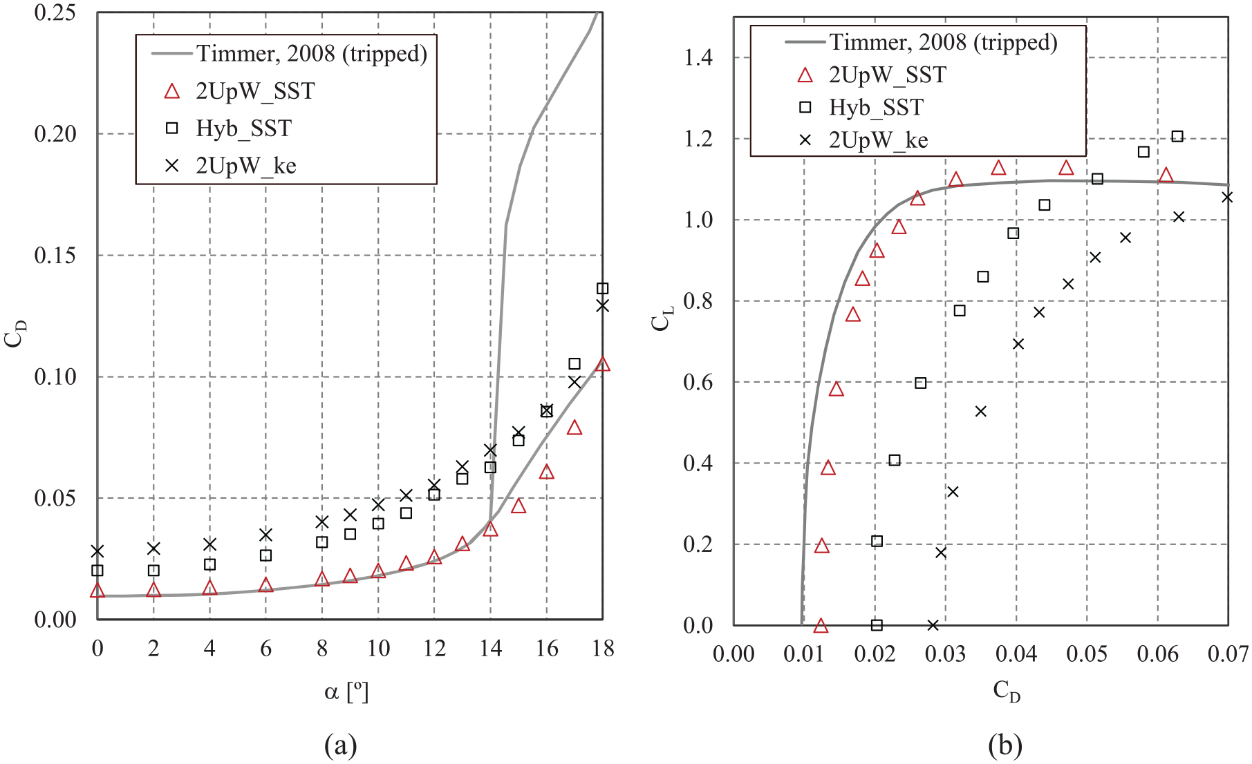
(a) Drag coefficient versus angle of attack and (b) lift coefficient versus drag coefficient.

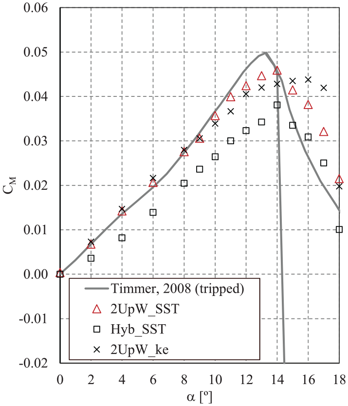
Figure 7 displays the 1/4 cord moment coefficient (C_M) values, obtained with the tested numerical configurations. The general trend is for an underprediction up to 14°, followed by overprediction for larger angles. As for C_L and C_D, results from the SST model with the 2UpW scheme show the best fitting with the experimental data.

Figure 7.

Moment coefficient versus angle of attack.

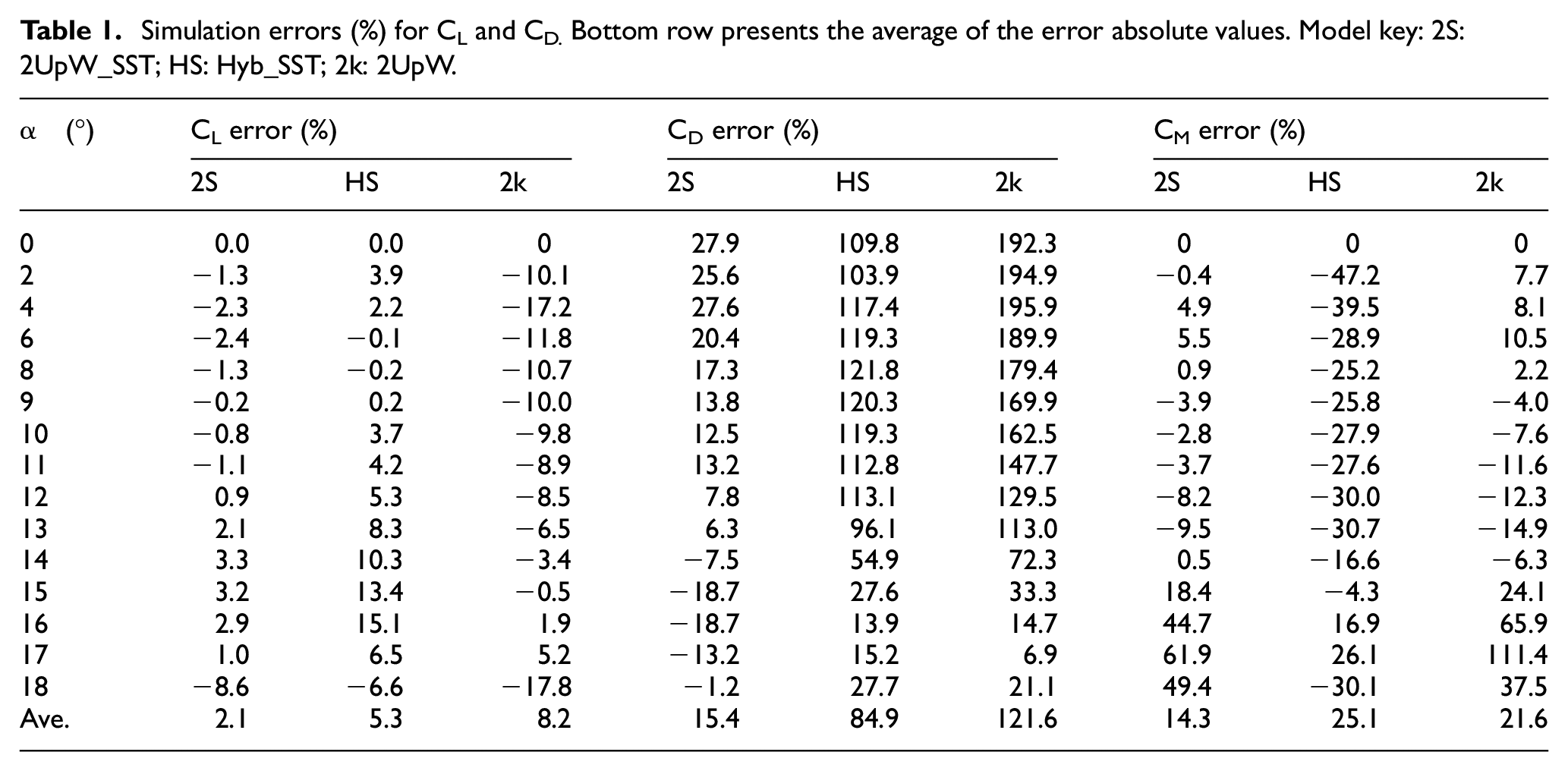
Simulation errors are defined as the percentage difference between numerical and experimental results, normalised by experimental results. Table 1 summarises simulation percentage errors for C_L, C_D and C_M using the different numerical approaches. The bottom row shows the average of the absolute value of errors.

Table 1.

Simulation errors (%) for C_L and C_D. Bottom row presents the average of the error absolute values. Model key: 2S: 2UpW_SST; HS: Hyb_SST; 2k: 2UpW.

α (°)	C_L error (%)			C_D error (%)			C_M error (%)
	2S	HS	2k	2S	HS	2k	2S	HS	2k
0	0.0	0.0	0	27.9	109.8	192.3	0	0	0
2	−1.3	3.9	−10.1	25.6	103.9	194.9	−0.4	−47.2	7.7
4	−2.3	2.2	−17.2	27.6	117.4	195.9	4.9	−39.5	8.1
6	−2.4	−0.1	−11.8	20.4	119.3	189.9	5.5	−28.9	10.5
8	−1.3	−0.2	−10.7	17.3	121.8	179.4	0.9	−25.2	2.2
9	−0.2	0.2	−10.0	13.8	120.3	169.9	−3.9	−25.8	−4.0
10	−0.8	3.7	−9.8	12.5	119.3	162.5	−2.8	−27.9	−7.6
11	−1.1	4.2	−8.9	13.2	112.8	147.7	−3.7	−27.6	−11.6
12	0.9	5.3	−8.5	7.8	113.1	129.5	−8.2	−30.0	−12.3
13	2.1	8.3	−6.5	6.3	96.1	113.0	−9.5	−30.7	−14.9
14	3.3	10.3	−3.4	−7.5	54.9	72.3	0.5	−16.6	−6.3
15	3.2	13.4	−0.5	−18.7	27.6	33.3	18.4	−4.3	24.1
16	2.9	15.1	1.9	−18.7	13.9	14.7	44.7	16.9	65.9
17	1.0	6.5	5.2	−13.2	15.2	6.9	61.9	26.1	111.4
18	−8.6	−6.6	−17.8	−1.2	27.7	21.1	49.4	−30.1	37.5
Ave.	2.1	5.3	8.2	15.4	84.9	121.6	14.3	25.1	21.6

Numerical simulations in the 0°–30° range

Tests reported in the previous sections have shown that the numerical approach consisting in the SST turbulence model coupled with the second order upwind scheme provides a good level of accuracy up to 17° of angle of attack. For larger α values, the flow becomes predominantly separated. Hysteresis in the α range 15°–24° is reported by Timmer (2008), showing a bifurcation in the aerodynamic coefficients. Simulations for α up to 30° were made in the present work. For α larger than 22°, simulations revealed flow unsteadiness, obliging the calculations to be performed in transient mode. For the transient approach, tests have shown that a time step ensuring a RMS Courant number of 1 was enough to ensure time step independency, corresponding to a real time step of 0.00015 seconds. Four iterations per time step were necessary to keep the normalised residuals below 10⁻⁸. Simulations in transient mode were carried out for a time length necessary for obtaining developed conditions in what concerns the repetition of the oscillatory pattern for the aerodynamic coefficients. Figure 8 illustrates the time evolution of C_L and C_D for the α = 30° case, showing that developed conditions were achieved after approximately 4.5 seconds of simulation. The forces oscillating behaviour is due to the formation and shedding of a counter-clockwise rotating recirculation bubble located at the trailing edge.

Figure 8.

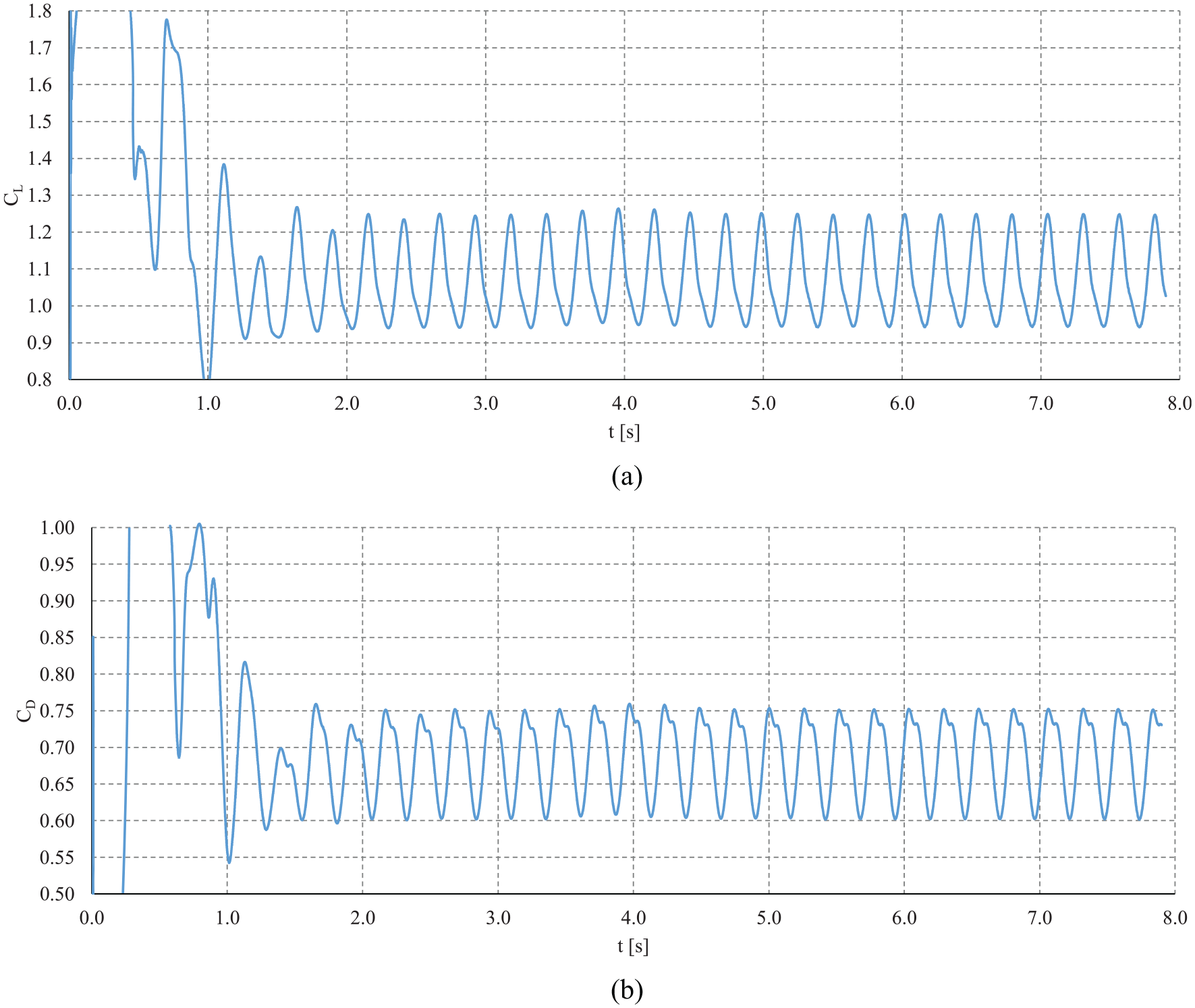
Evolution of C_L (a) and C_D (b) with simulation time, for α = 30°.

Figure 9 shows the flow visualisation at selected instants of the oscillating cycle. The small graph near each picture represents the stage in the cycle for C_L. Streamlines are selected for a better visualisation. Forces are maximum when a single clockwise vortex is present. A small counter-clockwise vortex is then formed (Figure 9(b)) at the trailing edge. This is a fast rotating vortex that feeds on the kinetic energy of the main vortex, reducing its speed and correspondingly increasing its pressure, leading to a net pressure force decrease. After reaching its maximum size (Figure 9(c)), the secondary vortex is released (Figure 9(f)), allowing the main vortex to increase its kinetic energy, with corresponding decrease in pressure.

Figure 9.

Flow streamlines pattern for α = 30°. Each frame (a) to (h) represents an instant in the oscillating cycle. Colour contours for flow velocity magnitude are according to the scale presented in Fig. 5.

The C_L and C_D values obtained by simulation using the 2UpW_SST numerical configuration for α values in the range 0°–30° are presented in Figure 10. One may observe that both C_L and C_D values agreement with experimental data deteriorate in the bifurcation region, but a good agreement recovery is obtained at α = 24°. For α > 24°, the overprediction of both C_L and C_D increases, leading to worse agreement with experimental results. It is anticipated, by the trend of both C_L and C_D, that the numerical solution continues to deteriorate as compared with experimental results for α > 30°, thus confirming the limitations of the RANS approach when dealing with largely separated flows. The oscillation amplitude is represented by the vertical bars, showing increased amplitude values with the angle of attack. The corresponding graphic for the momentum coefficient is displayed in Figure 11. The overall fitting to experimental data may be considered to be quite good, following the largest values in the bifurcation region. For 30° of angle of attack the fitting deteriorates drastically, with a considerable underprediction of C_M.

Figure 10.

Simulation results for: (a) lift coefficient and (b) drag coefficient. Vertical bars represent the oscillation range due to transient behaviour.

Figure 11.

Simulation results for the moment coefficient. Vertical bars represent the oscillation range due to transient behaviour.

Numerical simulation errors when compared with experimental data in the α range 24°–30°, as well as the oscillation amplitude and oscillation period, are listed in Table 2, showing that, with increasing angle, both the oscillation amplitude and the oscillation period increase.

Table 2.

Simulation errors (%) and oscillation data for C_L, C_D and C_M.

α (°)	C_L		C_D		C_M		Oscillation period(seconds)
	Error (%)	Oscillationamplitude	Error (%)	Oscillationamplitude	Error (%)	Oscillationamplitude
24	7.0	0.0698	1.1	0.0114	−3.5	0.0114	0.2018
26	14.1	0.1532	9.0	0.0510	11.1	0.0323	0.2280
28	14.1	0.2280	11.4	0.0991	7.5	0.0615	0.2519
30	19.5	0.3097	17.5	0.1522	31.4	0.0900	0.2570
Ave.	13.7	–	9.8	–	13.4		–

Conclusion

Numerical simulations were performed for the flow around the NACA 0018 at Reynolds number 7 × 10⁵ and inlet turbulence intensity of 0.1%. The objective was to assess the performance of the turbulence models k-ε and k-ω SST, as well as the influence of the hybrid and second order upwind advection schemes, when comparing computed results with reference wind tunnel data. Results for angle of attack in the range 0°–18° allowed to draw the following conclusions:

The influence of the advection scheme on the C_L coefficient is not significant up to α = 9°, for the SST turbulence model.

For α > 10°, the hybrid scheme with the SST turbulence model considerably overpredicts C_L.

The k-ε turbulence model considerably underpredicts the lift coefficient, C_L, for most of the α range.

The STT turbulence model with the second-order upwind scheme shows a very good performance, with a C_L average error of 2.1% over the 0°–18°α range.

Differences between the tested numerical configurations are more pronounced for C_D than for C_L, with considerable overpredictions for the k-ε turbulence model and also for the SST model with the hybrid scheme.

The STT turbulence model with the second-order upwind scheme features a C_D average error of 15.4% over the 0°–18°α range. This numerical configuration overpredicts C_D up to 13° and underpredicts C_D from 14° to 18°.

The STT turbulence model with the second-order upwind scheme provides the best results for C_M. The tested models underpredict C_M up to 14°–15° and overpredict C_M for larger angles.

Results for angle of attack in the separation region allowed to draw the following conclusions:

Simulations show an abrupt variation of the aerodynamic coefficients between 18° and 22°.

For α > 22° the solution is unsteady. As α increases, the aerodynamic coefficients oscillation period and amplitude increase, along with increasing mismatch with experimental data.

At α = 30°, the largest tested angle of attack, error values are 19.5% for C_L, 17.5% for C_D and 13.4% for C_M.

Footnotes

Acknowledgements

The authors acknowledge Ir. W.A. Timmer, Faculty of Aerospace Engineering of Delft University of Technology, The Netherlands, for kindly supplying the experimental data used in this work.

Declaration of conflicting interests

The author(s) declared no potential conflicts of interest with respect to the research, authorship, and/or publication of this article.

Funding

The author(s) received no financial support for the research, authorship, and/or publication of this article.

ORCID iD

António Manuel Gameiro Lopes

References

Bai

Sun

Lin

, et al. (2012) Numerical aerodynamic simulations of a NACA airfoil using CFD with block-iterative coupling and turbulence modelling. International Journal of Computational Fluid Dynamics 26(2): 119–132.

Castiñeira-Martínez

Solís-Gallego

González

, et al. (2014) Application of computational fluid dynamics models to aerodynamic design and optimization of wind turbine airfoils. In: International conference on renewable energies and power quality (ICREPQ’14), Cordoba, Spain, 8–10 April.

Berson

Dominy

, et al. (2014) NACA0018 behaviour at high angles of attack and at Reynolds numbers appropriate for small wind turbines. ECS technical report 2014/08, Durham University.

Hasanuzzaman

Mashud

(2013) Effect of Reynolds number on aerodynamic characteristics of an airfoil with flap. Annals of Pure and Applied Mathematics 3(1): 27–40.

Hassan

Youssef

(2014) Numerical investigation of medium range re number aerodynamics characteristics for NACA0018 airfoil. CFD Letters 6: 175–187.

Hutchinson

Raithby

(1986) A multigrid method based on the additive correction strategy. Numerical Heat Transfer 9: 511–537.

Jacobs

Sherman

(1937) Airfoil section characteristics as affected by variations of the Reynolds Number. NACA Report 586: 227–267.

Karna

Saumil

Utsav

, et al. (2014) CFD Analysis of an Aerofoil. International Journal of Engineering Research. 3(3): 154–158.

Launder

Spalding

(1972) Mathematical Models of Turbulence. London; New York, NY: Academic Press.

10.

Lopes

AMG

(2016) A numerical procedure for 2D fluid flow simulation in unstructured meshes. In: Lopez-Ruiz

(ed.) Numerical Simulation: From Brain Imaging to Turbulent Flows. Rijeka: InTech Open, pp.263–287.

11.

Majumdar

(1988) Role of underrelaxation in momentum interpolation for calculation of flow with nonstaggered grids. Numerical Heat Transfer 13(1): 125–132.

12.

Menter

(1993) Zonal two-eq17 k-ω turbulence model for aerodynamic flows. In: 23rd fluid dynamics, plasmadynamics, and lasers conference, Orlando, FL, 6–9 July 1993, AIAA Paper 1993-2906.

13.

Michna

Rogowski

Bangga

, et al. (2021) Accuracy of the gamma Re-Theta transition model for simulating the DU-91-W2-250 airfoil at high Reynolds numbers. Energies 14(24): 8224.

14.

Rhie

Chow

(1983) Numerical study of the turbulent flow past an airfoil with trailing edge separation. AIAA Journal 21(11): 1525–1532.

15.

Rogowski

Królak

Bangga

(2021) Numerical study on the aerodynamic characteristics of the NACA 0018 airfoil at Low Reynolds number for Darrieus Wind Turbines using the Transition SST model. Processes 9: 477.

16.

Selig

Guglielmo

Broeren

, et al. (1995) Summary of Low-Speed Airfoil Data, 1. Virginia Beach, VA: SoarTech Publications.

17.

Sheldahl

Klimas

(1981) Aerodynamic characteristics of seven symmetrical airfoil sections through 180-degree angle of attack for use in aerodynamic analysis of vertical axis wind turbines. Technical report SAND80-2114, Sandia National Labs, Albuquerque, NM.

18.

Timmer

(2008) Two-dimensional low-Reynolds number wind tunnel results for airfoil NACA 0018. Wind Engineering 32(6): 525–537.

19.

Timmer

(2010) Aerodynamic characteristics of wind turbine blade airfoils at high angles-of-attack. In: TORQUE 2010: The science of making torque from wind, Crete, Greece, 28–30 June, pp.71–78.

20.

Van Doormaal

Raithby

(1984) Enhancements of the simple method for predicting incompressible fluid flows. Numerical Heat Transfer 7: 147–163.