
Abstract
In recent years, renewable energy has received rapidly growing attention due to its eco-friendly and sustainable properties. Taiwan as an island nation that is planning to develop offshore wind power to reduce the dependence on imported energy. Due to the intermittent and variable nature of wind, a study on wind characteristics and forecasting will make it possible to obtain valuable information on local wind conditions and enhance local forecasting abilities. In this study, wind data from 2017 to 2019, obtained from the Taipower Meteorological Mast in the Taiwan Strait, was used to develop a short-term multistep wind forecasting model. This model was based on a combination of an artificial neural network and a Long Short-Term Memory (LSTM) models. The results revealed that the northeast winds in winter and autumn were steadier, in terms of both speed and direction, than those in spring and summer. The prediction accuracies of this three-step forecasting model reached 0.991, 0.981, and 0.970, respectively. These findings will greatly improve our ability to forecast this important Taiwan Strait wind resource.
Introduction
Due to the growing shortage of fossil fuels and the climate change cause by greenhouse gases, finding alternative sources of energy is now a critical global concern (Ediger, 2019; Zickfeld et al., 2017). In recent years, the global energy structure has gradually changed and renewable energy now accounts for 26.2% of global electricity generation (BP, 2019; REN21, 2019). Renewable energy has received rapidly growing attention because it is both eco-friendly and sustainable. Such energy technologies are also becoming more mature. Wind is an inexhaustible natural resource that can be converted into electrical power through wind turbines. To effectively evaluate the wind resource availability for a given site, a statistical study of the characteristics of this resource is necessary. Wind intermittency is one of the greatest challenges to implementing wind power as a reliable autonomous source of electric power. Precise wind speed forecasting is required for wind power generation, real-time grid operations, energy traders, and other related issues (Lowery and O’Malley, 2012; Tewari et al., 2011; Tomic, 2013). For example, wind generators need to be shut down during high wind speeds, and reliable and precise forecasting will both allow energy traders to be more confident in their decisions and help prevent fluctuations in wind power generation from affecting main power-grids. Knowing more about how to correctly approximate local wind resources will lead to more efficient wind farm operations, which in turn will lead to greater societal benefits.
Taiwan, an island nation, is planning to develop offshore wind power to reduce the dependence on imported energy. The Taiwan Strait has abundant wind resources. The winds of this strait are dominated by East Asian monsoons, which blow primarily from the northeast in winter and from the southwest in summer. The northeast monsoon season lasts for 6–8 months a year (roughly from September to April) (Central Meteorological Bureau, 2020). The wind blows from the southwest in the summer season, as shown in Figure 1.
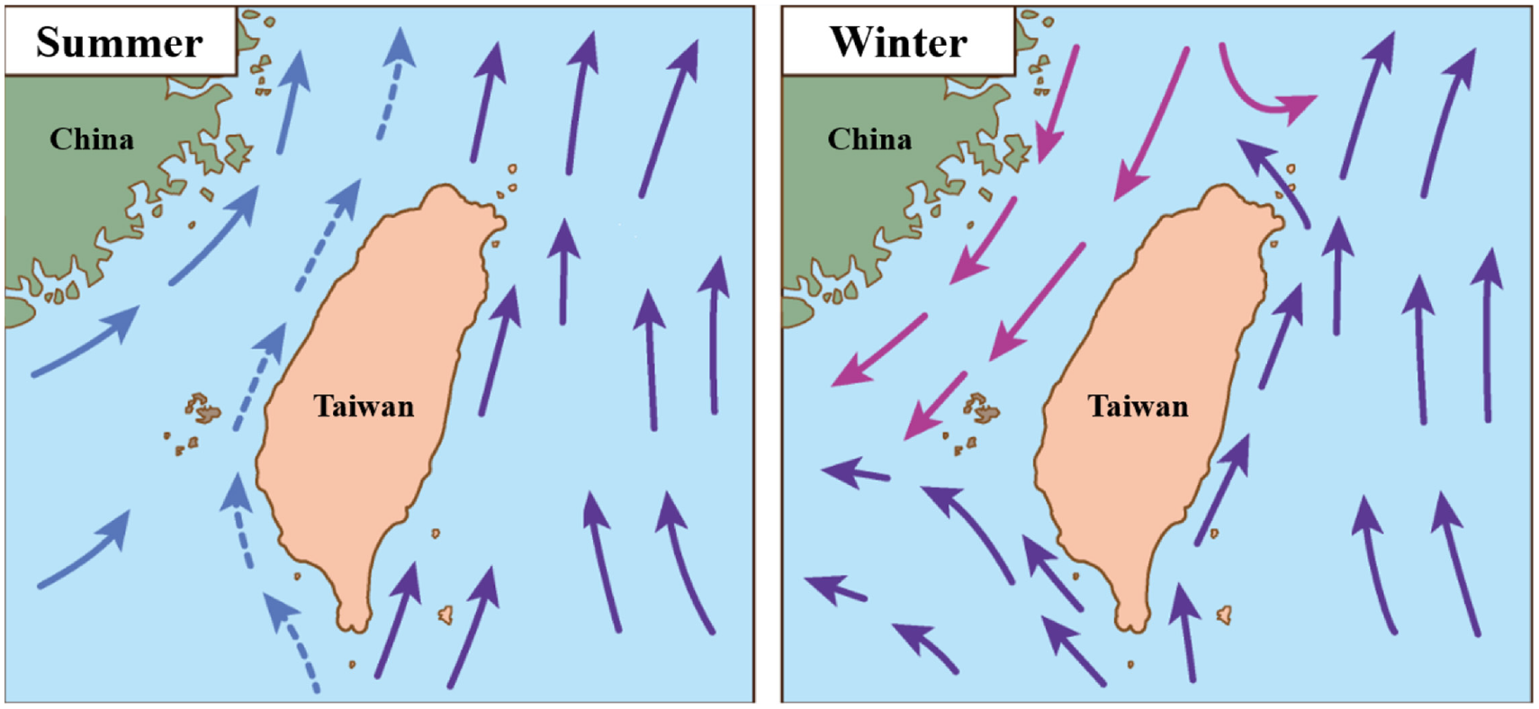
Seasonal wind flow pattern in Taiwan (Central Meteorological Bureau, 2020).
Wind forecasting research
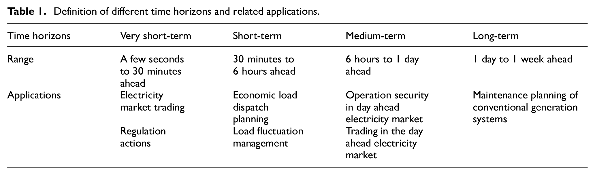
Wind forecasting can be divided into four general groups depending on the time horizon (Soman et al., 2010): (a) very-short term (a few seconds–30 minutes), (b) short-term (30 minutes to 6 hours), (c) medium-term (6 hours to 1 day), and (d) long-term (more than 1 day). The different applications for each time horizon are shown in Table 1.
Definition of different time horizons and related applications.
Researchers have used different methods to forecast wind speeds (Wu and Hong, 2007). These methods are classified into three general categories: (1) model-driven methods, (2) data-driven methods, and (3) ensemble methods.
The model-driven methods, such as the Numerical Weather Prediction (NWP), is based on meteorological physics and advanced mathematical models (Chen et al., 2014; Lange and Focken, 2006). This model requires the assimilation of large amounts of geometrical and meteorological data, including temperature, pressure, surface roughness, and characteristics of the region surrounding the wind farm. The NWP model usually provides high accuracy in terms of prediction, but requires a large amount of calculation time. Thus, these methods may not be practical for short-term forecasting.
Data-driven methods are based on historical data and finding the relationships between the input variables and a desired output. A data-driven method commonly consists of both statistical and artificial intelligence methods. Popular statistical approaches include the persistence model (Hu and Chen, 2018), the autoregressive moving average model (Erdem and Shi, 2011; Ezzat et al., 2018), and the autoregressive integrated moving average model (Ziel et al., 2016). On the other hand, the artificial intelligence method is based on several techniques used to deal with the non-linear problems. Typical artificial intelligence methods include the Artificial Neural Networks (ANN) (Liu et al., 2019), the Support Vector Machine (SVM) (Santamaría-Bonfil et al., 2016), the Extreme Learning Machine (ELM) (Luo et al., 2018; Zheng et al., 2017), and others (Abuella and Chowdhury, 2017; Lahouar and Ben Hadj Slama, 2017). In addition, deep learning models, such as the Long Short-Term Memory (LSTM) (Zheng et al., 2017), the Gated Recurrent Unit (GRU) (Syu et al., 2020), and the Deep Belief Network (DBN) (Wang et al., 2018), have been proposed as effective forecasting methods.
An ensemble method is a combination of either model-driven or data-driven methods with signal preprocessing techniques, machine learning techniques, or optimization algorithms (Li et al., 2019). Signal preprocessing techniques include the Wavelet Transform (WT), Empirical Mode Decomposition (EMD) (Zhang et al., 2016), and Kalman Filters (KF) (Chen and Yu, 2014). Machine learning techniques include K-mean Clustering, the Gaussian Process, and Stacked Autoencoders (SAE) (Tasnim et al., 2017). Optimization algorithms include genetic algorithms (GAs) (Lin et al., 2019), Grid Search (GS) (Zhang et al., 2014), and Particle Swarm Optimization (PSO) (Ren et al., 2014).
Research area and method
Observation site
The Taipower Meteorological Mast, which is operated by the Taiwan Power Company, is situated in the Chanbin area of Taiwan. It is located 6 km from the coastline of Fangyuan Township, Changhua county, as shown in Figure 2. In the geographic coordinate system, the mast is located at longitude 120°16′22″ E and latitude 24°0′23.4″ N.
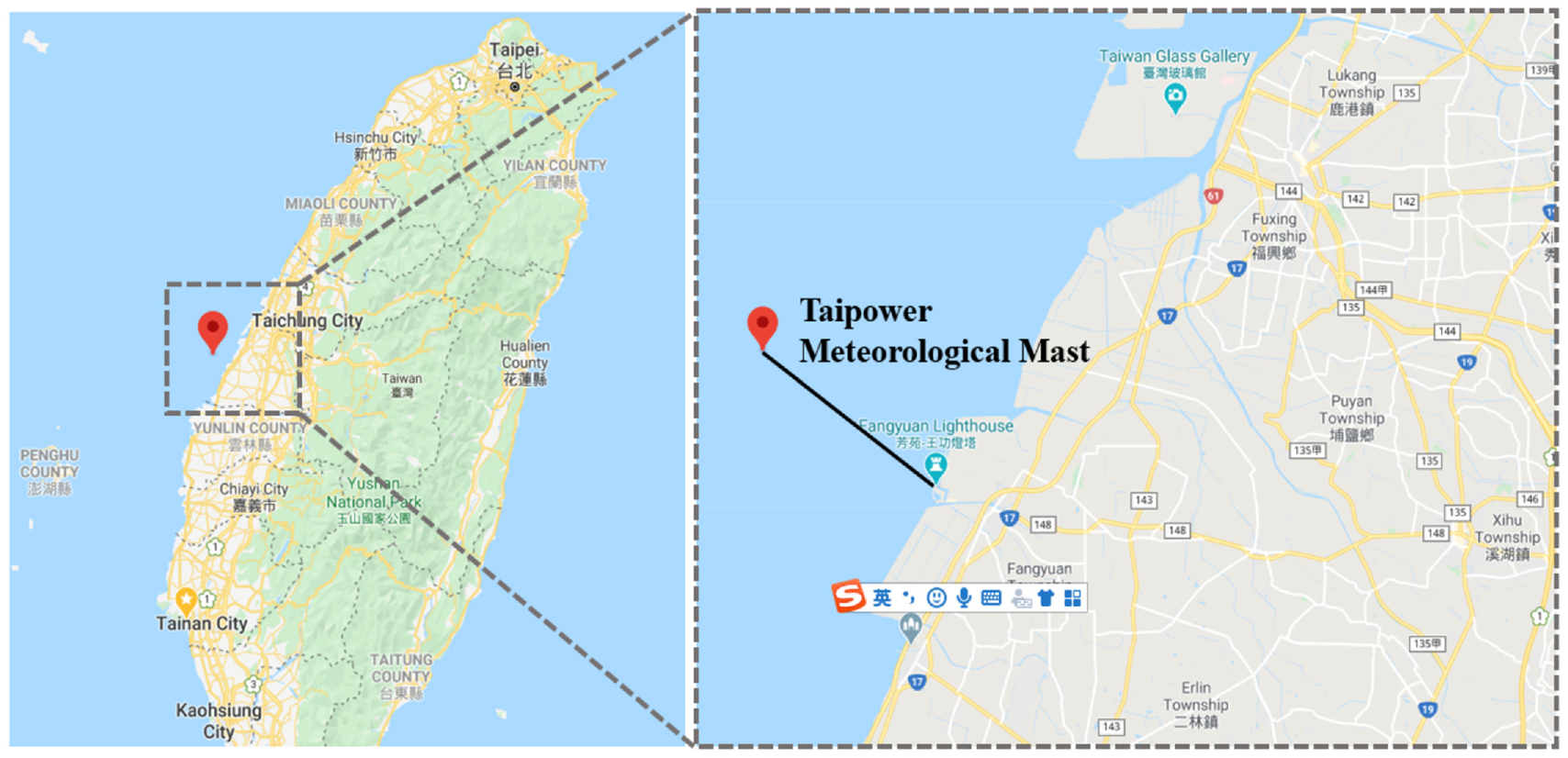
Location of the Taipower Meteorological Mast off the western coast of Taiwan.
The mast is 110 m in total height (95 m above sea level and 15 m below the surface of the water). Five cup anemometers and four wind vanes were installed at the following heights above sea level: 10, 30, 50, and 95 m. The position on the mast, where the measurements were taken, faced 150° to the southeast. The placement of the measurement equipment took into consideration the wind characteristics and the shading effects caused by the mast structure. If the installation of measurement devices were positioned in the northeast-southwest direction, the prevailing northeast wind in winter and the southwest wind in summer would produce a shading effect. In addition to the wind conditions, atmospheric and ocean surface properties including temperature, atmospheric pressure, precipitation, heat radiation, and wave conditions were recorded.
Proposed forecasting method
Artificial neural networks (ANN) have become the most popular technology used in solving forecasting and classification problems, and is inspired by biological neural networks. In simple terms, a neural-like network can be regarded as the ability to use algorithms to simulate the operations of biological nerves. This concept was first proposed by McCulloch and Pitts (1943), but was not widely applied until recently due to complex computations required. With improvements in the algorithms, hardware capabilities, and abilities to analyze big data, the multilayer neural network has become mainstream in artificial intelligence.
Based on the characteristics of wind speeds and directions of the study site, the Recurrent Neural Networks (RNN) was used. The purpose of RNN is to strengthen the training of the entire neural network model through time-series information. Simple RNN suffers from a vanishing and exploding gradients problem in the training process (Pascanu et al., 2013). In other words, RNN has poor performance in terms of long-term memory. The development of Long Short-Term Memory (LSTM), however, solves such problems by building deep, long-term memory cells in their structures (Chung et al., 2014).
The LSTM structure is shown in Figure 3 (Colah, 2015). The gates (input gate, forget gate, and output gate), which are composed of the sigmoid activation function (


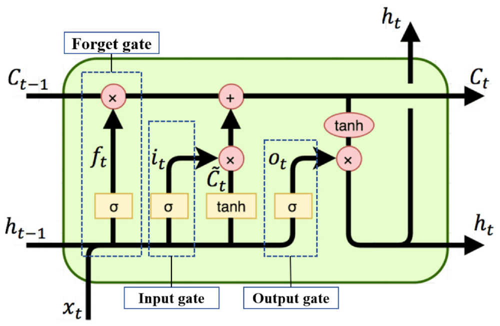
Structure of the LSTM cell, showing the location of the input, output, and forget gates.
where
Furthermore, to address model accuracy, three validation metrics were used in this study, including the Mean Absolute Error (MAE), Root Mean Squared Error (RMSE), and Normalized Mean Squared Error (NMSE). The MAE is the most commonly used evaluation index to measure the accuracy of a system. This metric can directly reflect the average error value for each prediction. The RMSE is aimed toward describing the model fit and is sensitive to outcome values. The NMSE shows the relative error among the prediction errors and variations in the data. It also equals to 1 −


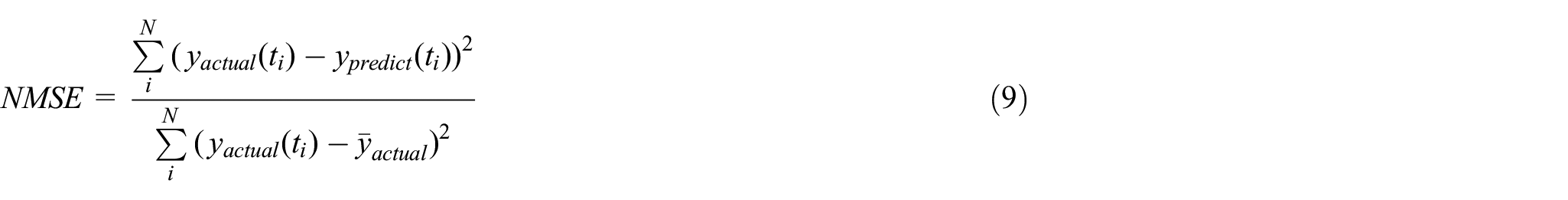
where
Results and discussion
The wind speed and wind direction data at the height of 95 m on the Taipower Meteorological Mast were used. This selection was based on the location of the sensors, which were nearest to the hub height of the currently planned offshore wind turbines and has high probability of being the standard for future offshore wind farms. The data in this research covered the period from January 2017 to December 2019, recorded at 1-second intervals and averaged into 1-minute intervals to reduce calculation times. The time series data foe wind speed and direction showed in Figure 4.
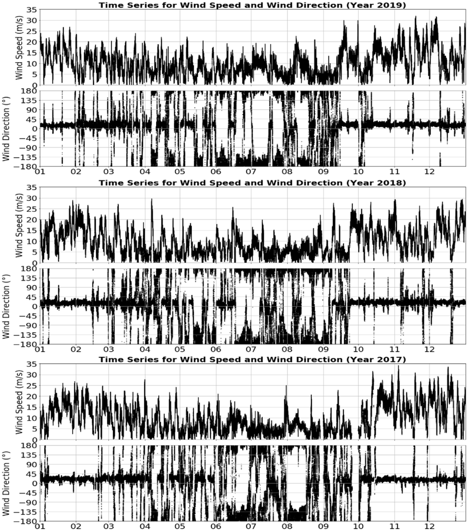
Time series for wind speed and direction (2017–2019).
Data statistics
The findings revealed that the 3 years studied were similar in terms of both wind speed and wind direction. An example is displayed in Figure 5, showing that the wind speeds were higher at the beginning and end of each year, especially in autumn and winter, with a monthly average wind speed of 12 m/s. The wind directions were consistent at the beginning and end of each year, and began to vary in the middle of February. Compared with the wind directions from October to February, the wind directions from March to September varied greatly. In addition, the mean wind direction was consistent at approximately 18° (N-N-E) in spring, autumn, and winter. In summer, the mean wind directions tended to be in a southwesterly direction (−160°), although the wind direction was not highly concentrated in a specific direction. This feature may indicate that the diurnal effect occurs in the southerly wind direction.
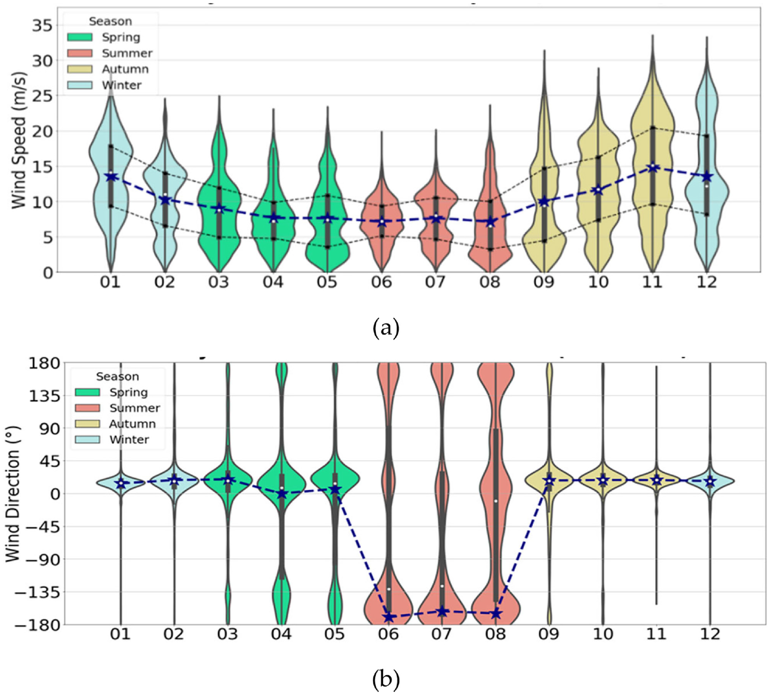
Violin plot of (a) wind speed and (b) direction in 2019.
Figure 6 shows that most of the high wind speed (>5 m/s) was northeasterly, from September to the following February. The Northeast monsoon ratio in Jan was 0.92 in April was 0.51, in July was 0.12, in Oct was 0.85. The wind speed distribution shifted into the low wind speed phase at the beginning of spring. The median value gradually decreased from approximately 13 m/s (winter season) to 7 m/s (spring season). At the same time, the wind direction distribution changed from the northeasterly wind and converged toward the southwesterly direction. The wind speed distribution was similar in spring and summer, but was different in terms of the direction. The results indicate that the overall wind speed intensity is highly related to the arrival of the northeast wind.
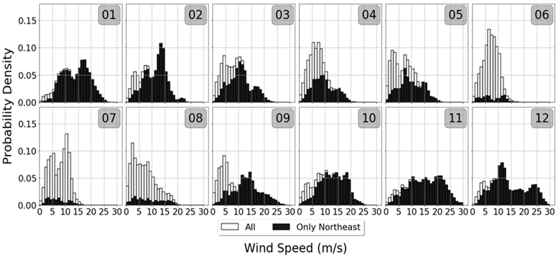
Histogram of wind speed in 2019 showing both all winds (white columns) and only winds from the northeast (black columns).
Forecasting results with the LSTM
The LSTM was chosen for this study because this model is currently the most widely used and most effective neural network model being utilized to analyze time series problems. During the machine learning phase, we split the 3-year data and used them as training, testing, and validating data, respectively. The training data was used for training the model and adjusting the parameters of the model. The testing data was used for evaluating the model parameters established during training, and the validating data was used to evaluate the model’s generalization.
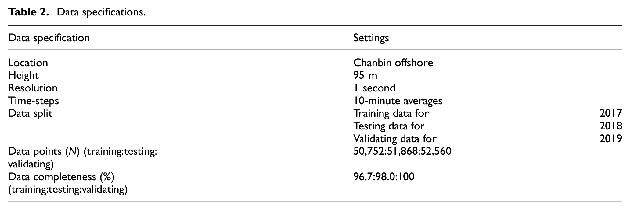
The data specifications for the training model are shown in Table 2. Because the prediction methods were based on a deep learning framework, and a large number of array calculations were necessary, we used Python, Tensorflow, and Keras as tools to carry out the algorithms and application of the model framework. Additionally, the CUDA and cuDNN frameworks were used. These frameworks helped to speed up the training progress by utilizing parallel GPU computations.
Data specifications.
The validation results can be divided into two parts, namely during the training process and after the training process. The validation of the training process results are shown in Figure 7, where the Mean Squared Error (MSE) epochs represents the number of iterations required for training. This situation indicated that the accuracy of the model had reached its limit. More epochs for training would only result in overfitting. Finally, we saved the model at epoch 143, which was the highest accuracy obtained in the testing dataset during the training process.
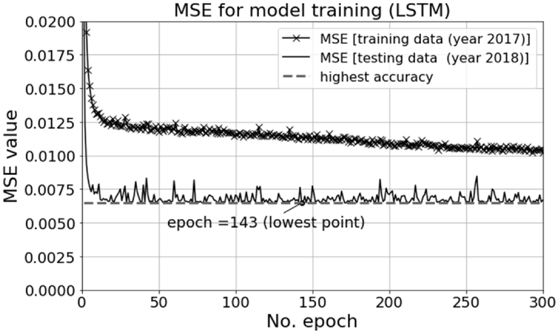
Results for the model training process.
N-step strategy (Ben Taieb et al., 2010; Wang et al., 2016) was introduced for forecasting. The recursive strategy uses the value forecasted in the current step as an input for the next step in the forecasting. The results of this strategy may suffer from poorer performance when the errors in each forecasting step accumulate (Ben Taieb et al., 2010). Time-steps of 10-minute averages were used in the forecasting model, and we found good performance of forecasting until third step prediction according to MAE and RMSE. Figure 8 shows the results for the data validation. First, further predictions resulted in larger errors in all situations. According to the MAE and RMSE results, the accuracy was lower in the summer and spring seasons. This situation may indicate that the prediction is more precise when there is a northeast wind, but less precise in the southeast wind period. This results could be compared with Figure 6. Apart from this, the NMSE results showed a greater difference in the accuracy in the spring and summer seasons. This result is not only due to lower accuracy but also because of greater variances in the validating results.
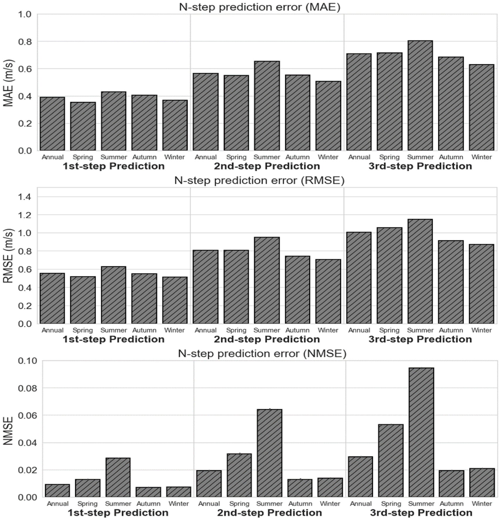
Validation results for MAE, RMSE, NMSE.
Figure 9 shows the results for the correlation plots comparing the predicted values with the actual values. The predicted values had a good fit with the actual values. The correlation values (
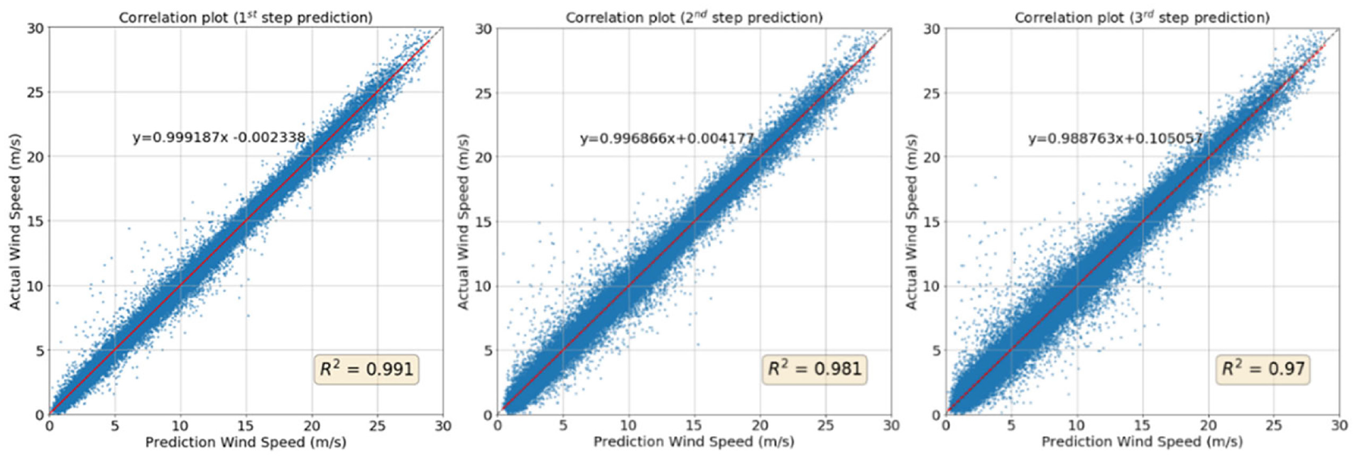
Correlation plot, first step prediction, second step prediction, and third step prediction.
Forecasting model test comparison
Three different models, namely the persistence model (PER), the Artificial Neural Network (ANN), and the Gated Recurrent Unit (GRU) were used to evaluate the performance of the LSTM model. Identical neurons, activation functions, and other hyperparameters were employed in this comparison.
Figure 10 shows the NMSE validation results. We found that the prediction errors of these four recurrent neural network models were not significantly different. Overall, the prediction errors were relatively higher in spring and summer. Due to a lack of variability in the outcomes, all four neural network models apparently had limited ability to handle large fluctuations. This suggests that highly variable wind conditions are difficult to train into these four relatively simple neural network models.
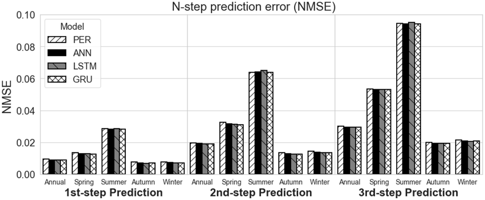
Model test validation (NMSE) prediction findings for the four forecasting models.
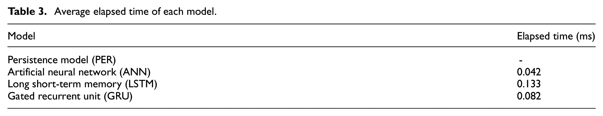
In addition, Table 3 shows the average elapsed time of each model. The overall prediction time averaged below 0.2 μs. This result indicates that the calculation time does not need to be considered due to the rapidity in predicting the next step value.
Average elapsed time of each model.
Time average test for LSTM
To observe differences in the LSTM model accuracy among different data intervals, we examined six time averages. For this evaluation, 2-, 5-, 10-, 15-, 30-, and 60-minute intervals were compared.
Figure 11 shows the performance for each time average, where overall a shorter time average was associated with higher accuracy. However, the accuracy was lower in the winter season, if the time average was shorter than 2 minutes. This is probably due to the turbulence effects experienced during this short-time interval especially in the high-speed wind regions. The turbulence effects affected the model in terms of precise forecasting. Thus, it is recommended that the selected time average should be longer than 2 minutes. Also, a longer time average resulted in larger errors overall. This is arguably due to discontinuity effects from the wind. When the time average is too long, therefore, prediction accuracy decreases.
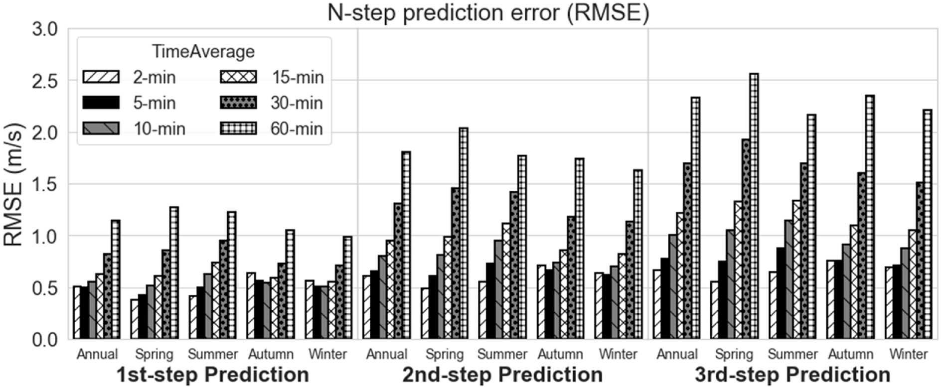
Time average validation results (RMSE) for the three-step prediction process.
Different time averages to forecast 30 minutes
Shorter time averages may increase the accuracy of the predictions, as discussed in the previous section. To predict a 10-minute time average, either a 1-step process involving 10-minute time averages can be used, or 2-step 5-minute time averages can be used. These two 5-minute time averages can then be averaged again into a 10-minute time average.
We chose a larger variation period in wind speed to observe these differences, with the time series prediction results displayed in Figure 12. We found that the prediction performance of the 2-step 5-minute time averages process was close to real data than 1-step 10-minute. This may be because the larger 10-minute time average will decrease the effects of short bursts of high-speed winds. Figure 13 shows the RMSE prediction errors of these 1- or 2-step forecasting procedures.
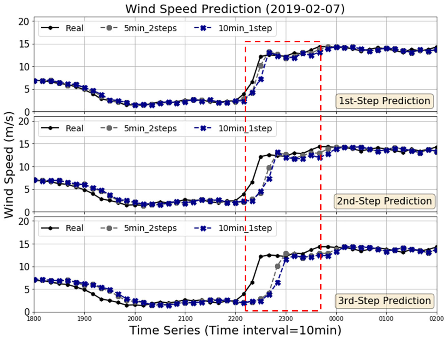
Three-step prediction in time series (time average comparison) for a total of 30 minutes.
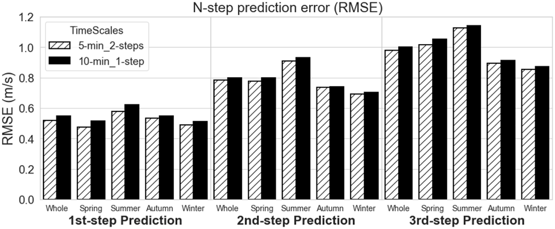
Ten-minute total averages in different time scale validations for a total of 30 minutes.
Conclusions
In this research, offshore wind data for the Taiwan Strait over a 3-year period (2017, 2018, and 2019) was used to develop an LSTM neural network forecasting model.
The statistical results identified seasonal characteristics. During the 3 years under observation, the trends in wind speeds were similar, but the arrival time of the northeast monsoon winds differed. The wind speeds were high in autumn and winter. Spring and summer were similar in terms of wind speeds, but there were differences in the wind directions. The wind direction also had larger variances in summer and spring than autumn and winter. In summary, the northeast monsoon winds in autumn and winter were steadier in terms of both speed and direction than the winds in spring and summer. Thus, offshore wind power generation will be more efficient in autumn and winter with the northeast monsoon winds.
The LSTM wind speed forecasting model was tested to examine the resulting errors. The errors mostly occurred during periods of discontinuity in both wind speed and wind direction. Furthermore, the accuracy was relatively low during the high-speed wind periods and the southwest wind periods. The annual correlation values for the three steps used in this prediction were 0.991, 0.981, and 0.970, respectively. This prediction accuracy was quite high, although sudden short bursts of high speed winds adversely affected these predictions. However, the accuracy of forecasting model could be significantly improved by shortening the data time average period (above 2-minute time average) or by dividing the prediction time into more steps.
Footnotes
Declaration of conflicting interests
The author(s) declared no potential conflicts of interest with respect to the research, authorship and/or publication of this article.
Funding
The author(s) disclosed receipt of the following financial support for the research, authorship and/or publication of this article: This work were supported by the Ministry of Science and Technology, Taiwan(MOST97-2221-E-168-043) and Taipower company.