Parameters estimation of a steady-state wind farm wake model implemented in OpenFAST

Abstract

Wake models play a fundamental role in predicting loads and power generated by wind farms. Using them, it is possible to assess how wakes develop and interact with each other and what are the effects generated in the context of a real operating farm. In this paper, a Gaussian Wake Model implemented in OpenFAST is validated against experimental data gathered in wind tunnel GVPM @ Politecnico di Milano in the context of the European CL-Windcon project. The software used to reproduce the mechanical dynamics of the G1 wind turbines is OpenFAST. It is coupled with FLORIS, a NREL’s software based on the Gaussian Wake Model, that allows to simulate the wake and partial wake conditions. The rotor aerodynamics is calculated using the BEMT on the actual rotor flow field. However, to properly use OpenFAST and the coupled GWM, eight parameters have to be estimated. Thus, a Least Squares Minimization procedure is performed using the available experimental data.

Keywords

Wind farm wake model wind farm control wake model validation Gaussian wake model

Introduction

The clustering of wind turbines is an advantageous practice from an economic point of view. However, the interaction between the turbine blades and the wind produces a wake that negatively affects the electrical power produced in the entire wind farm.

The wakes are characterized by a strong deficit in the wind speed acting on downstream turbines and an increased turbulence intensity with respect to the undisturbed flow. The velocity deficit usually limits the power production of the wind turbines placed downwind as showed in Barthelmie et al. (2009), Vermeer et al. (2003), and Porté-Agel et al. (2013) The increase in turbulence instead enhances the fatigue loads on structural components leading to a reduced operational life of the machine. For these reasons, adequate control techniques that take into account the wind farm operating conditions as a whole system are needed in contrast to approaches that only consider the single turbine. These control methods, in order to be efficient, need an accurate prediction of the wakes developed within the farm. Several wake prediction methods have been proposed in the last few years. They can be grouped based on their level of complexity and fidelity. The main distinction is between high-fidelity and low-fidelity models.

High-fidelity wake models are usually based on the Computation Fluid Dynamics (CFD) approach. They can describe accurately the phenomenon investigated since they are based on the law of physics (conservation of energy, momentum, etc…). The state of the art of such methods, as of today, is represented by the coupling between OpenFAST (NREL), a NREL’s mechanical dynamics simulator for wind turbines, and OpenFOAM (2020)/SOWFA (NREL). OpenFOAM (2020) is a well-known open-source CFD solver, while SOWFA (NREL) (2020) is a NREL’s library developed ad-hoc for OpenFOAM (2020) that allows for the simulation of the Atmospheric Boundary Layer (ABL) and the wakes generated inside a 3D domain where the wind farm is simulated. Currently, the fluid-blade interaction is evaluated by means of an Actuator Line Model (ALM) that is used to model the forces exchanged between them by means of point forces smeared in the domain through a kernel function (usually it has an exponential shape). In this way, discontinuities that could undermine the correct behavior of the numerical method are avoided. A detailed description of the ALM theory can be found in Schito and Zasso (2014). Other high fidelity models available for simulating wind turbines with the aid of CFD are the Actuator Disk Model (ADM) and the Vortex Wake method. In the ADM the rotor is modeled as a permeable disk, while in the Vortex wake method the rotor blades and the trailing and shed vortices (in the wake) are represented by lifting lines or surfaces as explained by Srensen (2012). Such methods are essential when studying the wake interaction and development phenomenon that takes place in large wind farms.

However, they cannot be used for controlling in real time the wind farm (or even a single turbine). In this case, the only available option is to renounce some of the model complexity to obtain the information we need in an useful time frame. The models that accomplish this goal are usually termed as low-fidelity.

Such models are typically analytical or experimental. They give a rough, but rapid estimation of the flow field acting in a given wind farm configuration. As already said, they are of fundamental importance in the industrial practice for the evaluation and estimation of turbine performances. The state of the art for these kind of models is given by the open-source control-oriented software FLORIS (NREL), developed by NREL. It is based on the Bastankhah and Porté-Agel (2014, 2016) GWM and is able to output the full flow field developed in a wind farm whose specifics are specified by the user. A $C_{T} - TSR$ table of the turbines composing the wind farm is needed too. The natural extension of FLORIS (NREL) to a dynamic model is given by FloriDyn (Becker) (2020), Gebraad and van Wingerden (2014), and Farrell et al. (2021). It shares the same GWM model for the evaluation of the wake deficit and deflection, but uses the newly introduced concept of Observation Points (OP) to evaluate the transport dynamics of the wake. More details can be found in Gebraad and van Wingerden (2014). Obviously this model is more computationally demanding than the standard FLORIS (NREL) (2020), but it is, as of now, one of the very few dynamic control-oriented models. It can be used to test new promising dynamic control strategies that are emerging nowadays in the context of wind farm control.

Aside from these two (that represent the best for low-fidelity models), the literature is full of well-known models. For example there is the Jensen (1983) 1-D model that assumes a top-hat shape for the wake speed deficit and a linear spread of the wake. It is based on the linear momentum conservation like the Frandsen et al. (2006) model. A more refined wake model based on Jensen (1983) is the Zone model developed by Gebraad et al. (2014, 2016). It divides the wake in three sections (or zones). They are the near wake, far wake and mixing zone. Each of them has a characteristic expansion factor of the wake diameter. The Zone model (Gebraad et al., 2014, 2016) lays the foundation for the Bastankhah and Porté-Agel (2014, 2016) GWM model.

Of course, the distinction between high and low fidelity is only qualitative. In the middle, different models that are a compromise between these two worlds exist. The wake model validated in this work, although based on the GWM model, is more advanced thanks to its direct coupling to the OpenFAST (NREL) (2020) aero-elastic code. More details about it can be found in Cioffi et al. (2020).

Aside from the model (explained in detail in section Reviewing the GWM for OpenFAST) that will be validated in this paper, in the mid-fidelity area we can already find the Dynamic Wake Meandering (DWM) model developed at DTU by Larsen et al. (2007) and the WindFarmSimulator (WFSim) developed at TU Delft. A simplified version of the Navier-Stokes equations are used in the DWM. The model, as can be easily inferred from the name, is able to reproduce the wake meandering phenomenon. WFSim is based on the Navier-Stokes equations, too. However, the 2-D version of the equations were used. As of today, FLORIS (NREL) and WFSim are the most employed tools to develop new control algorithms. van Dijk et al. (2017) and Bay et al. (2019), thanks to these softwares, supported the concept of secondary steering and showed how through wake steering it is possible to perform multi-objective optimization for wind farm control.

In this paper a wake model proposed by Cioffi et al. (2020) based on the coupling of OpenFAST (NREL) and the GWM will be briefly reviewed. The results obtained will be compared and validated against the experimental data gathered using the G1 turbine in the GVPM Wind Tunnel of Politecnico di Milano within the European CL-Windcon (2020) project. The article is organized in the following way. First, a brief review of the GWM model will be presented. Then the Wind Tunnel Setup and the Numerical Model Setup will be discussed. Finally, the parameters estimation and model validation will be described in detail together with the major conclusions drawn and the future work that could be performed.

Theory

In this section the theory of the Bastankhah and Porté-Agel (2014, 2016) GWM model will be briefly presented, together with the changes that have been made to it. For a complete analytical description of the model, please refer to Bastankhah and Porté-Agel (2014, 2016) and Cioffi et al. (2020).

Gaussian wake model

Bastankhah and Porté-Agel (2014, 2016), after performing a budgeting study of the Reynolds Averaged Navier-Stokes Equations (RANS), proposed the hypothesis that is at the basis of the GWM theory. The hypothesis is that the wake generated by a wind turbine in the far field shows a self-similarity characteristic. This means that, by normalizing the wake velocity deficit measured at a far distance from the wind turbine rotor, the same characteristic curve is always obtained. The authors proposed a gaussian shape to fit the characteristic curve. This choice was motivated by the fact that the gaussian is able to copy in an accurate manner the self-similar curve up to a relative yaw angle (with respect to the wind) of the turbine rotor of 30°. Together with the wake deficit profile, the authors developed a formulation for the wake deflection too.

Equations (1) and (2) show the formulas to evaluate the wake velocity deficit and deflection at a certain point (x,y,z) behind the rotor.

\frac{\bar{u} (x, y, z)}{u_{\infty}} = 1 - C (x) e^{\frac{- {(y - δ)}^{2}}{2 σ_{y}^{2}}} e^{\frac{- {(z - z_{h})}^{2}}{2 σ_{z}^{2}}}

(1)

\frac{θ (x, y, z)}{θ_{m}} = e^{\frac{- {(y - δ + σ_{y})}^{2}}{2 σ_{y}^{2}}} e^{\frac{- {(z - z_{h})}^{2}}{2 σ_{z}^{2}}} and θ_{m} = \frac{θ_{c}}{e^{- 0.5}}

(2)

In equation (1), $\bar{u}$ represents the velocity in a (x,y,z) point behind the turbine’s rotor, $C (x)$ is the normalized velocity deficit at the wake center as function of the x coordinate (downstream distance from rotor), $σ_{y}$ and $σ_{z}$ are the wake widths in $y$ and $z$ direction, $z_{h}$ is the hub height of the turbine and $u_{\infty}$ is the undisturbed flow velocity. In equation (2), $δ$ stands for the wake center deflection while $θ_{c}$ is wake skew angle of the wake center. $σ_{y}$ and $σ_{z}$ have been modeled by the authors using a linear formulation (validated by wind tunnel tests as discussed in Bastankhah and Porté-Agel (2014, 2016) that is function of the downstream distance from the turbine’s rotor and of the turbine yaw angle:

\frac{σ_{z}}{d} = k_{z} \frac{x - x_{0}}{d} + \frac{σ_{z 0}}{d}

(3)

\frac{σ_{y}}{d} = k_{y} \frac{x - x_{0}}{d} + \frac{σ_{y 0}}{d} and \frac{σ_{y 0}}{d} = \frac{σ_{z 0}}{d} \cos γ

(4)

k_{y} = k_{z} = k_{a} I + k_{b} and k_{a} = 0.38371, k_{b} = 0.003678

(5)

In equations (3)–(5), $d$ is the turbine’s diameter, $x_{0}$ is the downstream distance where the far wake zone ideally begins, $σ_{y 0}$ and $σ_{z 0}$ are the wake widths at the far wake zone beginning, $k_{z}$ and $k_{y}$ are two constants function of the wind turbulence intensity $I$ , $k_{a}$ , and $k_{b}$ are two pure constants and $γ$ is the relative yaw angle of the turbine with respect to the incoming flow.

Equations (6) and (7) report the normalized velocity deficit $C (x)$ at the wake center together with the wake deflection $δ_{0}$ relative to the rotor axis at the beginning of the far wake zone. The complete derivation of these expression is not showed here for the sake of brevity, but it is available in Bastankhah and Porté-Agel (2014, 2016).

C (x) = 1 - \sqrt{1 - \frac{σ_{y 0} σ_{z 0} M_{0}}{σ_{y} σ_{z}}}

(6)

\begin{array}{l} δ = δ_{0} + \frac{θ_{c 0} E_{0}}{5.2} \sqrt{\frac{σ_{y 0} σ_{z 0}}{k_{y} k_{z}} M_{0}} \\ \times \ln \frac{(1.6 + \sqrt{M_{0}}) (1.6 \sqrt{\frac{σ_{y} σ_{z}}{σ_{y 0} σ_{z 0}}} - \sqrt{M_{0}})}{(1.6 - \sqrt{M_{0}}) (1.6 \sqrt{\frac{σ_{y} σ_{z}}{σ_{y 0} σ_{z 0}}} + \sqrt{M_{0}})} \end{array}

(7)

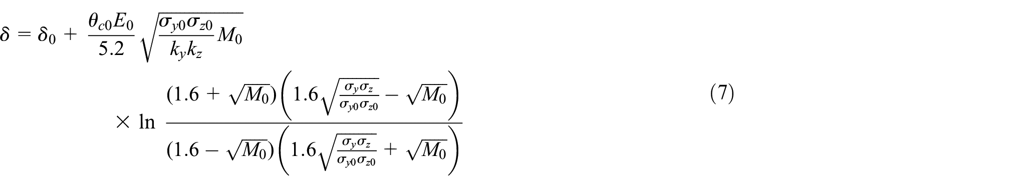
In equations (6) and (7), $M_{0}$ and $θ_{c 0}$ are respectively the wake deficit speed and skew angle of the wake center at the beginning of the far wake region. A complete explanation of how the parameters referring to the beginning of the far wake region (the ones with the 0 subscript) are obtained we refer once again the readers to Bastankhah and Porté-Agel (2014, 2016).

Up to now, the GWM equations presented are referred to the wake generated by a single turbine. Of course, they can be used also for the case of a wind farm. However, some additional considerations have to be done when using the GWM for this purpose. Typical problems to be addressed in this case are the interaction between wakes that could happen due to the geometry of the farm and the added turbulence intensity generated by wake mixing.

In FLORIS (NREL), the wake interaction problem was solved adopting a correction developed by Katic et al. (1987). The author proposed that the square of the wake deficit at a certain downstream position is equal to the squared sum of the wake deficit generated by the single turbines upwind. For what regards the added turbulence intensity, the method proposed by Crespo and Hernandez (1996) was implemented. The authors propose an empirical formulation of the added turbulence due to the wake generation and mixing in the free-stream velocity. Its formulation is reported in equation (8), where $I_{0}$ is the ambient turbulence intensity referred to the free stream condition and $C_{I}$ , $e_{1}$ , $e_{2}$ , and $e_{3}$ are parameters to be determined experimentally.

I_{+} = C_{I} A_{ol, %} a_{i}^{e_{1}} I_{0}^{e_{2}} {(\frac{x}{D_{i}})}^{e_{3}}

(8)

The added turbulence is deemed proportional to the product of the free-stream turbulence, the normalized downstream distance considered, the Axial Induction Factor (AIF) of the turbine considered and the ratio of overlapping area between the rotor of a turbine and the wake area generated by upstream turbines. Each of this terms has been raised to a power whose exponent was determined experimentally. For the turbulence intensity $I$ , due to the wake’s superposition, a correction by Niayifar and Porté-Agel (2015) was implemented. The method is analogous to the one proposed by Katic et al. (1987) for evaluating the wake deficit at a given downstream distance.

In FLORIS (NREL), an additional empirical correction on the $C_{P}$ and $C_{T}$ is used to evaluate the power extracted from a yawed turbine. This correction won’t be needed anymore with the GWM implemented in OpenFAST (NREL) since the aero-elastic code is capable of directly evaluate the $C_{P, yaw}$ and $C_{T, yaw}$ .

Reviewing the GWM for OpenFAST

Since OpenFAST (NREL) is able to directly output the $C_{T}$ and AIF on the whole rotor plane (unlike FLORIS (NREL) that uses a $C_{T} - TSR$ table) at each time step of simulation, it is now possible to review the GWM to implement it in the aero-elastic code.

The major difference with the model proposed in Bastankhah and Porté-Agel (2014, 2016) is that now the AIF and $C_{T}$ are two separate entities that don’t rely on the simplified relationship reported in equation (9).

C_{T} \approx 4 a (1 - a \cos γ) and a \approx \frac{1}{2 \cos γ} (1 - \sqrt{1 - C_{T} \cos γ})

(9)

For a more detailed description of the GWM changes, please refer to Cioffi et al. (2020). The corrected GWM model can now be implemented in the InflowWind module of OpenFAST (NREL).

The wind calculation routine at a generic time step works as follows. After identifying the most upstream turbine, the model evaluates the free-stream wind speed on the turbine’s rotor. In this way, the aerodynamics of the machine can be solved using the BEMT. Then the $C_{T, i}$ of the current turbine (that is the most upstream turbine denoted by subscript $i$ ) and the AIF on the whole rotor plane is obtained. Now we can pass to the first downstream turbine (that from now on will be denoted by subscript $i$ , while the turbine formerly analyzed will now be denoted by subscript $i - 1$ ). Again, the GWM supplies the wind speed on the whole rotor plane of the machine. To do so, the $C_{T, i - 1}$ and the rotor-plane averaged AIF $a_{i - 1}$ of the first turbine are needed. The $C_{T, i}$ and $a_{local, i} (r)$ can now be evaluated. The same steps are performed for all the machines composing the wind farm throughout the entire simulation.

Wind tunnel setup

The cases analyzed in the experimental setup (and that will be reproduced in the numerical simulations) are part of an experimental campaign performed in the Galleria del Vento Politecnico di Milano (GVPM) in the context of the European CL-Windcon (2020) project, whose main objective is the development of new, advanced control logics able to optimize power extraction and load mitigation in both onshore and offshore wind farm contexts. The wind tunnel tests have been performed at the well known Galleria del Vento Politecnico Milano (GVPM). It is a closed-circuit wind tunnel arranged in a vertical layout with two test rooms located on the opposite sides of the loop. The first one is located in the lower part of the loop, suitable for Low Turbulence tests, while the second one, bigger, is located in the upper part of the loop, suitable for Boundary Layer tests. The facility is powered by 14 1.8m fans with a power of 100 kW each and a total power of 1.4 MW. The CL-Windcon (2020) tests are performed in the Boundary Layer Test section which is 13.84 m wide and 3.84 m high and is specifically designed for wind engineering test structures subject to atmospheric flow conditions.

Wind farm layout

The machine used to perform the test is the Generic 1.1 m diameter rotor $(D = 1.1 m)$ , also called G1 (for a detailed description of the turbine characteristics, please refer to CL-Windcon (2020)). It is a scaled turbine realized in collaboration with TU-Munich. The model was conceived with the following characteristics:

a realistic energy conversion process enabled by good aerodynamic performances;

active pitch, yaw and torque control to allow control strategies testing;

a comprehensive on-board instrumentation;

dimensions allowing a good compromise between the need for miniaturization, wind tunnel blockage, Reynolds number effects and the need to realize one-to-one or multiple wind turbine interference conditions typical of wind farm operations.

The G1 turbine has a hub height of $z_{hub} = 0.825 m$ , a rated rotor speed of $Ω_{rated} = 850 rpm$ , three blades composed by layers of unidirectional carbon fiber covering a machined Rohacell core. The turbine is very small, so that the rotor airfoils can operate in a low Re regime. Because of its small size, the turbine can be considered to be a rigid body, especially during steady-state simulations as those presented in this paper. Various tests have been performed during this experimental campaign, but the most relevant for the present work are two:

the tests performed using a single G1 turbine;

the tests performed using a series of 2 G1 turbines aligned in the flow direction with a relative distance of 5.5 m (5 G1 rotor diameters) and with the first upwind G1 turbine presenting various yaw angles different from 0° (various yaw misalignment angles with the incoming flow).

The coordinates of the hub center point of the turbines arranged in a 2 × 1 wind farm configuration can be found in Table 1 together with a graphic representation reported in Figure 1.

Table 1.

The 2 × 1 wind farm configuration in absolute and dimensionless values.

Wind farm layout
-	x [m]	y [m]	z [m]	x/ $D$	y/ $D$	z/ $D$
T1	0	0	0.825	0	0	0.75
T2	5.5	0	0.825	5	0	0.75

Figure 1.

2 × 1 G1 wind farm layout (obtained with FLORIS (NREL)).

Wind tunnel flow characteristics

As stated in the previous subsection, two sets of wake measurements have been selected from the CL-Windcon (2020) campaign to perform the parameters estimation of the OpenFAST (NREL)/GWM coupled model.

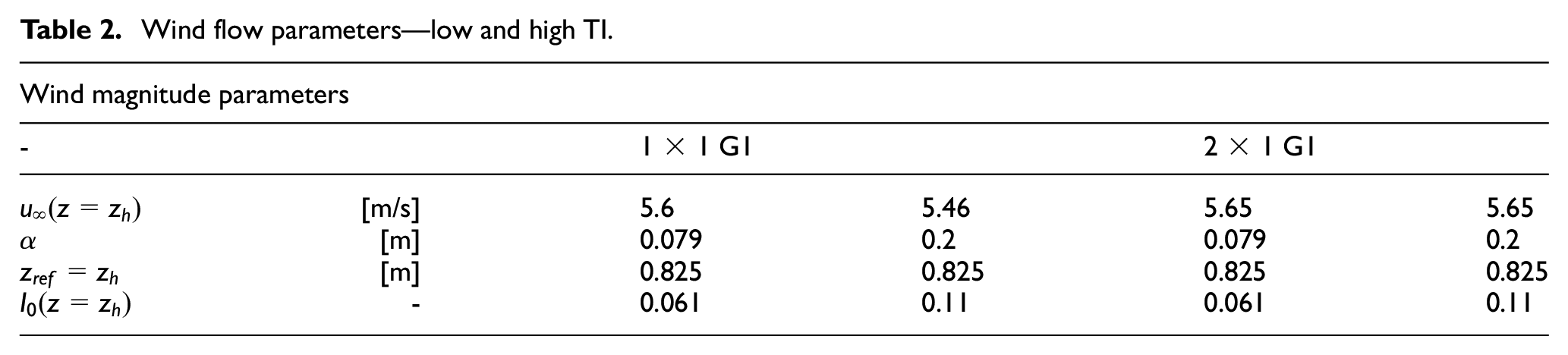
The first set is the one related to the single G1 turbine (1 × 1 G1). In this case, the GVPM has been operated in order to obtain two different subsets of measurements. The first subset has an incoming power law wind profile having a wind speed of 5.6 m/s at the hub of the G1 turbine, a wind shear exponent of 0.079 and a Turbulence Intensity (TI) of 6.1%. The second subset has an incoming power law wind profile having a wind speed of 5.46 m/s at the hub of the turbine, a wind shear exponent of 0.2 and a Turbulence Intensity (TI) of 11%. The various measurements have been performed by yawing the G1 turbine at various angles with respect to the incoming undisturbed wind flow (the yaw angle interval goes from [−30,30]° with a regular span of 10°).

The second set (wind farm configuration) has two G1 turbines aligned in the flow direction and distant 5 G1 diameters one from the other (2 × 1 G1). In this case, the GVPM has been operated in order to obtain two different subsets of measurements. The first subset has an incoming power law wind profile having a wind speed of 5.65 m/s at the hub of the turbine, a wind shear exponent of 0.079 and a Turbulence Intensity (TI) of 6.1%. The second subset has an incoming power law wind profile having a wind speed of 5.65 m/s at the hub of the turbine, a wind shear exponent of 0.2 and a Turbulence Intensity (TI) of 11%. The various measurements have been performed by yawing the two G1 turbines at various angles with respect to the incoming undisturbed wind flow (the considered yaw cases only include 0° and 30° values to limit the number of wind tunnel tests to be performed).

The inflow characteristics for the set of tests are reported in Table 2

Table 2.

Wind flow parameters—low and high TI.

Wind magnitude parameters
-		1 × 1 G1		2 × 1 G1
$u_{\infty} (z = z_{h})$	[m/s]	5.6	5.46	5.65	5.65
$α$	[m]	0.079	0.2	0.079	0.2
$z_{ref} = z_{h}$	[m]	0.825	0.825	0.825	0.825
$I_{0} (z = z_{h})$	-	0.061	0.11	0.061	0.11

Wind tunnel measurements and results

In Figure 2 is reported a schematic view of the downstream wake points that have been measured in the context of the experimental campaign. From a quantitative standpoint, data was gathered at 5D, 7.5D, and 10D downstream the single G1 turbine. The recorded data comprehends wake velocity in x-y-z directions, structural and aerodynamics loads that were acting on the blades of the turbines (these data could come in very useful when validating the wake model in terms of loads acting on the blades), control variables (like pitch angle of the blades, rotating speed of the rotor and its torque) and several others that are contained in databases. These databases are the final output of the experimental campaign, together with some deliverables that explain in detail the experiments and tests performed. The measurements where obtained by means of hot wire anemometers MODEL: 90C10 CTA working at a frequency of 1000 Hz (or Cobra probes made by TFI instruments) covering points located at the cited downstream locations and at specified locations in these planes.

Figure 2.

Points where flow velocity has been measured in the experimental campaign.

The same setup was adopted for the case of the wind farm configuration, but of course this time the planes on which data was recorded are different. Data was gathered at 7.5D and 10D from the first G1 turbine. A useful remark to be kept in mind is that usually, at a distance of 5D the wake of the upwind turbine is considered to be in the far-wake zone. In such zone, the wake develops fully into a self-similar Gaussian profile (this is from where GWM model takes its name). The G1 turbines are operated in all the tests at the limit of the region II of the generator control, so that no pitch control is needed to let them work correctly. Where pitch variations had been observed (due to the turbulent nature of the flow which makes the turbine work in region III) the mean value of the angle (and other needed varying quantities) has been taken.

Numerical setup

In this section, the numerical setup of the OpenFAST (NREL) simulations, using the implemented GWM model, is proposed. The G1 model for the OpenFAST (NREL) software was obtained thanks to TU Munich prof. Campagnolo, that had already validated such a model against wind tunnel tests executed at GVPM. The hardest modeling issue was finding the aerodynamic coefficients of the G1 blade’s sections at various Reynolds numbers in order to have a reliable model in all conditions. To be able to use such lookup tables, a change in the OpenFAST (NREL) software was necessary. This allowed OpenFAST (NREL) to correctly read such tables, interpolate them and use the values to evaluate the BEMT on each airfoil section. The control logic of the generator used in the wind tunnel test was missing. It has been replaced by a simple Rotor Power—Rotor Torque quadratic curve (set-points reproducing the real working of the machine). For some tests this curve was not used and the rotor speed was simply kept as constant (the rotor speed was no more a degree of freedom of the multibody model, but a simple kinematic constraint). The wind farm configuration and the wind input characteristics employed in the numerical simulations are the same mentioned in SubSect. Wind Farm Layout and SubSect. Wind Tunnel Flow Characteristics. For what regards the free-stream inflow, a power law profile was used (more details about it can be found in the EUROCODE EN 1991-1-4:2005(E) (2005)).

Multibody simulation settings

For the purposes of the current simulation, a multibody wind turbine model has been used. The software that implements it is OpenFAST (NREL). It is composed of various modules that simulate different physical phenomena. The modules used in this work are:

ElastoDyn (responsible for the structural behavior of the machine)

InflowWind (responsible for generating the flow field surrounding the machine)

AeroDyn v15 (responsible for the aerodynamics of the machine)

ServoDyn (responsible for the control part of the machine)

In the ElastoDyn input file, various changes were made based on the experimental tests that had to be reproduced. In this file it is possible to specify what are the Degrees of Freedom (DOFs) activated in the simulation. As already said in section Numerical Setup, the rotor speed was kept fixed in all the simulations. However, to test the correct working of the Rotor Torque—Rotor Speed table, a simulation was performed with the Generator DOF activated so as to control the low speed rotor angular velocity. In this case the machine behaved as prescribed by the table and a transient period was observed before the rotor reached the correct rotational velocity (wrong initial condition was imposed). The low speed rotor angular velocity set point is mainly a function of the incoming wind speed and of the yaw angle of the machine. Another DOF that was active during the simulations was the Yaw DOF.

In the InflowWind Module, the wind model employed is the GWM described in section Reviewing the GWM for OpenFAST. This model was used for both the single G1 (1 × 1 G1) turbine and the 2 × 1 wind farm configuration cases (2 × 1 G1). To run it, it is necessary to specify some input parameters like the undisturbed wind speed and shear, the wind direction, the layout of the wind farm and the GWM model parameters for a correct evaluation of the wake.

In the AeroDyn v15 input file the necessary parameters for the aerodynamic simulation (BEMT model) were set. Since the GWM is a stationary model, a classic BEMT was adopted. The maximum number of iterations allowed for convergence of the AIF and TIF (activated in the simulation) was set to $n_{it} = 10000$ . Glauert’s Tip Loss and Hub Loss corrections were activated in the simulation. For the blade’s airfoil aerodynamics, the steady option was used (no unsteady aerodynamics). Finally, to keep into account for the effect that the skewed wake has on the yawed turbine, the Pitt and Peters (1981) BEMT correction is activated. As specified in section Numerical Setup, the most important modeling part for the G1 turbine on OpenFAST (NREL) regarded the airfoil polars. More details about this can be found in Campagnolo et al. (2019). These tables divide the blade in 40 different sections. For each of them, a 2D polar, function of both the Angle of Attack and the Reynolds number of the incoming flow acting on the section, is specified. In order to be able to use properly these tables a change was made to OpenFAST (NREL) source code. In this way, at each time step, the software is able to perform the evaluation of such coefficients and use them to evaluate the BEMT.

Parameters estimation and model validation

The main objective of the work is the validation of the GWM model coupled to OpenFAST (NREL) by means of comparison of the predicted analytical wake with the ones measured experimentally during the CL-Windcon (2020) campaign. As of now, the GWM model was run using some basic parameters found in literature and proposed by Bastankhah and Porté-Agel (2014, 2016) and Campagnolo et al. (2019). From the work of Campagnolo et al. (2019), it is possible to see that, by carrying out a Least Square Minimization (LSQ) procedure on the GWM model, using the gathered data it is possible to find out the optimal parameters that reduce the model error with respect to the gathered data. However, Campagnolo et al. (2019) and Bastankhah and Porté-Agel (2014, 2016) results were obtained for a single turbine. In the present work, the parameters estimation will be presented for both a single G1 turbine and for the 2 × 1 G1 wind farm configuration. The latter case is of fundamental importance because allows for a more realistic validation of the model. The single turbine case is quite limiting and does not keep into account for a variety of phenomena that happen when considering a real wind farm, like the wake superposition or the partial wake covering of a downstream rotor. This is why the parameters obtained in this study should be more representative of a real operating wind farm. However, as already said, the parameters will be at first optimized using the single turbine case so as to verify that the results obtained from Matlab’s minimization procedure are consistent with the ones reported in literature. In this way, we can be more confident on the parameters that will be obtained when performing the 2 × 1 wind farm optimization.

Parameters estimation strategy

The Least Square Minimization procedure is carried out using the Nelder-Mead (Lagarias et al. (1998)) simplex direct search algorithm. It is able to minimize the squared error between a given objective function, in this case the wake velocity deficit of the GWM described in section Theory, and the target measurements that have been acquired during the experimental campaign in the wind tunnel. As specified in section Parameters Estimation and Model Validation, a distinction has to be made for the case of a single turbine with respect to the case of the 2 × 1 wind farm. The following cost function has been used for the velocity-related parameters:

f_{υ el} = \sum_{i}^{M} \sum_{d} \sum_{j = 1}^{N^{i, d}} {(\frac{{\hat{υ}}_{j}^{i, d} - {\tilde{υ}}_{j}^{i, d}}{{\tilde{υ}}_{j}^{i, d}})}^{2}

(10)

where $M$ is the number of used observation, $N^{i, d}$ is the number of data points measured for the $i^{th}$ observation at downwind distance $d$ and $\tilde{υ}_{j}^{i, d}$ and $\tilde{υ}_{j}^{i, d}$ are respectively the normalized velocity predicted by the model and the one computed from experiments in the $i^{th}$ observation at a downwind distance $d$ in the generic measurement point $j$ . Similarly, a cost function for the turbulence in the wake is defined as follows:

f_{turb} = \sum_{i}^{M} \sum_{d} \sum_{j = 1}^{N^{i, d}} {(\frac{{\hat{t}}_{j}^{i, d} - {\tilde{t}}_{j}^{i, d}}{{\tilde{t}}_{j}^{i, d}})}^{2}

(11)

The turbulence is defined as the standard deviation of the velocity at a point $(x, y, z)$ downwind the turbine divided by the mean free-flow (upstream the first turbine) velocity at hub height. To evaluate the GWM model, the Fortran code written in OpenFAST (NREL) has been translated in Matlab language. The results obtained evaluating this function are of course identical to the ones obtained using OpenFAST (NREL). To properly use it, it was necessary to retrieve the $C_{T}$ and rotor averaged $AIF$ from the OpenFAST (NREL) simulations since they are used as input for the GWM Matlab program. For most of the simulations these inputs were constant time histories, as was expected, since almost all the DOF of the turbines are deactivated.

1 × 1 G1 Turbine

In the single turbine case, the parameters estimation has been performed by separating the four parameters related to the wake speed and deflection with respect to the four parameters related to the added Turbulence Intensity generated in the wake. In this case the strategy was to optimize at first the wake velocity behind the first turbine by choosing a TI equal to the ambient one. Then, to optimize the added TI generated by the wake to match the effective TI measured in the wind tunnel behind the first turbine.

The cases analyzed in the single turbine configuration are reported in Table 3. A single iteration of OpenFAST (NREL) is sufficient. For each ID contained in the tables, a simulation has been performed imposing the same conditions found in the experimental tests. The values of $C_{T}$ and $AIF$ obtained are then fed to the GWM written in Matlab (identical to the one written in OpenFAST (NREL) in Fortran) which predicts the stream-wise velocity at the considered downwind position. The parameters of the GWM are then optimized in a least-square fashion by comparing the measurements at each point with the corresponding predicted values by the model. The same procedure has been followed for the parameters governing the added turbulence (which are decoupled from the velocity parameters). For all of these experiments, the corresponding $AIF$ (averaged on the entire rotor) and $C_{T}$ has been computed from OpenFAST (NREL) using both the Uncoupled (no skewed wake correction, axisymmetric wake flow assumed when evaluating the BEMT) method and the Pitt and Peters (1981) correction for the BEMT. The results for the cases ID 1, ID 4 to ID 9, ID 10 and ID 13 to ID 18 are reported in Figure 3.

Table 3.

Wind turbine operating conditions for the Low TI (ID 1 to ID 9) and High TI (ID 10 to ID 18) cases.

$Ω [rpm]$	$β [°]$	$γ [°]$	$ID$	$Ω [rpm]$	$β [°]$	$γ [°]$	$ID$
806.3	1.42	0	1	770.6	1.45	0	10
806.0	1.99	0	2	773.3	2.05	0	11
796.1	2.50	0	3	770.0	2.44	0	12
729.4	1.42	−30	4	693.2	1.42	−30	13
773.2	1.42	−20	5	734.8	1.42	−20	14
798.4	1.42	−10	6	758.5	1.43	−10	15
797.6	1.42	10	7	760.9	1.43	10	16
774.9	1.42	20	8	737.8	1.42	20	17
731.9	1.42	30	9	696.2	1.42	30	18

Figure 3.

$C_{T}$ , $C_{P}$ , and $AIF$ comparison using different methods for the low TI case (up) and high TI case (down).

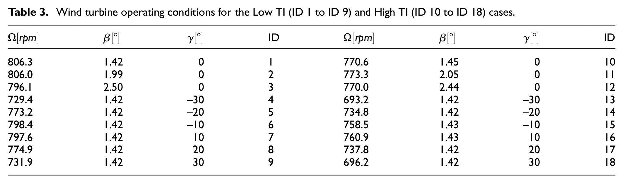
Since the results obtained are almost identical using both the uncoupled and Pitt and Peters (1981) model, the optimization process will be carried out using the Pitt and Peters (1981) correction.

1 × 1 G1 parameters estimation

The LSQ procedure was very effective. This is shown by comparing the initial value of the proposed cost function for the wake speed parameters:

f_{υ el}^{init} = 2.3076

with the final optimized value:

f_{υ el}^{fin} = 1.5691

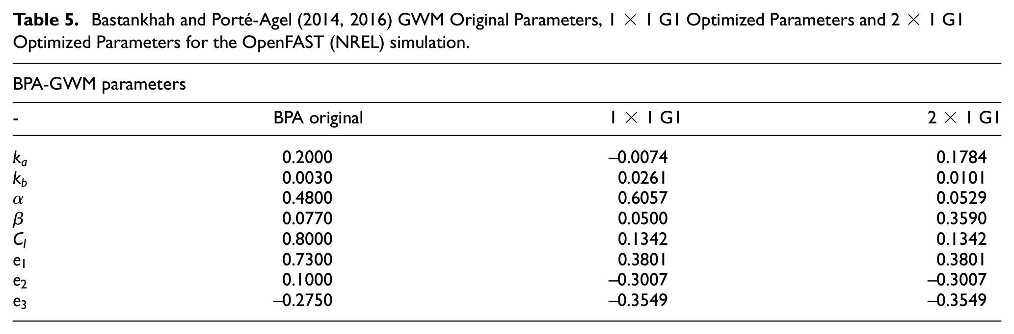
The corresponding set of the velocity and turbulence intensity parameters are:¹ reported in Table 5 under 1 × 1 G1, together with the original ones obtained by Bastankhah and Porté-Agel (2014, 2016).

A reduction of $32 %$ is, thus, observed in the wake velocity cost function and of $88 %$ in the turbulence cost function. The figures reported in Supplemental Material section. Single turbine velocity show the results obtained. It can be seen that in most of the cases, the initial velocity parameters are able to predict the mean velocity quite accurately. However, in some others like the ID1 @ 10D, the discrepancies between the initial and final curves are great. It is interesting to notice how, sometimes, the initial parameters seem to be performing identically (or even better) then the optimized parameter (e.g. in case ID 18 @ 5D). This is due to the fact the optimization is carried out in a “global” way; the overall (and not the local) error is reduced (all the measurements are used for the optimization). From the figures it can be understood that the model accurately predicts the mean velocity up to a yaw angle of approximately 20°. At 30°, the predicted velocity and the experimental one start to differ significantly. This issue was already discussed in the GWM proposed by Bastankhah and Porté-Agel (2014, 2016) and it is one the main limitations of the model.

The figures regarding the turbulence have been obtained optimizing only the non-yawed cases, since the wake width and deflection are already considered in the velocity model. In this case the optimization process has a much greater effect with respect to the initial prediction (the original parameters seem to over-estimate the turbulence intensity in the cases at hand).

2 × 1 G1 Turbine

In the case of the 2 × 1 wind farm, the LSQ procedure becomes much more complex. The number of parameters to be optimized remains the same (a total of eight), but in this case the wake velocity and added TI parameters are coupled. To be rigorous, the whole eight parameters should be optimized altogether due to their influence over each other. However, to simplify the procedure (that otherwise would be very computationally expensive and not guaranteed to succeed) the same hypothesis made in the single turbine case was done. So, the wake model parameters are optimized separately with respect to the added TI parameters.

At the beginning of the optimization, the added TI parameters obtained in the case of a single turbine were used. After the velocity coefficients LSQ procedure is carried out, the added TI parameters will be optimized and compared to the ones relative to the single turbine case (so as to verify eventual discrepancies). A further difference in the optimization process of the 2 × 1 wind farm, with respect to the single turbine case, is the logic with which the optimization is done. In this case, when varying the GWM parameters toward the optimal solution, the $C_{T}$ and the rotor averaged $AIF$ of the G1 turbine downstream change. So, for every optimization step, it is necessary to run a new OpenFAST (NREL) simulation with the newly evaluated OpenFAST (NREL) parameters (this process has been completely automatized) in order to proceed with the minimization. Table 4 summarizes the experimental data used for the GWM optimization.

Table 4.

Wind turbines operating conditions for the Low TI (ID 1 to ID 9) and High TI (ID 10 to ID 18) cases.

$Ω_{1} [rpm]$	$Ω_{2} [rpm]$	$β_{1} [°]$	$β_{2} [°]$	$γ_{1} [°]$	$γ_{2} [°]$	$C T_{1}$	$C T_{2}$	$ID$
816.50	561.71	0.43	0.42	0	0	0.88	0.92	1
746.39	702.00	0.42	0.42	30	0	0.63	0.88	2
746.89	615.42	0.42	0.42	30	30	0.63	0.64	3
812.09	521.77	0.43	0.42	0	30	0.88	0.67	4
817.52	570.41	1.23	0.42	0	0	0.81	0.92	5
806.20	578.58	1.78	0.42	0	0	0.76	0.92	6
813.21	547.86	1.08	2.19	0	0	0.83	0.77	7
805.66	558.02	1.80	2.02	0	0	0.76	0.78	8
780.06	608.03	0.46	0.42	0	0	0.87	0.91	9
714.10	685.29	0.42	0.42	30	0	0.62	0.87	10
715.85	610.26	0.42	0.42	30	30	0.63	0.64	11
784.20	555.81	0.49	0.42	0	30	0.86	0.66	12
784.18	618.43	1.42	0.42	0	0	0.80	0.91	13
777.66	623.91	1.85	0.42	0	0	0.76	0.91	14
784.55	603.06	1.42	1.71	0	0	0.80	0.79	15
779.28	609.36	1.91	1.78	0	0	0.75	0.79	16

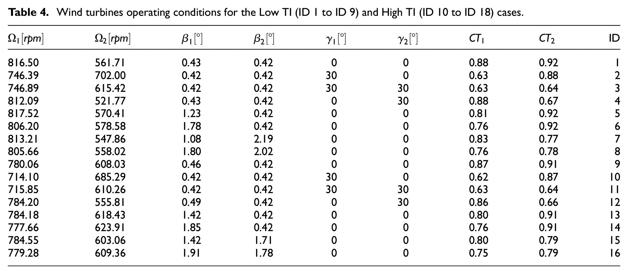
Only the measurements at $10 D$ downwind the first turbine have been considered. Indeed, the measurements at $7.5 D$ were in the near wake region of the downstream turbine (according to the GWM model).

2 × 1 G1 parameters estimation

The values of the initial and final cost function are:

\begin{matrix} f_{υ el}^{init} = 2.6164 \\ f_{υ el}^{fin} = 1.1697 (= f_{υ el}^{init} - 55 % f_{υ el}^{init}) \end{matrix}

The parameter’s value obtained can be found in Table 5 under 2 × 1 G1, together with the optimized 1 × 1 G1 case and the original ones proposed by Bastankhah and Porté-Agel (2014, 2016).

Table 5.

Bastankhah and Porté-Agel (2014, 2016) GWM Original Parameters, 1 × 1 G1 Optimized Parameters and 2 × 1 G1 Optimized Parameters for the OpenFAST (NREL) simulation.

BPA-GWM parameters
-	BPA original	1 × 1 G1	2 × 1 G1
$k_{a}$	0.2000	−0.0074	0.1784
$k_{b}$	0.0030	0.0261	0.0101
$α$	0.4800	0.6057	0.0529
$β$	0.0770	0.0500	0.3590
$C_{I}$	0.8000	0.1342	0.1342
$e_{1}$	0.7300	0.3801	0.3801
$e_{2}$	0.1000	−0.3007	−0.3007
$e_{3}$	−0.2750	−0.3549	−0.3549

The figures reported in Supplemental Material section. Wind Farm velocity show the experimental velocity and the velocity predicted by the model both using the initial parameters (the optimized parameters obtained for the case of a single turbine) and the optimized parameters. It can be seen that the initial model (single turbine optimal parameters) gives poor results when partial wake superimposition happens (downstream the second turbine). At the opposite, the optimization process gives good results when both turbines are not yawed and when only the downstream turbine is yawed. When both turbines have a yaw angle of 30°, the model is able to accurately predict the minimum velocity but not the wake deflection. This is a confirmation of the limitations of the model. The results are quite poor also in the case where only the upstream turbine is yawed. Here, the model cannot predict both the wake deflection and the minimum velocity.

In order to validate the implemented model, simulations have also been performed using the classic FLORIS (NREL). The results are plotted in the same figures of Supplemental Material section. Wind Farm velocity. FLORIS (NREL) and OpenFAST (NREL)/GWM results are similar both in the case where the predicted values are close to the experimental data and in the case where they are not. This suggests that different corrections are needed if the model is intended to be used when the wakes are partially overlapping (the cases where the yaw angles of the first and second turbine differ significantly).

Since the optimization process hasn’t taken into account the turbulence, an a-posteriori check has been performed. This was necessary to see if the parameters computed in the case of the single turbine are acceptable also for the two-turbines case as well. In Supplemental Material section. Wind Farm turbulence intensity, figures showing the experimental turbulence intensity at 10D downstream the first turbine are reported. In the figures it is reported also the average turbulence intensity that would be seen from a hypothetical turbine having zero yaw angle placed at 10D from the downstream turbine. As can be seen, the model already accurately predicts the turbulence level in the region where the two wakes are superimposed. Hence, no further investigation was deemed necessary.

A comparison with literature GWM parameters

It is interesting to compare the parameters obtained in the current LSQ procedure with the ones originally proposed by Bastankhah and Porté-Agel (2014, 2016) reported in Table 5. It is found, by comparison with the experimental data gathered in the wind tunnel, that the GWM with the original parameters is in good agreement with the optimized parameters in some conditions, while in others the error is relevant. However, also in the optimized case, there are some limit conditions in which the GWM is not performing exceptionally. This consideration leads to the idea that, to further increase the modeling capabilities of the GWM, a new formulation could be produced where the parameters to be optimized are no more constant. Instead, they could present some kind of relation to external environmental conditions (i.e.: wind speed, TI, etc. …) or to some control variables (like the yaw of the turbine, the pitch of the blades, etc. …). Overall, the optimized parameters are found to be performing better in almost all the operating conditions for which the GWM is intended to be used. The operating conditions for which the model is intended to be used have been specified in great detail in the previous work of Bastankhah and Porté-Agel (2016, 2014). Here we report briefly the main requirements for the model to be valid: yaw angle values up to 20°, thrust coefficient $C_{T} < 0.96$ (turbine working in windmill state) and the requirement that the turbines composing the wind farm should be working in the far wake zone (the current model doesn’t account for the pitch angle of the blades, if not by means of the thrust coefficient $C_{T}$ ).

Results and discussion

In this section, the results obtained from the validation procedure will be presented. The focus will be on trying to derive some meaningful physical considerations from the parameters obtained during the LSQ Minimization procedure.

It has been shown that the OpenFAST (NREL)/GWM’s results match the experimental data recorded for the single turbine case when the turbine is working at yaw angles up to 20°. After this yaw value, the results start to differ from the experimental data. Thus, the model output can or cannot be useful depending on the application chosen. For the wind farm configuration, the model instead gives poor results in the case where the upstream turbine has a yaw angle of 30° and the downstream turbine has a zero yaw angle. The cause of this problem might be due to the well-known secondary steering effect (not captured by the model) or by other model limits (i.e.: the quadratically added turbulence intensity might not be sufficient or parameters depending on the working conditions of each wind turbine might be needed). From the comparison with the original GWM, it can be stated that the problems encountered in the GWM coupled to OpenFAST (NREL)are also present in FLORIS (NREL), thus a modification of the wake superimposition models is necessary to overcome the issue. It should also be noticed that the results of the proposed version of the GWM and the original Bastankhah and Porté-Agel (2014, 2016) version, in terms of wake velocity, are comparable because all the simulations have been performed in steady-state conditions. Greater discrepancies between the results of OpenFAST (NREL)/GWM and those of FLORIS (NREL) are expected when proper dynamic simulations will be carried out. Once again, it has to be remembered that the GWM is classified as a low-fidelity model. Nonetheless, the results in terms of accuracy are quite striking. Of course, if the aim was that of obtaining the closest agreement with experimental data, an higher fidelity model had to be used (like OpenFAST (NREL) and OpenFOAM (2020)/SOWFA (NREL)), but also in this case a correct tuning of the parameters is fundamental. It has to be pointed out that the number of parameters in a CFD coupled simulation (like OpenFAST (NREL) and OpenFOAM (2020)/SOWFA (NREL)) is incredibly high and that finding the best values for them could be a much difficult problem than the one faced for the GWM validation.

Conclusions and future works

In this paper, a model based on the Bastankhah and Porté-Agel (2016, 2014) GWM and coupled to the OpenFAST (NREL) framework is validated against experimental data gathered in the context of the European CL-Windcon (2020) experimental campaign. A theoretical explanation of the model, together with its implementation in OpenFAST (NREL) is given. The Wind Tunnel and Numerical setups employed are presented. Finally, the cost functions and the methodology followed to validate OpenFAST (NREL)/GWM are reported, together with a discussion of the results obtained.

For what regards the OpenFAST (NREL)/GWM model, it has to be pointed out that the simulation speed of this could further be increased if all the OpenFAST (NREL) instances (each one representing a single turbine) were run in parallel fashion; however, this would mean rethinking and rewriting the whole InflowWind user-specified routine. Since the implemented model is a steady-state model, this new tool could not be used in order to simulate dynamic or transient conditions. As of today, this is the major drawback of the model, together with the impossibility of reproducing adequately the wake meandering phenomenon and the secondary steering effect that have quite a big impact on the flow field developed inside a wind farm.

In the future the intention is to increase the fidelity of the validated GWM model by adding the capability of representing a dynamic flow condition. However, since the GWM is intended to be used for practical engineering purposes, a lot of effort will be devoted to keeping its formulation computationally cheap and to retain the number of parameters to the smallest possible, while keeping a good accuracy. For the new dynamic GWM, a validation procedure will be needed too. The methods used will be the same adapted in this paper in order to have an equal comparison between the steady-state and the dynamic case.

Thanks to the current work that is now being carried out at Politecnico di Milano, it will be soon possible to validate the OpenFAST (NREL)/GWM model based not only on the experimental data gathered, as done in this work, but also following a completely numerical-based approach that uses CFD methods. Specifically OpenFAST (NREL) and OpenFOAM (2020)/SOWFA (NREL) will be used to reproduce the same wind tunnel tests whose measurements have been used in these paper to perform the validation.

Supplemental Material

sj-pdf-1-wie-10.1177_0309524X221117820 – Supplemental material for Parameters estimation of asteady-state wind farm wake model implemented in OpenFAST

Supplemental material, sj-pdf-1-wie-10.1177_0309524X221117820 for Parameters estimation of asteady-state wind farm wake model implemented in OpenFAST by Antonio Cioffi, Ali Raza Asghar and Paolo Schito in Wind Engineering

Footnotes

Acknowledgements

Thanks to the National Renewable Energy Laboratory (NREL) for the open-source software that have been used in this work.

Declaration of conflicting interests

The author(s) declared no potential conflicts of interest with respect to the research, authorship, and/or publication of this article.

Funding

The author(s) received no financial support for the research, authorship, and/or publication of this article.

ORCID iD

Antonio Cioffi

Supplemental material

Supplemental material for this article is available online.

Notes

References

Barthelmie

Hansen

Frandsen

, et al. (2009) Modelling and measuring flow and wind turbine wakes in large wind farms offshore. Wind Energy 12(5): 431–444.

Bastankhah

Porté-Agel

(2014) A new analytical model for wind-turbine wakes. Renewable Energy 70: 116–123.

Bastankhah

Porté-Agel

(2016) Experimental and theoretical study of wind turbine wakes in yawed conditions. Journal of Fluid Mechanics 806: 506–541.

Bay

King

Fleming

, et al. (2019) Unlocking the full potential of wake steering: Implementation and assessment of a controls-oriented model. Wind Energy Science Discussions 1–20. DOI:10.5194/wes-2019-19.

Campagnolo

Molder

Schreiber

, et al. (2019) Comparison of analytical wake models with wind tunnel data. Journal of Physics Conference Series 1256: 012006.

Cioffi

Muscari

Schito

, et al. (2020) A steady-state wind farm wake model implemented in openfast. Energies 13(23): 6158.

CL-Windcon (2020) Cl-Windcon. Available at: http://www.clwindcon.eu/public-deliverables/ (accessed 18 December 2020).

Crespo

Hernandez

(1996) Turbulence characteristics in wind-turbine wakes. Journal of Wind Engineering and Industrial Aerodynamics 61(1): 71–85.

EN 1991-1-4:2005(E) (2005) Eurocode 1: Actions on Structures - Part 1-4: General Actions - Wind Actions. Bruxelles: Standard, European Committee for Standardization.

10.

Farrell

King

Draxl

, et al. (2021) Design and analysis of a wake model for spatially heterogeneous flow. Wind Energy Science 6(3): 737–758.

11.

FloriDyn (Becker) (2020) Floridyn. Available at: https://github.com/MarcusBecker-GitHub/FLORIDyn_Matlab (accessed 16 January 2021).

12.

FLORIS (NREL) (2020) Floris. version 2.2.0. Available at: https://github.com/NREL/floris (accessed 2 December 2020).

13.

Frandsen

Barthelmie

Pryor

, et al. (2006) Analytical modelling of wind speed deficit in large offshore wind farms. Wind Energy 9(1–2): 39–53.

14.

Gebraad

PMO

Teeuwisse

van Wingerden

, et al. (2014) A data-driven model for wind plant power optimization by yaw control. In: 2014 American Control Conference. pp. 3128–3134. DOI:10.1109/ACC.2014.6859118.

15.

Gebraad

PMO

Teeuwisse

van Wingerden

, et al. (2016) Wind plant power optimization through yaw control using a parametric model for wake effectsa cfd simulation study. Wind Energy 19: 95–114.

16.

Gebraad

PMO

van Wingerden

(2014) A control-oriented dynamic model for wakes in wind plants. Journal of Physics Conference Series 524: 012186.

17.

Jensen

(1983) A Note on Wind Generator Interaction. Number 2411 in Risø-M. Roskilde: Risø National Laboratory.

18.

Katic

Højstrup

Jensen

(1987) A simple model for cluster efficiency. In: EWEC’86. Proceedings (eds Palz

Sesto

), vol. 1, pp.407–410. A. Raguzzi.

19.

Lagarias

Reeds

Wright

, et al. (1998) Convergence properties of the Nelder-Mead simplex method in low dimensions. SIAM Journal on Optimization 9: 112–147.

20.

Larsen

Aagaard

Bingöl

, et al. (2007) Dynamic Wake Meandering Modeling. Denmark: Forskningscenter Risoe.

21.

Niayifar

Porté-Agel

(2015) A new analytical model for wind farm power prediction. Journal of Physics Conference Series 625: 012039.

22.

OpenFAST (NREL) (2020) Openfast. Available at: https://github.com/OpenFAST/openfast. (accessed 2 December 2020).

23.

OpenFOAM (2020) Openfoam. Available at: http://www.openfoam.org. (accessed 2 December 2020).

24.

Pitt

Peters

(1981) Theoretical prediction of dynamic-inflow derivatives. Vertica 5(1): 21–34.

25.

Porté-Agel

Chen

(2013) A numerical study of the effects of wind direction on turbine wakes and power losses in a large wind farm. Energies 6(10): 5297–5313.

26.

Schito

Zasso

(2014) Actuator forces in cfd: Rans and les modeling in openfoam. Journal of Physics Conference Series 524: 012160.

27.

SOWFA (NREL) (2020) Sowfa. Available at: https://github.com/NREL/SOWFA. (accessed 2 December 2020).

28.

Srensen

(2012) 2.08 - aerodynamic analysis of wind turbines. In: Sayigh

(ed.) Comprehensive Renewable Energy. Oxford: Elsevier, pp.225–241.

29.

van Dijk

van Wingerden

Ashuri

, et al. (2017) Wind farm multi-objective wake redirection for optimizing power production and loads. Energy 121: 561–569.

30.

Vermeer

Sørensen

Crespo

(2003) Wind turbine wake aerodynamics. Progress in Aerospace Sciences 39(6-7): 467–510.

Supplementary Material

Please find the following supplemental material available below.

For Open Access articles published under a Creative Commons License, all supplemental material carries the same license as the article it is associated with.

For non-Open Access articles published, all supplemental material carries a non-exclusive license, and permission requests for re-use of supplemental material or any part of supplemental material shall be sent directly to the copyright owner as specified in the copyright notice associated with the article.

0.00 MB

4.63 MB