Analysis for the prediction of solar and wind generation in India using ARIMA,linear regression and random forest algorithms

Abstract

This work focused on the prediction of generation of renewable energy (solar and wind) using the machine learning ML algorithms. Prediction of generation are very important to design the better microgrids storage. The various ML algorithms are as logistic regression LR and random forest RA and the ARIMA, time series algorithms. The performance of each algorithm is evaluated using the mean absolute error, mean squared error, root mean squared error, and mean absolute percentage error. The MAE value for the ARIMA (0.06 and 0.20) model for solar and wind energy is very less as compared to RF (15.65 and 61.73) and LR (15.78 and 54.65) of solar and wind energy. Same with MSE and RMSE, the MSE and RMSE value for the ARIMA of solar energy model obtained is 0.01 and 0.08 and wind energy is 0.07 and 0.27 respectively. Comparative analysis of all of these matrices of each algorithm for both the dataset, we concluded that the ARIMA model is best fit for the forecasting of solar energy and wind energy.

Keywords

Renewable energy solar energy wind energy machine learning linear regression random forest time series ARIMA MAE MSE RMSE MAPE

Introduction

Electricity is generated from a variety of sources, including hydropower, nuclear power, and renewable energy. Coal, oil, or natural gas are used to produce power, account for 1/3rd of global greenhouse gas productions. It is vital to raise citizens’ quality of life by supplying clean and efficient electricity. To achieve the country’s economic development goals, India’s energy demand is increasing A growing supply of energy is a basic requirement for a nation’s economic success. The National Electricity Plan of the Ministry of Power has created a 10-year plan of action with the purpose of offering power across the nation, and also provide an idea to ensure that power is supplied to residents efficiently and at an affordable price. In this way, the govt will accelerate and globalize the transition to RE technology in order to attain imperishable development. Renewable energy can be considered as having capacity to reach the demand of power and also minimize the pollution (Ahmad et al., 2020; Alkandari and Ahmad, 2020; Ikram, 2021).

To save energy residents have motivated to use wind, solar as these are inexhaustible in nature. It goes without saying that sustainable energy is fewer costlier and hazardous. India has an aim of achieving 175 GW energy from renewable by 2022. Solar accounting for 100 GW, 10, 60 and 5 GW accounts for biomass, wind and hydro respectively. Renewable energy comes from natural processes that are renewed on a regular basis. The majority of renewable energy sources are environmentally beneficial and help to reduce carbon emissions, which in turn helps to battle global warming.

Renewable energy is seen as the most encouraging replacement of fossil fuel since it is clean, green, and regenerated over a large geographic region; yet, it also introduces unplanned uncertainty, endangering energy reliability and stability, particularly when it comes to large-scale renewable energy integration (Qiao, 2019). In the latest decades, the electricity market has moved its attention to renewable energy sources to minimize its greenhouse discharge during power production. Solar and wind have regularly been used as a combination due to their RE variety and reliability. Several approaches for predicting RE have been grown over time, all of which have emphasized on the efficiency of estimation techniques with no or small concern for the environmental conditions. Renewable energy can efficiently cut fossil energy use, minimize pollution, and promote the healthy growth of the social economy (Fathollahzadeh et al., 2021; Jia et al., 2021).

Due to the variable character of power production from solar and wind, the operators must regulate and maintain power system properly. The electricity production of photovoltaic-wind must be forecasted to schedule the power transmission for long and short term (Somu et al., 2021). Energy Prediction using Hybrid Renewable Energy Systems proposed. Figure 1 represent classification of generation or power based on time. (Bakhtiari et al., 2021; Lee et al., 2019; Rahman et al., 2021; Somu et al., 2021).

Figure 1.

Horizon and timeframe of prediction.

Solar Energy Prediction: Because of its reliance on a variety of elements such as pressure, temperature, speed of wind etc. solar radiation is most stimulating constraints. As these are unpredictable, the machine learning techniques is used for forecasting (Makade et al., 2019). It is the process of collecting and examining data in order to estimate solar power generation across a period of time with an aim of reducing solar intermittency’s impact (Liu et al., 2020). Solar power forecasting is used to operate the electric grid more efficiently and for power trading (Rahul et al., 2021).

Wind Energy Prediction: For the fluctuated nature of wind, it is necessary to do prediction. Due to fluctuation in speed of wind, forecast is not an easy task. To increase wind prediction efficacy, several ML techniques have been used (Lai et al., 2020). Study based on NARX prediction models in wind-speed forecasting discussed for short-term scheme (Di Piazza et al., 2016). There are various techniques used in machine learning for the prediction such as (Mosavi et al., 2019)

LR: Linear Regression

RF: Random Forest

ARIMA: Autoregressive integrated moving average

AR: Autoregressive etc. … Machine learning (ML) approaches are now widely used in a variety of renewable energy-related applications, including the growth of energy and unification, utilization, and forecasting (Hosein et al., 2020). The remaining part of this study is presented as follows: A proposed plan is conducted in Part 2. Study design and methodology is described in Part 3. At last, Part 4 and 5 brings the paper to an end with results and conclusion.

Proposed plan

In this study, for the prediction of Solar and Wind Energy, we are using three machine learning algorithms.

ARIMA

Logistic Regression

Random Forest

After applying these algorithms, we are checking the performance of each algorithms using following matrices:

Mean Absolute Error

Mean Squared Error

Root Mean Squared Error

Mean Absolute Percentage Error

Figure 2 represents Working flow for this study.

Figure 2.

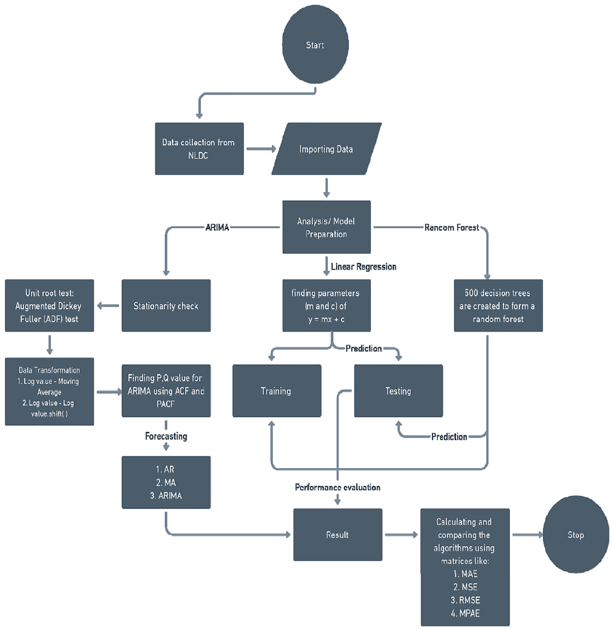
Flowchart for proposed model.

ARIMA

ARIMA is used for time series analysis in which observations are collected in series at specified time intervals. With the help of these series, we can predict the next values on the basis of past data. Generally, in time series, we have only two variables – Time and the feature that we want to forecast. ARIMA is a combination of two models – a. AR (Autoregressive), b. MA (Moving Average)

ARIMA has three hyperparameters that need to be optimized in order to achieve better performance.

(i) p (Autoregressive lags),

(ii) d (Order of differentiating),

(iii) q (Moving Average lags)

Before applying any time series model, stationarity of data is evaluated. Stationary means that over different period of time data should have –

(i) Constant mean, (ii) Constant variance and standard deviation, (iii) Auto-covariance.

Linear regression (LR)

Linear regression is used to predict the value based on some input features. Training is done at the beginning with input and output features. Linear regression is of two types.

Simple linear regression

In this case, only one input feature is taken into consideration with one output variable.

y_{i} = m x_{i} + C

(1)

Where,

$y_{i}$ is the output variable of the $i^{th}$ input

m is the parameter that need to be optimized in order to find best fit line

$x_{i}$ is the $i^{th}$ input of the column x

C is the bias that need to be optimized in order to find best fit line.

Multiple linear regression (MLR)

It has multiple input variables with one output variable. The equation for multi regression is:

y_{i} = a {x_{i}}^{1} + b {x_{i}}^{2} + c {x_{i}}^{3} + . . . + C

(2)

$y_{i}$ is the output variable of the $i^{th}$ input

a, b, c… are the parameter that need to be optimized in order to find best fit line

$x_{i}$ ¹, $x_{i}$ ², $x_{i}$ ³ are the $i^{th}$ inputs of the column x₁, x₂, and x₃ respectively.

C is the bias that need to be optimized in order to find best fit line.

Random forest

It builds decision trees based upon the samples in classification. One of the key features of this algorithm has to be the ability of handling data sets having continuous variables for the cases of regression and categorical variables for classification. Having said that, this algorithm gives better results for classification problems as compared to regression (Liaw and Wiener, 2002).

To be able to understand the working of random forest methods, a concept called the ensemble technique should be known. Ensemble utilizes two types of methods:

Bagging: As mentioned above, a different training subset is generated from the sample training data and majority voting determines the final output data. Random forest uses this method for classification.

Boosting: In this method of ensemble, the final model created gives the maximum accuracy. This is done by generating a sequential model upon combining weak learners with strong learners. Examples of this include ADA BOOST, XGBOOST.

Mean absolute error

MAE is used for measuring the absolute error difference between predicted values and actual values.

Absolute error equation:

E (error) = | x_{predicted} - x_{actual} |

(3)

Mean absolute error equation:

MAE = \frac{1}{n} \sum_{i = 1}^{n} | x_{i}^{predicted} - x_{i}^{actual} |

(4)

Where:

∑ is the summation notation, n is the total number of observations, $x_{i}^{predicted}$ is the value of prediction of $i^{th}$ observation and $x_{i}^{actual}$ is true value of $i^{th}$ observation.

Mean squared error

MSE is a statistical method used to find the squared error between predicted values and actual values. Less the value of MSE, better will be the performance of the machine learning model.

MSE = \frac{1}{n} \sum_{i = 1}^{n} {(x_{i}^{predicted} - x_{i}^{actual})}^{2}

(5)

Root mean squared error

If the value of RMSE is less, then the performance of machine learning will be better.

RMSE = \sqrt{\frac{1}{n} \sum_{i = 1}^{n} (x_{i}^{predicted} - x_{i}^{actual}) 2}

(6)

Mean absolute percentage error

MAPE is used to calculate the performance of machine learning algorithms but instead of accuracy, it measures the accuracy percentage of machine learning algorithms.

Equation for MAPE is:

MAPE = \frac{1}{n} | \frac{x_{i}^{predicted} - x_{i}^{actual}}{x_{i}^{actual}} |

(7)

Study design and methodology

(i) Data collection – For this study, we have collected solar and wind energy generation data in MU (million units) on a daily basis from the National Load Dispatch Centre. Total 1912 observations are collected for both solar and wind energy generation starting from 2017-01-01 to 2022-03-27.

(ii) Tools used – Following tools will be used for the implementation of this study: For machine learning implementation, python programing language is used because of its simplicity, compactness and better readability.

Analysis descriptive summary of data

As we can see from the Table 1, the total number of observed values for both the data is 1912. The maximum unit energy generated for solar energy is 266 MU while for wind energy is 541 MU. Standard deviation of solar energy is 55.19 while for wind is 100.66, that is, there is much variance in wind data so it would be difficult for machine learning algorithms to perform well for wind data.

Table 1.

Descriptive summary of solar and wind energy generation.

SN	Energy	Count	Mean	Std	Min	25%	50%	75%	Max
1	Solar	1912	117.7	55.19	19	77	116.5	157.2	266
2	Wind	1912	151.6	100.6	5.0	80.7	114	207	541

Figures 3 and 4. shows the rolling mean and rolling standard deviation of solar energy and wind energy generation. Both rolling mean and standard deviation are changing over time for solar energy, that is, they are not constant therefore, the solar energy are non-stationary in nature, that is, the values of solar energy generation are changing with time. However, the wind generation data looks somewhat non-stationary in nature.

Figure 3.

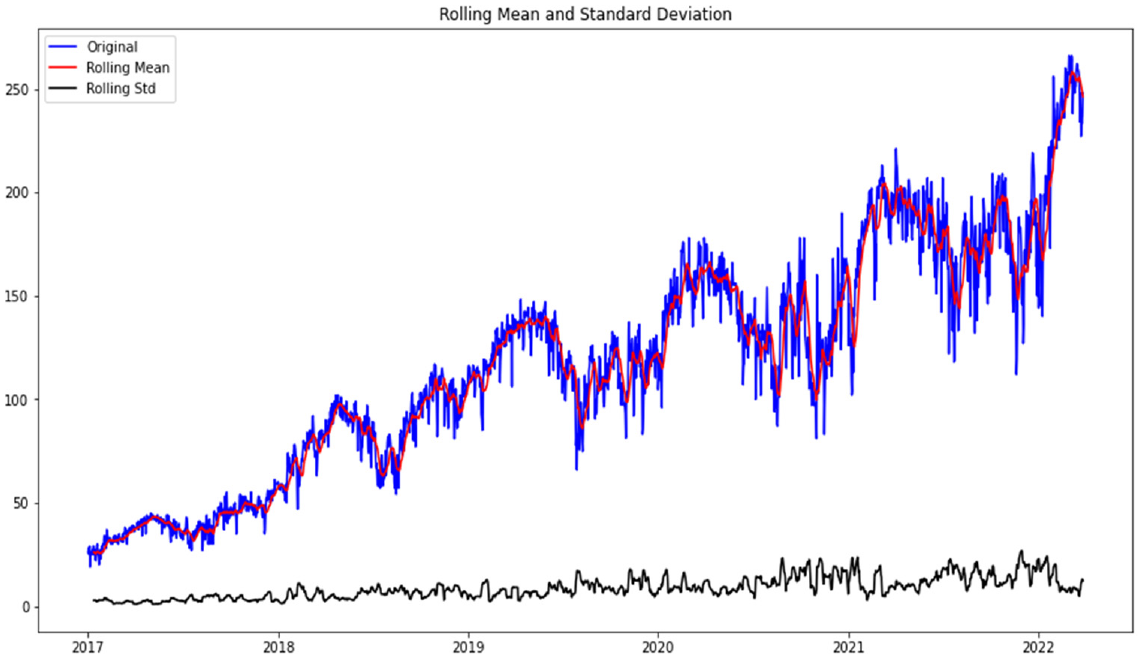
Rolling mean and standard deviation of solar energy generation (MU).

Figure 4.

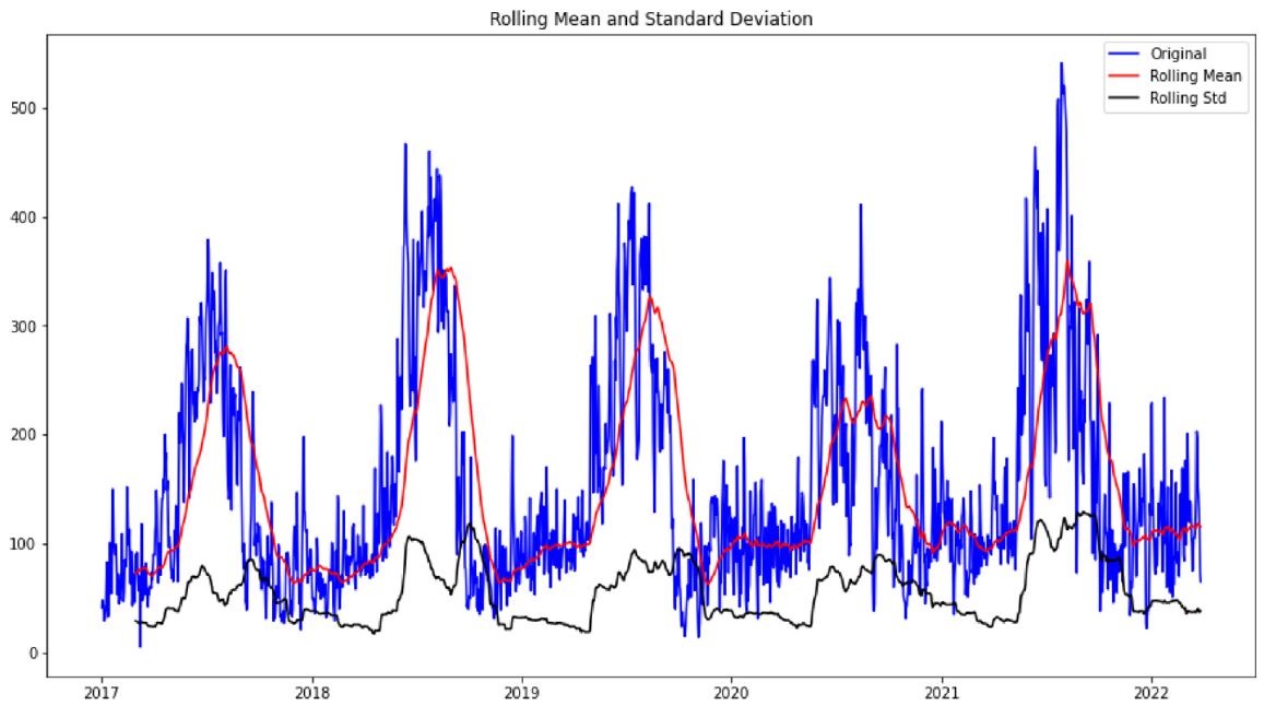
Rolling mean and standard deviation of wind energy generation (MU).

Data transformation to achieve stationarity

To make the data stationary, first we’ll take the log of our data then we will use a differencing method to achieve stationarity. For the accuracy purpose, we will take logarithmic values for wind data as well even though it is already stationary. To make this stationary, we will use a differencing method in which we will take the difference between the log values and moving average values of solar energy generation and wind energy generation.

Log scale(L) = stationary part(L1) + trend (LT)

moving avg of log scale(A) = stationary part (A1) + trend (AT)

result series (R) = L − A = (L1 + LT) − (A1 + AT) = (L1 − A1) + (LT − AT)

Now, both log scale(L) and moving av of log scale(A) is part of series and moving average therefore, the trend will be almost the same, that is, LT - AT = 0 and trend component will be almost removed.

R = L1 – A1

Following graphs (Figures 5 and 6) shows the representation of each energy after removal of trend.

Figure 5.

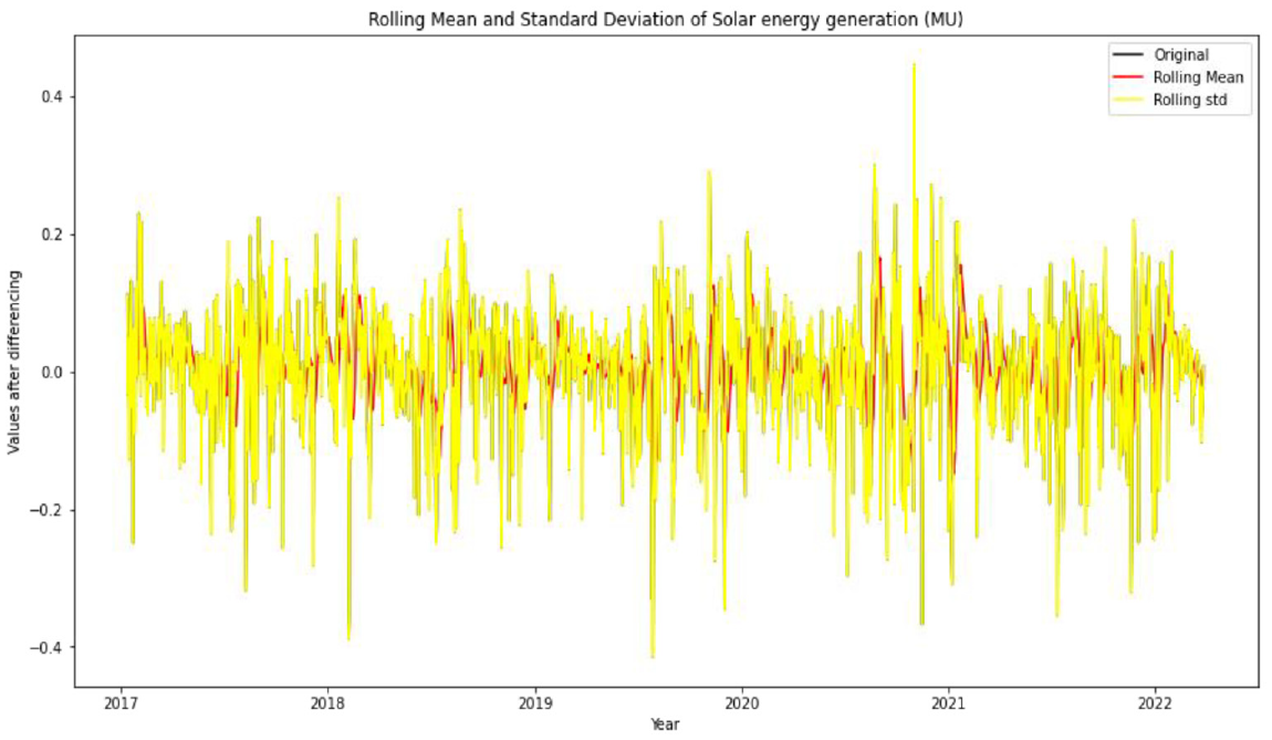
Rolling mean and standard deviation of solar energy generation (MU).

Figure 6.

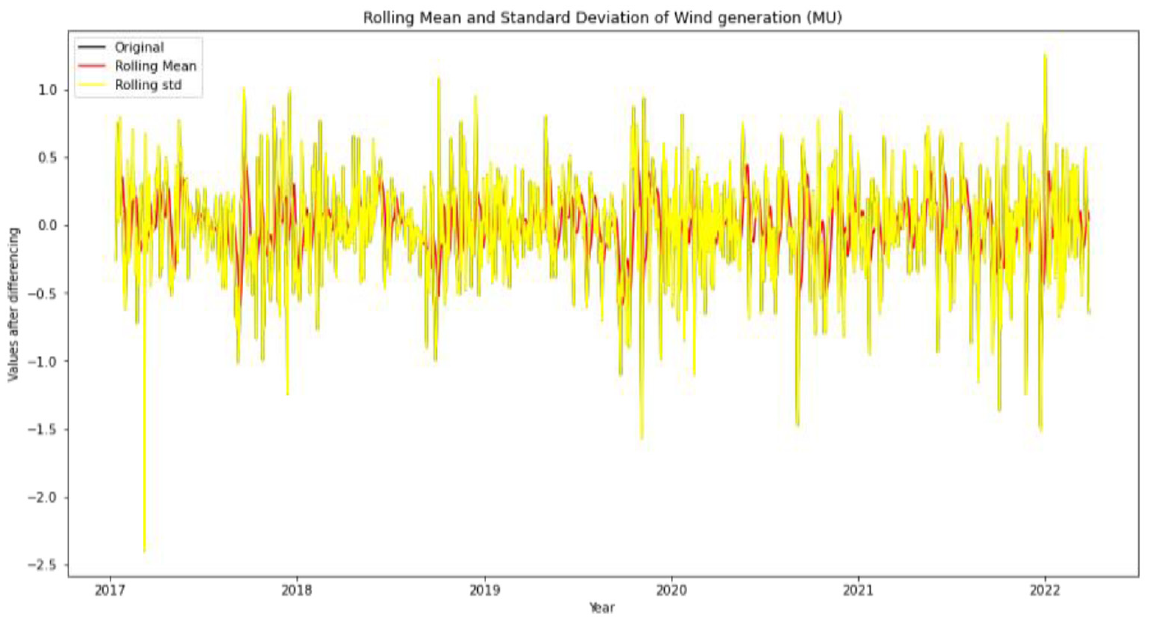
Rolling mean and standard of wind energy generation (MU).

Black line of above graphs represents the original value, that is, result series (r) which is L1 – A1. Above graph seems stationary in nature that is, their mean and standard deviation after some interval is almost same as any particular interval.

Building time series model

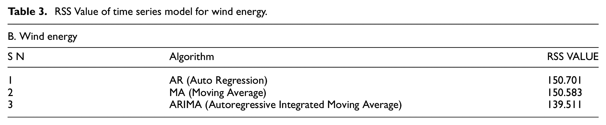
In this study, we are using time series models like AR, MA, and ARIMA for forecasting the solar and wind energy generation 1 year ahead in future. Thus, to get the better model, we will compare all these three models RSS (Residual Sum of Squares) value to get the better model for forecasting the energy generation.

Residual Sum of Squares is used to estimate the variance between the fitted line and the regression function.

RSS = \sum_{i = 1}^{n} (y_{i} - (f (x_{i}))^{2}

(8)

Where:

$y_{i}$ = $i^{th}$ value of variable to be predicted

$f (x_{i})$ = predicted value of $i^{th}$ term

From the Tables 2 and 3, the RSS value of ARIMA is lower than the RSS value of both AR and MA therefore, ARIMA will perform better for forecasting both the solar and wind energy generation as compared to AR and MA.

Table 2.

RSS Value of time series model for solar energy.

A. Solar energy
S N	Algorithm	RSS VALUE
1	AR (Auto Regression)	14.6849
2	MA (Moving Average)	14.069
3	ARIMA (Autoregressive Integrated Moving Average)	13.1328

Table 3.

RSS Value of time series model for wind energy.

B. Wind energy
S N	Algorithm	RSS VALUE
1	AR (Auto Regression)	150.701
2	MA (Moving Average)	150.583
3	ARIMA (Autoregressive Integrated Moving Average)	139.511

Linear regression model

Now that we have prepared our model for the ARIMA model, let’s see how linear regression is working on this problem. For linear regression inputs and outputs, we selected our input as the “Solar energy generation (MU)” and output as Average of “Solar energy generation (MU) after 365 days.” Since, we have only two variables in this problem therefore, this is a simple linear regression problem. The equation for simple linear regression is -

y_{i} = m x_{i} + C

$y_{i}$ is the predicted value of $i^{th}$ value

m is the slope of line that need to be optimized

c is intercept of line that need to be optimized

Solar energy

After fitting the linear regression model to our data, the obtained values of m and c for solar energy are 0.88 and 46.87 respectively. Therefore, the final equation of linear regression for solar energy generation will be-

y_{i} = 0.88 x_{i} + 46.87

Thus, from the above equation, as the value of $x_{i}$ is increasing, the value of $y_{i}$ is also increasing with a rate of 0.88

Wind energy

Similarly, for wind energy generation, the obtained m and c values are 0.704 and 53.49 respectively. Therefore, equation of wind energy generation for linear regression will be –

y_{i} = 0.704 x_{i} + 53.49

Here also the value of $y_{i}$ is increasing as $x_{i}$ increases.

Random forest model

Next, we are using the Random Forest machine learning model.

Random forest is a very popular and powerful machine learning algorithm which works on combination of multiple decision trees. For this study, we are using a combination of 500 decision trees for preparation of a random forest model. One such tree for both solar and wind energy is shown below in Figure 7 .

Figure 7.

Decision tree of Random Forest for first estimator of solar energy.

In the same ways decision tree of Random Forest for first estimator of wind energy Can also presented.

Results and discussion

Visualizations

Now that we have prepared all the algorithms, we are now predicting or forecasting the result of energy generation for 1 year ahead in future. Collected data last date is 2022-03-27 and 1 year prediction, that is, on 2023-03-27, the graph for this prediction is shown below using each algorithm for both the energies generation.

ARIMA

Figure 8 shows the confidence interval of predicted values, that is, the forecasting results will range in shaded regions with the probability of 95%. Figures 8 and 9 represent ARIMA forecast trend of solar and wind energy generation.

Figure 8.

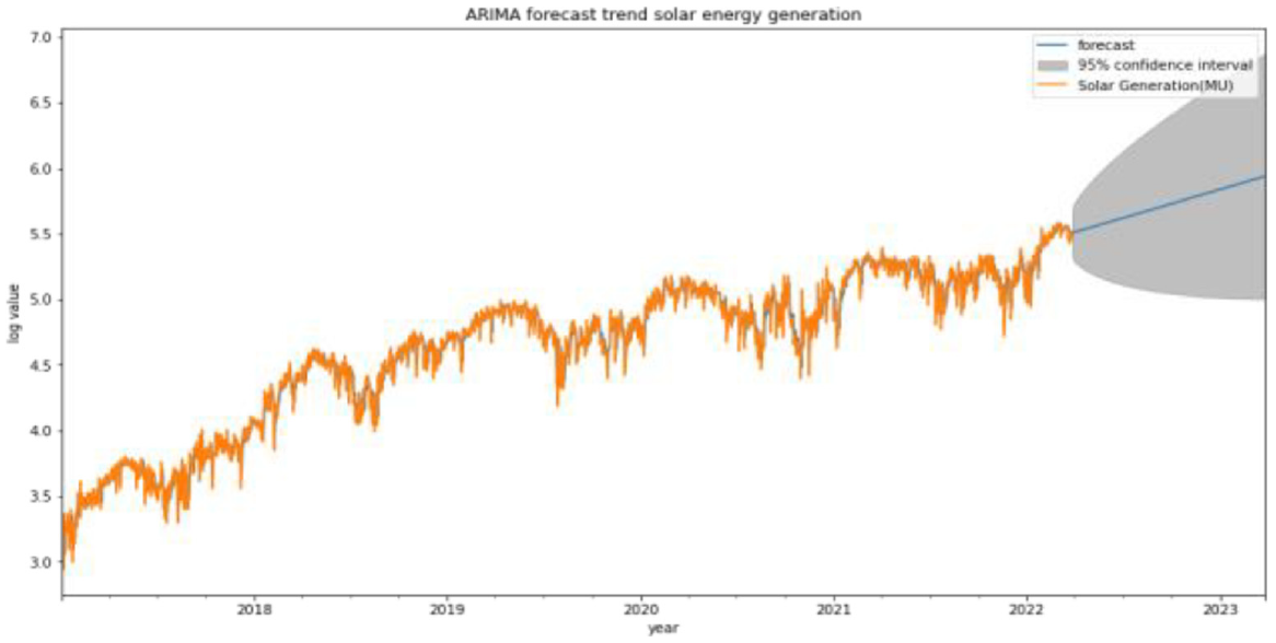
ARIMA forecast trend of solar energy generation.

Figure 9.

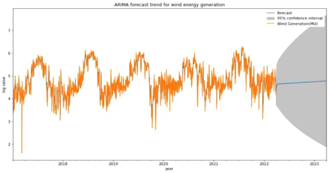
ARIMA forecast trend of wind energy generation.

Random forest

Figure 10 and 11 represents Random forest prediction for solar & wing energy generation.

Figure 10.

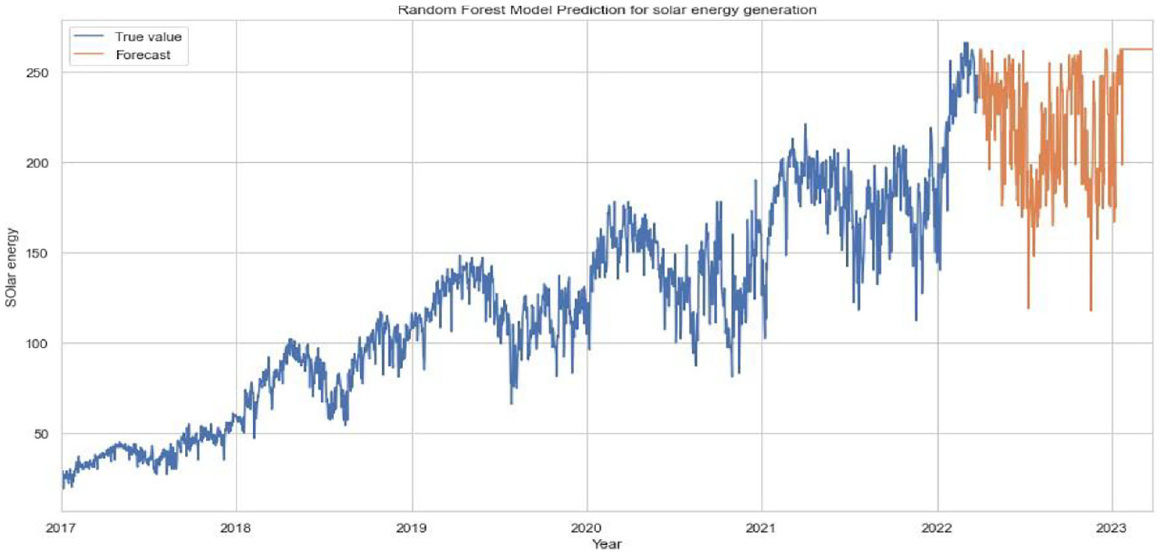
Random forest prediction for solar energy generation.

Figure 11.

Random forest prediction for wind energy generation.

Linear regression

Figures 12 and 13 represent Linear regression model prediction for solar and wind energy generation.

Figure 12.

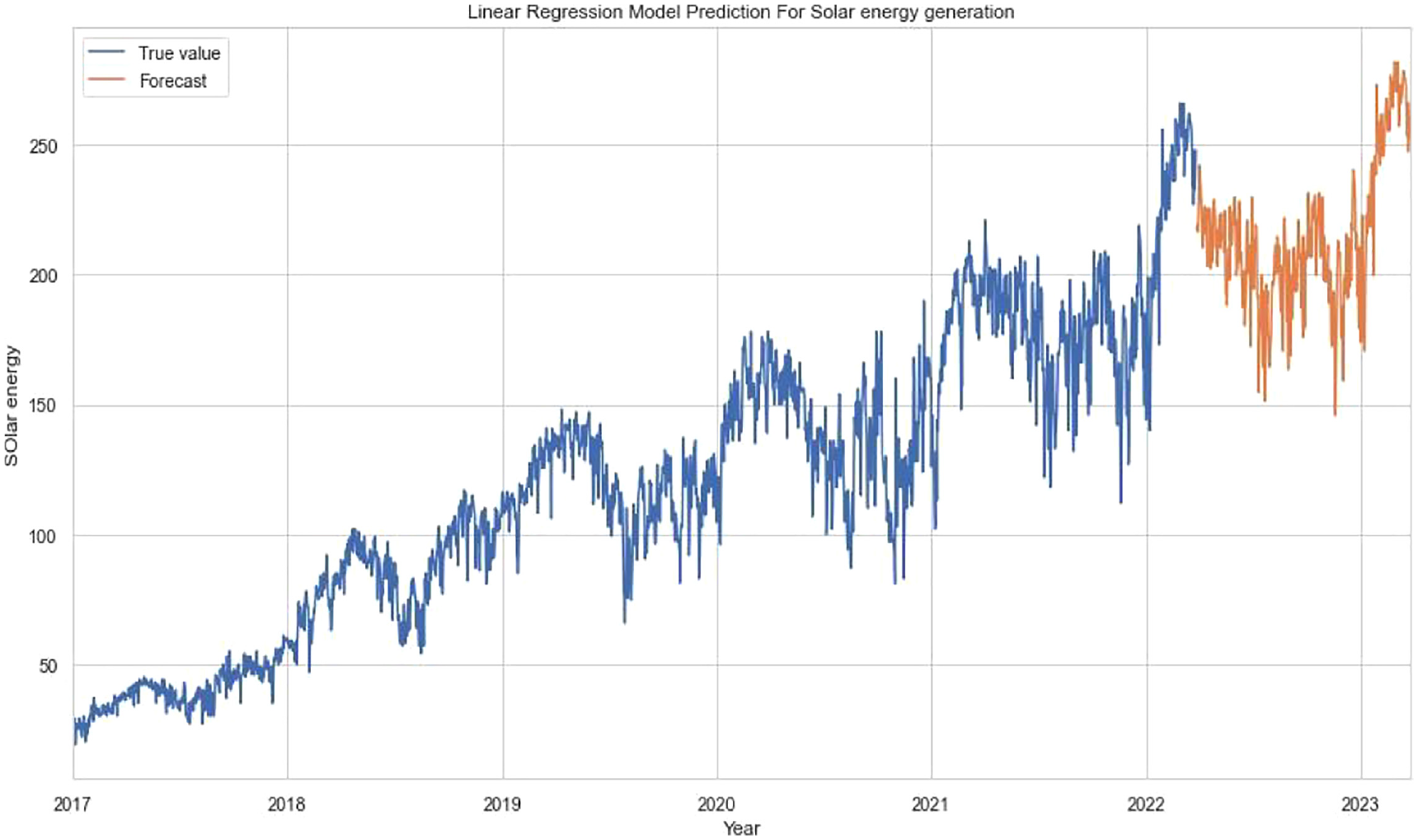
Linear regression model prediction for solar energy generation.

Figure 13.

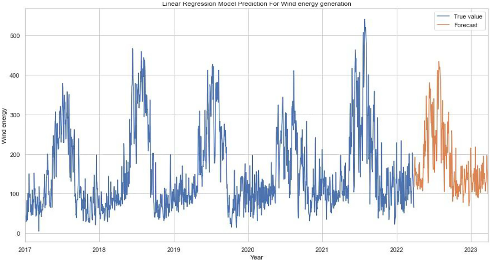
Linear regression model prediction for wind generation.

Prediction results

The value of solar and wind energy generation according to ARIMA, Random Forest and Linear regression on 2022-03-27 is shown in above table (Table 4).

Table 4.

Predicted values, Mean and Std for solar and wind energy using ARIMA, RF, and LR.

S. No.	Date	Energy type	Value	Mean	Count
ARIMA
1.	2023-3-27	Solar Energy	379.02	30.98	38.37
2.	2023-3-27	Wind Energy	118.52	110.41	5.45
Random forest
3.	2023-3-27	Solar Energy	262.14	225.44	33.26
4.	2023-3-27	Wind Energy	97.87	175.26	86.69
Linear regression
5.	2023-3-27	Solar Energy	266.32	215.14	28.03
6.	2023-3-27	Wind Energy	99.29	180.31	81.11

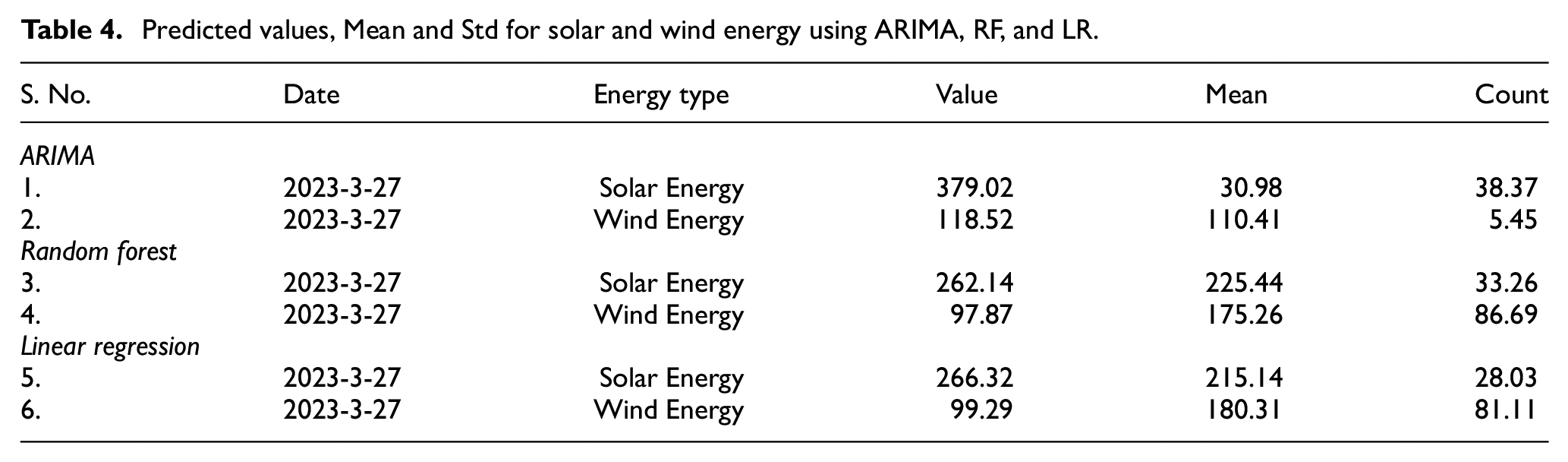
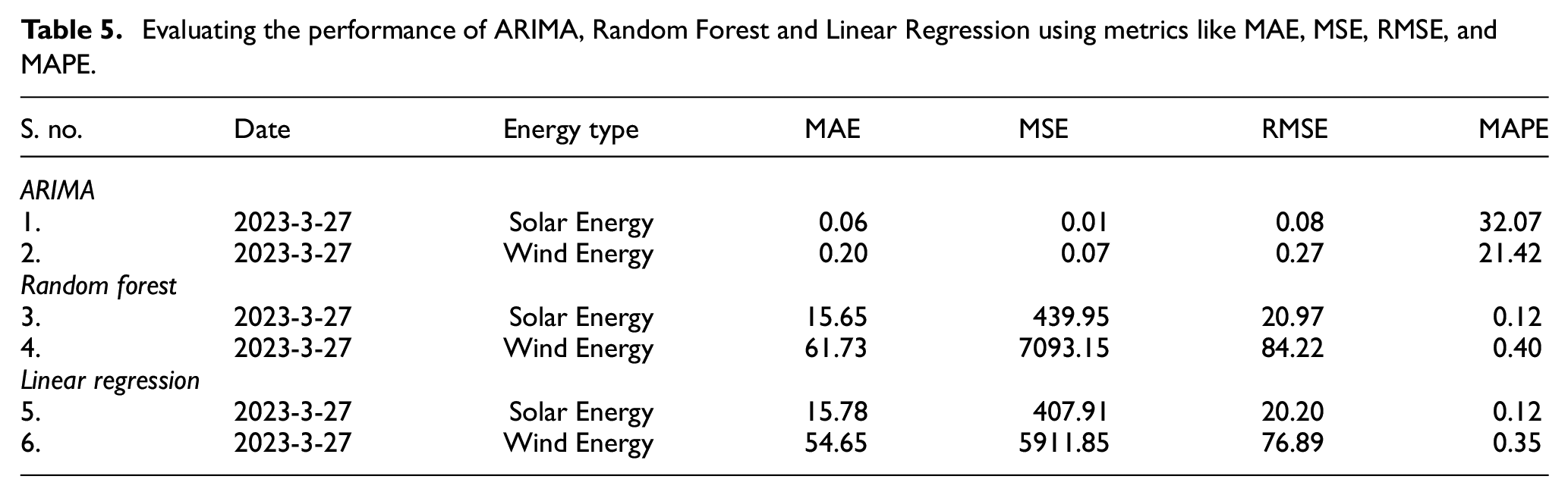
From the above table, we have compared predicted result of each model for both the energies on 2023-03-27. But the values of each model are varying therefore, we have to find the best model for the prediction of solar and wind energy generations. For that we are going to compare all these algorithms by using some useful metrics like MAE, MSE, RMSE, MAPE (Table 5).

Table 5.

Evaluating the performance of ARIMA, Random Forest and Linear Regression using metrics like MAE, MSE, RMSE, and MAPE.

S. no.	Date	Energy type	MAE	MSE	RMSE	MAPE
ARIMA
1.	2023-3-27	Solar Energy	0.06	0.01	0.08	32.07
2.	2023-3-27	Wind Energy	0.20	0.07	0.27	21.42
Random forest
3.	2023-3-27	Solar Energy	15.65	439.95	20.97	0.12
4.	2023-3-27	Wind Energy	61.73	7093.15	84.22	0.40
Linear regression
5.	2023-3-27	Solar Energy	15.78	407.91	20.20	0.12
6.	2023-3-27	Wind Energy	54.65	5911.85	76.89	0.35

Main Model issue is to training of time-series RE data efficiently form the large number of data set and the selection of proper network, applied algorithm for the forecast output. It is changing with the specific dataset.

Data collection

For this study, we have collected solar and wind energy generation data in MU (million units) on a daily basis from the National Load Dispatch Center and GitHub. Total 1912 observations are collected for both solar and wind energy generation starting from 2017-01-01 to 2022-03-27.

Tools used:

Following tools will be used for the implementation of this study: For machine learning implementation, python programing language is used because of its simplicity, compactness and better readability. Python programing language with following libraries of python is used: Sklearn, Pandas, Numpy, Matplotlib, Seaborn, time

Literature analysis

A broad analysis of prediction of RE depending on deep neural network, ANN, FUZZY, LSTM, ARIMA, CNN, Spatio-Temporal Methods, XG Boost Model, LightG, RM, etc techniques are mentioned in a tabular form in Table 6 and additional techniques for investigating its efficacy and applications.

Table 6.

Summary of models and sources used in prediction.

Author	Technique used	Source
Qiao (2019)	Neural Network, BP and NIMF	Wind Energy
Kim et al. (2019)	Random Forest Regression Algorithm	Solar Power
Somu et al. (2021)	Clustering, CNN, LSTM	Electricity
Jana et al. (2020)	MODWT, LSTM	Residential, Commercial, industrial, Transport sectors
Ehsan et al. (2020)	Deep structured Network, CNN, LSTM	Wind Power
Agarwal et al. (2020)	Regression Model	Solar Power
Cao et al. (2021)	RF & GRF model and LSTM Model	Wind Power
Khan et al. (2020)	Category Boosting, MLP, SVR, soft-Computing	Wind Energy, Solar Energy, Non-Renewable Energy
de Jongh et al. (2020)	Spatio- Temporal Methods, LSTM, Auto Regressive-Moving Average (ARMA), Quantile Regression (QR)	Solar Energy
Thukral (2020)	MLFNN, MLR, NN	Solar Power
Long and Zhang (2020)	Ensemble Learning Algorithm, support vector regression,	Wind Energy
Ahmad et al. (2020)	Artificial Neural Networks (ANN), Ensemble Models	Wind, Solar, and Geothermal Energy,and Electricity
Cao et al. (2021)	Deep Recurrent type-three Fuzzy system	RE
Xia et al.(2021)	GRU-RNN	Wind, Electricity
Rahman et al. (2021)	Artificial Neural Networks (ANNs), Multi-layer Perception,CNN, LSTM, Backpropagation Algorithm	Solar, Wind and Hydropower
Qadir et al. (2021)	Artificial Neural Network (ANN), Recursive Feature Technique, Linear regression	Solar, Wind
Rahman et al. (2022)	NARX,NIO, NAR, curve fitting neural network(CFNN)” models	Wind Power

Conclusion

In this study, we have proposed various machine learning and time series algorithms in order to predict the Solar and Wind generations which can help to ensure the adequate resource size of energy storages in microgrids.

Therefore, our main objective for this study was to forecast or predict the renewable energy generations for 1 year ahead in future, and for that we have used ARIMA (Autoregressive integrated moving average) model, Linear regression and Random Forest. Then, we have compared these algorithms using certain performance metrics like MAE, MSE, RMSE, MAPE (see Table 5). The Lower the values of these matrices will be, the better will be the performance of the algorithm. From Table 5, The MAE value for the ARIMA (0.06 and 0.20) model for solar and wind energy is very less as compared to Random Forest (15.65 and 61.73) and Linear Regression (15.78 and 54.65) of solar and wind energy. Same with MSE and RMSE, the MSE and RMSE value for the ARIMA of solar energy model obtained is 0.01 and0.08 and wind energy is 0.07 and 0.27 respectively, which is very low as compared to the MSE, RMSE values for Random Forest and Linear Regression for both solar and wind energy. But the MAPE value for ARIMA (32.07 and 21.42) is relatively higher than the MAPE value for Random Forest (0.12 and 0.40) and Linear regression (0.12 and 0.35).

After comparing all of these matrices of each algorithm for both the dataset, we concluded that the ARIMA model is best fit for the forecasting of renewable energy. In future, for the prediction or forecasting of solar and wind, we can use other machine learning time series models like VAR (Vector Autoregression), SARIMAX, and Ensemble learning like gradient boosting, voting classifier, XGBoost classifier, ADA boost classifier in order to get the minimum values for MAE, MSE, RMSE, that is, to achieve better performance of the model.

Footnotes

Declaration of conflicting interests

The author(s) declared no potential conflicts of interest with respect to the research, authorship, and/or publication of this article.

Funding

The author(s) received no financial support for the research, authorship, and/or publication of this article.

ORCID iD

Brajlata Chauhan

References

Ahmad

Zhang

Yan

(2020) A review on renewable energy and electricity requirement forecasting models for smart grid and buildings. Sustainable Cities and Society 55: 102052.

Agarwal

Alam

Rafat

, et al. (2020) Data analysis of grid-connected solar setup and regression based predictive models. In: 5th IEEE international conference on recent advances and innovations in engineering (ICRAIE), Jaipur, India, 13 December 2020, pp. 1–5. Piscataway, NJ: IEEE.

AlKandari

Ahmad

(2020) Solar power generation forecasting using ensemble approach based on deep learning and statistical methods. Applied Computing and Informatics. Epub ahead of print 13 August 2020. DOI: 10.1016/j.aci.2019.11.002

Bakhtiari

Zhong

Alvarez

(2021) Predicting the stochastic behavior of uncertainty sources in planning a stand-alone renewable energy-based microgrid using Metropolis–coupled Markov chain Monte Carlo simulation. Applied Energy 290: 116719. DOI: 10.1016/j.apenergy.2021.116719

Cao

Raise

Mohammadzadeh

, et al. (2021) Deep learned recurrent type-3 fuzzy system: Application for renewable energy modeling/prediction. Energy Reports 7: 8115–8127.

de Jongh

Riedel

Mueller

, et al. (2020) Spatio-temporal short term photovoltaic generation forecasting with uncertainty estimates using machine learning methods. In: 55th International universities power engineering conference (UPEC), Turin, Italy, 1–4 September 2020, pp. 1–6. Piscataway, NJ: IEEE.

Di Piazza

Vitale

(2016) Solar and wind forecasting by NARX neural networks. Renewable Energy and Environmental Sustainability 1: 39.

Ehsan

Shahirinia

Zhang

, et al. (2020) Wind speed prediction and visualization using long short-term memory networks (LSTM). In: 10th International conference on information science and technology (ICIST), Plymouth, UK, 9–15 September 2020, pp. 234–240. Piscataway, NJ: IEEE.

Fathollahzadeh

Speake

Tabares-Velasco

, et al. (2021) Renewable energy analysis in indigenous communities using bottom-up demand prediction. Sustainable Cities and Society 71: 102932.

10.

Hosein

Bahadoorsingh

, et al. (2020) Predicting renewable energy investment using machine learning. Energies 13(17): 4494.

11.

Ikram

(2021) Models for predicting non-renewable energy competing with renewable source for sustainable energy development: Case of Asia and Oceania region. Global Journal of Flexible Systems Management 22: 133–160.

12.

Jana

Ghosh

Sanyal

(2020) A granular deep learning approach for predicting energy consumption. Applied Soft Computing Journal 89: 106091.

13.

Jia

Zhang

Liu

, et al. (2021) Short-term photovoltaic power forecasting based on VMD and ISSA-GRU. IEEE Access 9: 105939–105950.

14.

Khan

Byun

Lee

, et al. (2020) Machine learning-based approach to predict energy consumption of renewable and nonrenewable power sources. Energies 13(18): 4870.

15.

Kim

Jung

Sim

(2019) A two-step approach to solar power generation prediction based on weather data using machine learning. Sustainability 11(5): 1501.

16.

Lai

Chang

Chen

, et al. (2020) A survey of machine learning models in renewable energy predictions. Applied Sciences 10(17): 5975.

17.

Lee

Wang

Harrou

, et al. (2020) Wind power prediction using ensemble learning-based models. IEEE Access 8: 61517–61527.

18.

Wen

Tseng

, et al. (2019) Renewable energy prediction: A novel short-term prediction model of photovoltaic output power. Journal of Cleaner Production 228: 359–375.

19.

Liaw

Wiener

(2002) Classification and regression by random forest. R News 2: 18–22.

20.

Liu

Xie

, et al. (2020) Application of a novel fractional grey prediction model with time power term to predict the electricity consumption of India and China. Chaos, Solitons, and Fractals 141: 110429.

21.

Long

Zhang

(2020) Short-term wind speed prediction with ensemble algorithm. In: Proceedings - 2020 Chinese automation congress, CAC 2020, Shanghai, China, 6–8 November, pp.6192–6196. New York, NY: IEEE. DOI: 10.1109/CAC51589.2020.9326917.

22.

Makade

Chakrabarti

Jamil

(2019) Prediction of global solar radiation using a single empirical model for diversified locations across India. Urban Climate 29: 100492.

23.

Mosavi

Salimi

Faizollahzadeh Ardabili

, et al. (2019) State of the art of machine learning models in energy systems, a systematic review. Energies 12(7): 1301.

24.

Qadir

Khan

Khalaji

, et al. (2021) Predicting the energy output of hybrid PV–wind renewable energy system using feature selection technique for smart grids. Energy Reports 7: 8465–8475.

25.

Qiao

(2019) Wind power generation forecasting and data quality improvement based on big data with multiple temporal-spatual scale. In:Proceedings - IEEE international conference on energy internet, ICEI 2019, pp.554–559. DOI: 10.1109/ICEI.2019.00104.

26.

Rahman

Shakeri

Khatun

, et al. (2022) A comprehensive study and performance analysis of deep neural network-based approaches in wind time-series forecasting. Journal of Reliable Intelligent Environments. Epub ahead of print 11 January 2022. DOI: 10.1007/s40860-021-00166-x

27.

Rahman

Shakeri

Tiong

, et al. (2021) Prospective methodologies in hybrid renewable energy systems for energy prediction using artificial neural networks. Sustainability 13(4): 2393–2428.

28.

Rahul

Gupta

Bansal

, et al. (2021) Solar energy prediction using decision tree regressor. In: Proceedings - 5th international conference on intelligent computing and control systems, ICICCS 2021, Madurai, India, 6–8 May, pp.489–495. New York, NY: IEEE. DOI: 10.1109/ICICCS51141.2021.9432322.

29.

Somu

Raman

MRG

Ramamritham

(2021) A deep learning framework for building energy consumption forecast. Renewable and Sustainable Energy Reviews 137: 110591.

30.

Thukral

(2020) Solar power output prediction using multilayered feedforward neural network: A case study of Jaipur. In: 2020 IEEE International symposium on sustainable energy, signal processing and cyber security (iSSSC), Gunupur, Odisha, India, 16–17 December. DOI: 10.1109/iSSSC50941.2020.9358821.

31.

Xia

Shao

, et al. (2021) A stacked GRU-RNN-based approach for predicting renewable energy and electricity load for smart grid operation. IEEE Transactions on Industrial Informatics 17: 7050–7059.