Innovative maximum power point tracking technique for wind energy conversion system

Abstract

In this work, an optimal control scheme based on the Maximum Power Point tracking for the Wind Energy Conversion System using Permanent Magnet Synchronous Generator (PMSG) is proposed and also modeled. The system studied in this paper consists of wind energy system powering a battery using a buck-boost converter as an interface. By modifying the buck-boost duty cycle, we vary the reflected voltage at PMSG, and accordingly its speed. It is controlled with Perturb and Observe (P&O) Maximum Power Point Tracking (MPPT) approach. The overall system is simulated with MATLAB/SIMULINK.

Keywords

WECS PMSG MPPT AC-DC converter buck-boost DC-DC inverter battery ORB P&O MATLAB-Simulink simulations

Introduction

In recent years, wind turbines have become an acceptable alternative for electrical energy generation by fossil or nuclear power plants, because of the environmental and economic benefits. Still, much research remains to be done in order to improve wind turbines behavior and make them more profitable and reliable.

To operate the WECS at an optimum power extraction point, a maximum power point tracking (MPPT) algorithm should be implemented. Several MPPT algorithms have been proposed in literatures (Blaabjerg et al., ; Haque et al., 2010; Heydari and Smedley, 2015; Mahdavian et al., 2014). Generally, the MPPT algorithms can be related into three major types: tip speed ratio (TSR) control, Perturb and Observe (P&O) control, and optimum relation predicated (ORB) control.

A maximum power point tracking technique (MPPT) for PMSG based wind energy conversion systems is proposed and theoretically analyzed. The main advantage of the proposed technique is that it does not require an anemometer or preknowledge of a system, but has an accurate and fast response to wind speed fluctuations.

MATLAB/Simulink simulations confirm the validity and performance of the proposed technique.

This paper comprises an introduction as first section. In the second section, the overall system is presented. This section defines the wind turbine model, the PMSG model and the electrical part consisting of an AC/DC converter and a DC/DC buck-boost converter. The MPPT control strategy is described in the third section. Simulations results with MATLAB/SIMULINK are carried out, in the forth section, to prove the performance of the used MPPT control and the different blocks of WECS. Finally some conclusions are given in the last section.

Modeling of the wind energy conversion system

A wind power system, whatever its technology, converts the kinetic energy of the wind into electrical energy as shown in Figure 1.This conversion takes place in two steps (Agarwal et al., 2010; Balasundar et al., 2015; Dalala et al., 2013; Huang et al., 2015; Mirecki, 2005; Nasiri et al., 2014; Rahim, 2014; Singh and Chandra, 2011; Tan and Islam, 2004; Wei et al., 2016):

The conversion of the kinetic energy into mechanical energy at the level of the turbine.

The conversion of the mechanical energy into electrical energy at the level of the generator.

Figure 1.

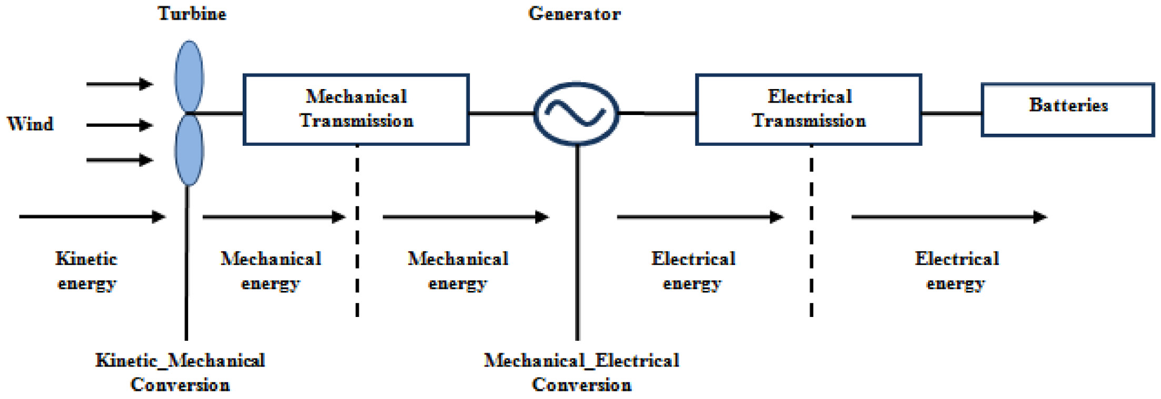
Principle of wind energy conversion.

The selected structure of the conversion chain is illustrated by the Figure 2

Figure 2.

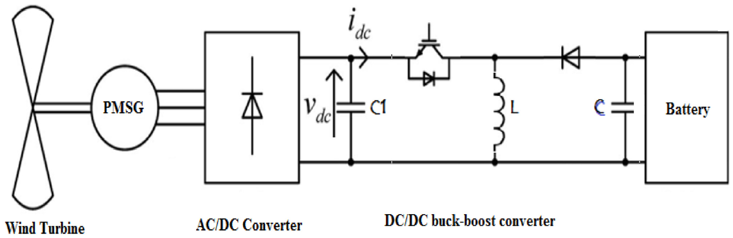
Structure of the WECS.

In order to study the WECS and to test the MPPT control algorithm on a simulation platform, it is necessary to model mathematically the wind turbine, the PMSG, and the electrical part consisting of an AC/DC converter and a DC/DC buck-boost converter.

Wind turbine modeling

There are two types of wind turbine: horizontal-axis wind turbine (HAWT) and vertical-axis wind turbine (VAWT) (Mahdavian et al., 2014). We’re inclined to use HAWT for our modeling due to their popularity driven by lower cost, lower exposure to mechanical stresses, lower starting speed and high power coefficient (Heydari and Smedley, 2015).

A wind turbine converts the energy of the air mass into motion and delivers a mechanical power characterized by the turbine rotor speed and the mechanical torque as defined in Figure 3 (Huang et al., 2015; Tan and Islam, 2004; Wei et al., 2016).

Figure 3.

Principle of the wind turbine.

The power extracted by a wind turbine is defined as:

P_{eol} = \frac{1}{2} \times C_{p} (λ, β) \times ρ \times S \times V_{w}^{3}

(1)

Where:

C_p: is the power coefficient which represents the aerodynamic efficiency of the turbine. It is a function of the pitch angle β and the specific speed λ.

λ: Specific speed, called Tip Speed Ratio (TSR)which represents the ratio between the linear velocity of the generator speed and the wind speed λ = R.Ω/ Vw.

ρ: Air density in [Kg/m³].

S: The Area swept by the blades [m²].

Ω: The angular mechanical speed of the wind turbine rotor [rad/s].

V_w: Wind speed [m/s].

R: is the blade radius [m].

Several numerical approximations have been developed in the other literatures to determine an expression of the coefficient C_p. Among these approximations, we quote the following expressions (Agarwal et al., 2010; Dalala et al., 2013; Nasiri et al., 2014; Rahim, 2014; Singh and Chandra, 2011):

First expression

C p = \frac{1}{2} . (γ - 0, 022 . β^{2} - 5, 6) . e^{- 0, 17 γ}

(2)

Where $γ = \frac{9}{4} \times \frac{Vw}{Ω}$ the peripheral velocity ratio and β represents the angle of inclination of the blade in degree.

Second expression

C_{P} = 0.73 \times (\frac{151}{λ^{'}} - 0.58 \times β - 0.002 \times β^{2.14} - 13.2) \times e^{- \frac{18.4}{λ^{'}}}

(3)

Where $\frac{1}{λ'} = \frac{1}{λ + (β . 0, 02)} - \frac{0, 003}{β^{3} + 1}$

Third expression

C_{P} = (0.44 - 0.0167 \times β) \times Sin [π \times \frac{(λ - 3)}{15 - (0.3 \times β)}] - (0.00184 \times (λ - 3) \times β)

(4)

Fourth expression

C_{P} = 0.5176 \times (\frac{116}{λ'} - 0.4 \times β - 5) \times e^{- \frac{21}{λ'}} + 0.0068 \times λ

(5)

Where $\frac{1}{λ'} = \frac{1}{λ + (0, 08 . β)} - \frac{0, 035}{(3 . β) + 1}$

This last expression is part of the SIMULINK library, thus it will be the one used to validate our wind system model. The curve of the latter formula is given by Figure 4. The C_p family of curve is obtained with different value of λ and with changing β value. This dependence is clearly visually. However, the power coefficient is maximal when β = 0. So, to have best results, next simulations are carried with β = 0.

Figure 4.

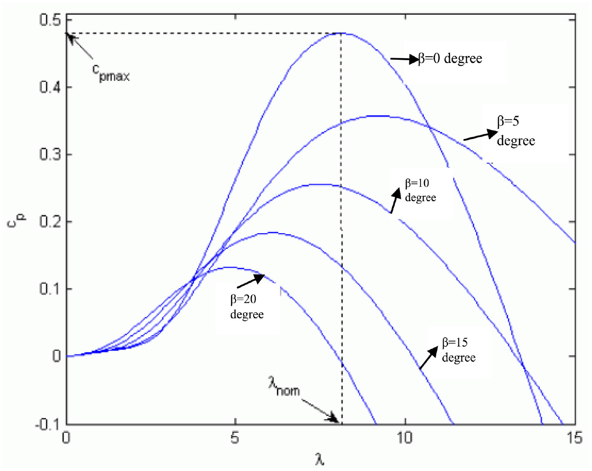
Aerodynamic power coefficient variation C_p against TSRλ and the pitch angle β.

The expression of the torque corresponding to the power previously mentioned is given by:

C_{eol} = \frac{P_{eol}}{Ω} = \frac{1}{2} \times \frac{Cp (λ) \times ρ \times S \times V_{w}^{3}}{Ω}

(6)

The mechanical torque seen by the synchronous machine is different from the wind couple because it is necessary to account for inertia of the wind turbine and of the viscous friction peculiar to the wind turbine. This can be translated into mathematical terms by the following equations:

C_{eol} = J \times \frac{d Ω}{dt} + f \times Ω + C_{mec}

(7)

Ω = \frac{1}{f + p \times J} \times (C_{eol} - C_{mec})

(8)

Wherein J and f are respectively the inertia and the friction of the wind turbine. P is the Laplacian operator. From these two equations we can represent the dynamic model of the wind turbine with Figure 5:

Figure 5.

dynamic model of the wind turbine.

PMSG model

The PMSG modeling consists in constructing a mathematical model of the machine, reflecting the electromagnetic and mechanical phenomena that govern its operation. This makes it possible to study with pertinence, the behavior of the different variables in dynamic and static mode and to exploit this model in simulations (Balasundar et al., 2015; Nasiri et al., 2014).

By neglecting the saturation of the magnetic circuit, the hysterical losses and assuming that the tensions are sinusoidal, the system of voltage equations of the synchronous machine is given by the following equations:

va = - Ra \times ia + \frac{d ψ a}{dt}

(9)

vb = - Rb \times ib + \frac{d ψ b}{dt}

(10)

vc = - Rc . \times ic + \frac{d ψ c}{dt}

(11)

Where Ra = Rb = Rc = Rs the stator resistances and ψa, ψb, ψc respectively the totals fluxes circulating in the stator windings of the phases a, b, and c. For simplicity, we write this system in matrix form with the following equation:

[v_{abc}] = - Rs \times [i_{abc}] + [\frac{d ψ_{abc}}{dt}]

(12)

In order to simplify the calculations even more, it is preferable to use a biphase reference. This is done using the Park-Clark transform (Figure 6). The PMSG model can be written, in the d-q synchronously rotating reference frame (Gragger et al., 2010; Mirecki, 2005).

Figure 6.

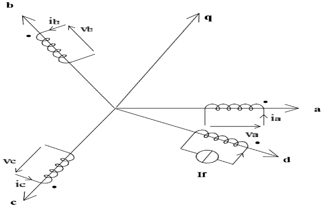
Park-Clarkereference.

The Park-Clark matrix is given by:

P (θ) = \frac{2}{3} \times [\begin{matrix} \cos (θ) \cos (θ + \frac{2 \times π}{3}) \cos (θ + \frac{4 \times π}{3}) \\ \sin (θ) \sin (θ + \frac{2 \times π}{3}) \sin (θ + \frac{4 \times π}{3}) \end{matrix}]

(13)

Where $[\begin{matrix} Xd \\ Xq \end{matrix}] = P (θ) \times [\begin{matrix} Xa \\ Xb \\ Xc \end{matrix}]$

By applying the Park transformation according to the synchronous two-phase reference (d, q) linked to the field Stator, to the magnitudes of voltages, currents and flux, the system of voltage equation will be reduced to:

v_{ds} = - R_{s} \times i_{ds} + ω_{r} \times L_{q} \times i_{qs} - L_{d} \times p \times i_{ds}

(14)

v_{qs} = - R_{s} \times i_{qs} - ω_{r} \times L_{d} \times i_{ds} + ω_{r} \times ψ_{r} - L_{qs} \times i_{qs}

(15)

These equations can be represented as shown in Figure 7 by the following equivalent electrical schemes:

Figure 7.

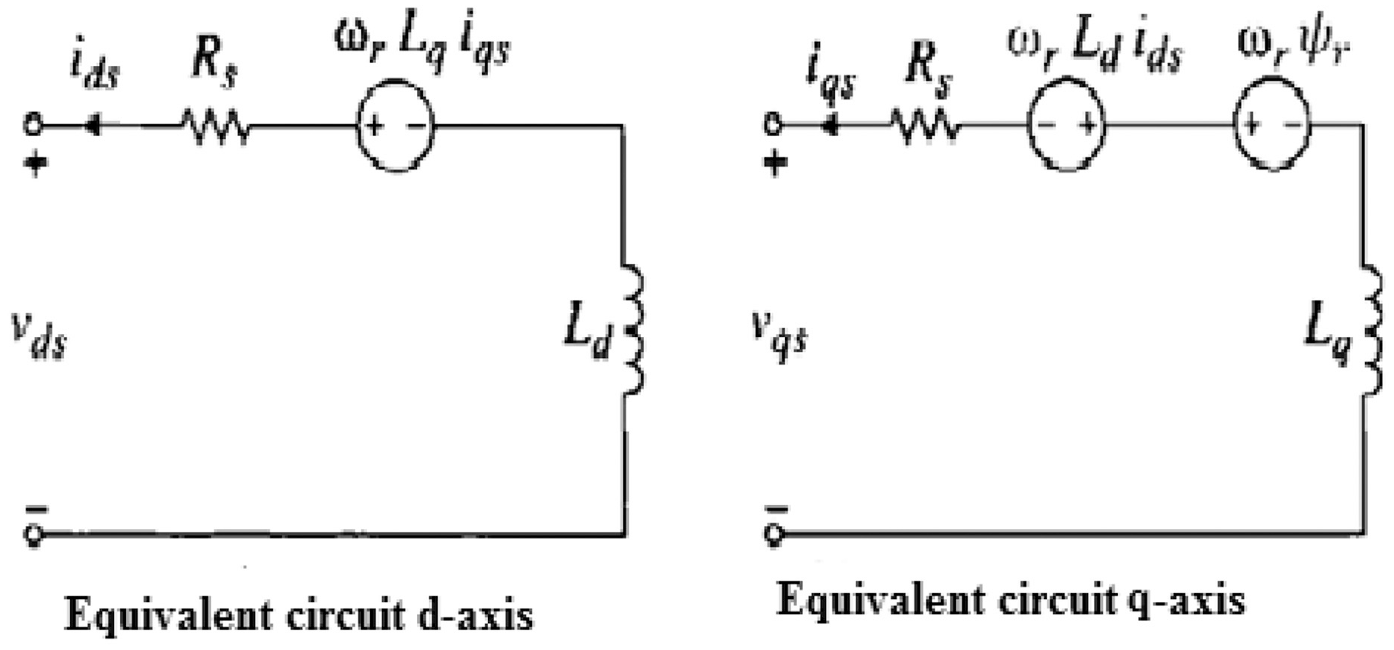
Electric circuit equivalent to the PMSG model.

The expression of the electromagnetic torque is given by:

T_{e} = \frac{3 \times N_{p}}{2} \times [i_{qs} \times ψ_{r} - (L_{\partial} - L_{q}) \times i_{ds} \times i_{qs}]

(16)

Wherein N_p is the number of pole pair.

The expression of the rotor pulsation is as follow:

ω r = \frac{N_{p}}{J \times p} \times (T_{e} - T_{m})

(17)

Three-phase diode rectifier bridge

Given that the PMSG produces a variable frequency and amplitude voltage, additional power electronics are required to satisfy the charge requirements. The method often used is to straighten the output voltage. In this study, a three-phase diode bridge is used to rectify the voltage generated by the PMSG (Neji et al., 2006).

The circuit constituted by a diode bridge (PD3) of Figure 8 is considered, the diodes are assumed to be perfect (perfect switches) and the current at the output of the rectifier assembly is continuous (Strongly inductive load).

When v1 > v2 > v3, D1 and D’3 lead: ud = v1 − v3;

When v1 > v3 > v2, D1 and D’2 lead: ud = v1 − v2;

When v2 > v1 > v3, D2 and D’3 lead: ud = v2 − v3;

When v2 > v3 > v1, D2 and D’1 lead: ud = v2 − v1;

When v3 > v1 > v2, D3 and D’2 lead: ud = v3 −v1;

When v3 > v2 > v1, D3 and D’1 lead: ud = v3 −v2

Figure 8.

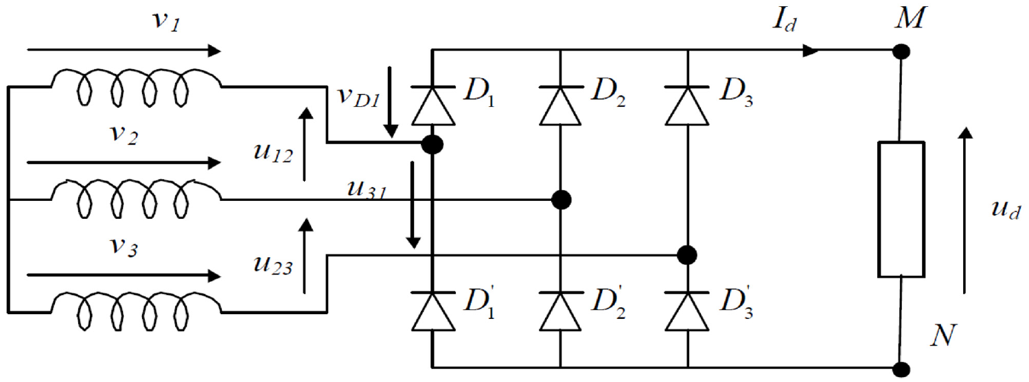
Three-phase diode Rectifier Bridge.

Each diode thus conducts for one-third of a period while the rectified voltage consists of six portions of ideal sinusoid per period T. In Figure 9, the graph of the rectified voltage and the voltage at the terminals of the diode D1 are presented.

Figure 9.

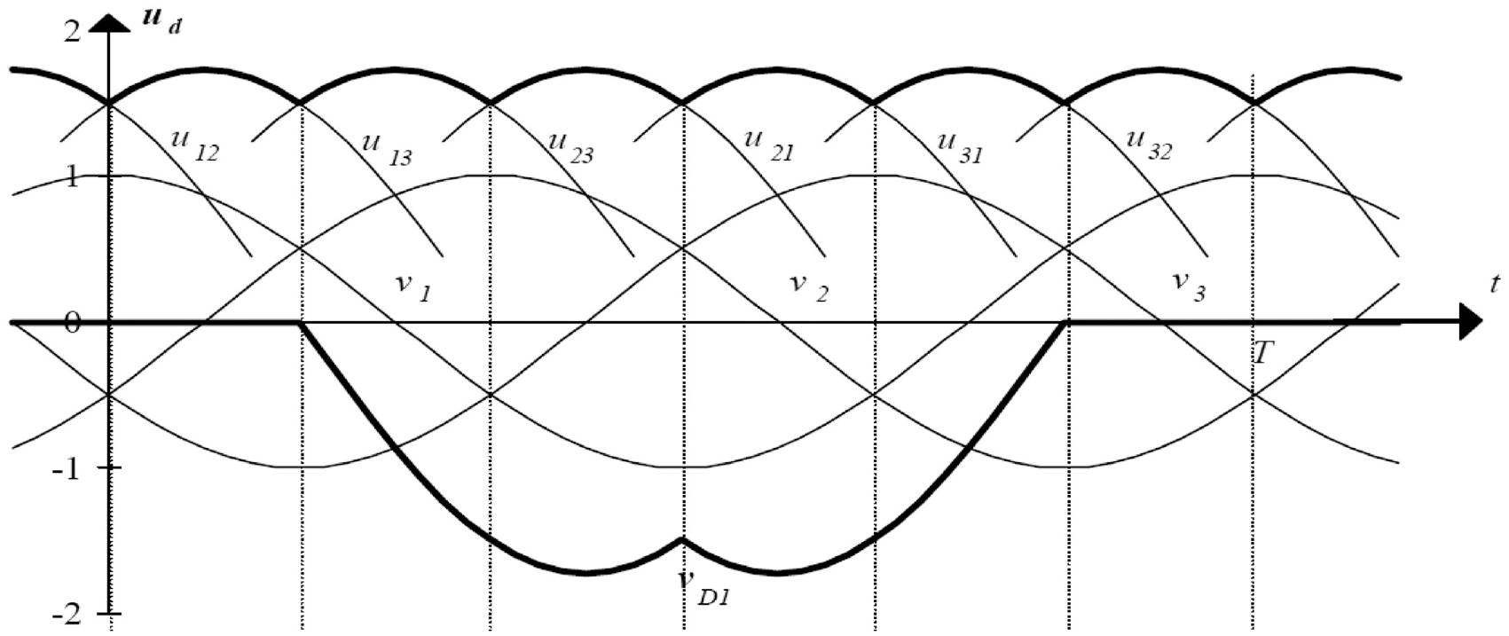
The rectified voltage.

We have assumed that the source and the rectifier are perfect, whereas the rectified voltage U_d is periodic per period T/6. Between 0 and T/6, this tension is expressed: U_d = Us.√2.cos (w t) with U_s being the effective value of the input voltages. Given that the elements are not perfect (the fall due to resistors and diodes, the accumulation, the non-sinusoidal of input voltage ...) leads to a decrease of the mean value Ud of the rectified voltage. This fall can be neglected.

In this case, we have:

U_{d} = \frac{1}{\frac{T}{6}} \times \int_{- \frac{T}{12}}^{\frac{T}{12}} u_{d} \times dt = \frac{3 \times \sqrt 6}{π} \times U_{PMSG}

(18)

I_{d} = \frac{π}{\sqrt 6} \times I_{PMSG}

(19)

Wherein U_d and I_d are the mean values of the voltage and the output current of the rectifier, U_PMSG and I_PMSG are the values of the fundamental voltage and current alternative side

The DC/DC converter choice and modeling

The constraints of cost and simplicity favor the choice to optimize the DC side power by combining a DC/DC converter with rectifier diodes. In order to better choose the type of DC/DC converter to use, it is necessary to take into account certain risks:

- The wind speed range on which the wind turbine is to operate.

- The maximum and minimum stops of the duty cycle.

- The battery voltage.

- The two factors Fd, Ae.Sb represent respectively the Over-dimensioning of a switch as “silicon” and the criterion of dimensioning of the smoothing inductance of the converter (where Ae is the section Equivalent of the magnetic core and Sb the winding section).

For a buck DC/DC converter its two factors are penalizing against structures based on a boost DC/DC converter or buck-boost DC/DC converter. Thus, the structure chosen is that of the buck-boost DC/DC converter shown in Figure 10, since it allows operation on a wider range of wind speed (Pertuza, 1996; Tounsi et al., 2006).

Figure 10.

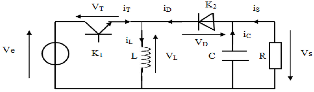
The inverter buck-boost DC/DC converter configuration.

The transfer functions of the inverter buck-boost DC/DC converter in continuous conduction mode are given by the following equations:

\frac{\tilde{v} s}{\tilde{α}} = (\frac{Vs}{α \times (1 - α)}) \times (\frac{(1 - (\frac{α \times L}{R \times {(1 - α)}^{2}}))}{1 + (\frac{L \times p}{R \times {(1 - α)}^{2}}) + (\frac{L \times p^{2}}{C \times {(1 - α)}^{2}})})

(20)

\frac{\tilde{v} s}{\tilde{v} e} = \frac{α}{1 - α} \times (\frac{1}{1 + (\frac{L \times p}{R \times {(1 - α)}^{2}}) + (\frac{L \times p^{2}}{C \times {(1 - α)}^{2}})})

(21)

\frac{\tilde{v s}}{\tilde{i L}} = R \times \frac{(1 - α)}{(1 + α)} \times \frac{1 - (\frac{(α \times L \times p)}{R \times {(1 - α)}^{2}})}{1 + (\frac{R \times C \times p}{1 + α})}

(22)

In this paper, we are interested in regulating the DC/DC converter output voltage, so as to recharge the battery, by acting on the ratio cyclic α. Thus, we are concerned with the first equation among the three quoted above. This will allow us to better dimension the elements of the converter, in particular inductance.

MPPT commands for WECS

In the previous section we have presented the mathematical model of the different elements constituting our WECS. In this section, we define the power maximization algorithms used for wind turbines.

The MPPT control must comply with the constraints of simplicity and cost without impairing efficiency. We can distinguish between two main categories of MPPT strategies: strategies requiring prior knowledge of the characteristic C_p (λ) of the wind turbine (indirect methods), and strategies that do not require knowledge of this characteristic curve (direct methods) (Blaabjerg et al., ; Haque et al., 2010).

A disadvantage of the indirect methods is that the power curve of a wind turbine is not available with high precision and will change after the rotor oldness. Another disadvantage is that it requires the wind speed measurement. The anemometers price is a barrier for the indirect methods application in isolated sites. Thus, our choice falls on the second one (Neji et al., 2006).

The MPPT control strategies without knowledge of the characteristic curve are based on heuristic algorithms which make it possible to know and track the maximum power constantly without prior knowledge of any component of the wind energy conversion chain, namely the characteristic C_p = f(λ) of the wind turbine, the PMSG (Balasundar et al., 2015; Dalala et al., 2013; Gragger et al., 2010; Marouani and Tounsi, 2014; Mirecki, 2005; Nasiri et al., 2014; Nasri and Tounsi, 2015; Neji et al., 2006, 2006; Pertuza, 1996; Singh and Chandra, 2011; Suilah et al., 2015; Tounsi, 2015; Tounsi et al., 2006; Tounsi, 2015).

The basic P&O strategy

The P&O algorithm (Perturb and Observe) is one of the simplest algorithms. It consists of the introduction of a small perturbation of the cyclic ratio. Its effect is subsequently noticed at the level of the output power of the PMSG. If an increase in electrical power is recorded by the increase of the duty cycle, then the duty cycle is going to be increased again with the same step as the preceding one. If, on the other hand, a decrease of the power is recorded following the increase of the duty cycle, the following set point of cyclical ratio is then reversed (Agarwal et al., 2010; Balasundar et al., 2015; Dalala et al., 2013; Gragger et al., 2010; Mirecki, 2005; Nasiri et al., 2014; Nasri and Tounsi, 2015; Neji et al., 2006, 2006; Pertuza, 1996; Rahim, 2014; Singh and Chandra, 2011; Suilah et al., 2015; Tan and Islam, 2004; Tounsi et al., 2006).

Figure 11 shows the algorithm described.

Figure 11.

Basic P&O algorithm.

Where k is the current iteration and k-1 is the previous iteration.

Basic P&O control, however, has some disadvantages related to:

Oscillation of output power is permanent even during fixed wind speeds.

The Slowness of finding the point of extraction of the maximum power by strategies with knowledge of the characteristic of the wind turbine because the variation pitch of the duty cycle is fixed.

This maximum power’s research strategy does not allow the detection of small transient wind variations. Thing that may generate unwanted and erroneous power variations.

To overcome all the basic P&O drawbacks, we propose a technique that combines the advantages of advanced P&O and the speed of ORB control (Optimum Relationship-Based control) without the need to know beforehand the characteristics of the system.

Advanced P&O combined with ORB

The maximum output power of the AC/DC converter is given by:

P_{dc - \max} = η_{dc} \times K_{opt} \times Ω_{opt}^{3} = K_{opt'} \times Ω_{opt}^{3}

(23)

Wherein η_dc is the yield of the PMSG and the DC/DC converter.

We can consider that the voltage V_dc is proportional to the generator angular speed Ω (neglecting the losses in the PMSG) via the relation:

Ω = \frac{V_{dc}}{\frac{3 \times \sqrt{6}}{π}} \times ψ_{eff} \times k

(24)

We can therefore write:

P_{dc - \max} = K_{opt}^{"} \times V_{dc - opt}^{3}

(25)

We also have the relationship:

P_{dc - \max} = V_{dc - opt} \times I_{dc - opt}

(26)

By replacing the expression of P_dc−max in the previous relation, we find that an operating at maximum power amounts to respecting a proportional relationship between Current Optimal output of the AC/DC converter I_dc−opt, and the square of the optimal voltage V²_dc−opt, which amounts to writing:

I_{dc - opt} = K_{opt}^{"} \times V_{dc - opt}^{2}

(27)

The MPPT Strategy that we have proposed is based on two modes of control, namely a mode consists in finding the relation K opt′′ via the advanced P&O algorithm, and one mode based on the optimal relationship control (ORB control) which consists in using the relationship K opt′′′in the rest of the MPPT strategy using an ORB control.

Figure 12 gives the curve I_dc = f (V_dc²) for different wind speeds. The Line on the curve on the left represents the line of the pairs (I_dc−opt, V_dc−opt²) for which the withdrawn power of the wind turbine is maximum.

Figure 12.

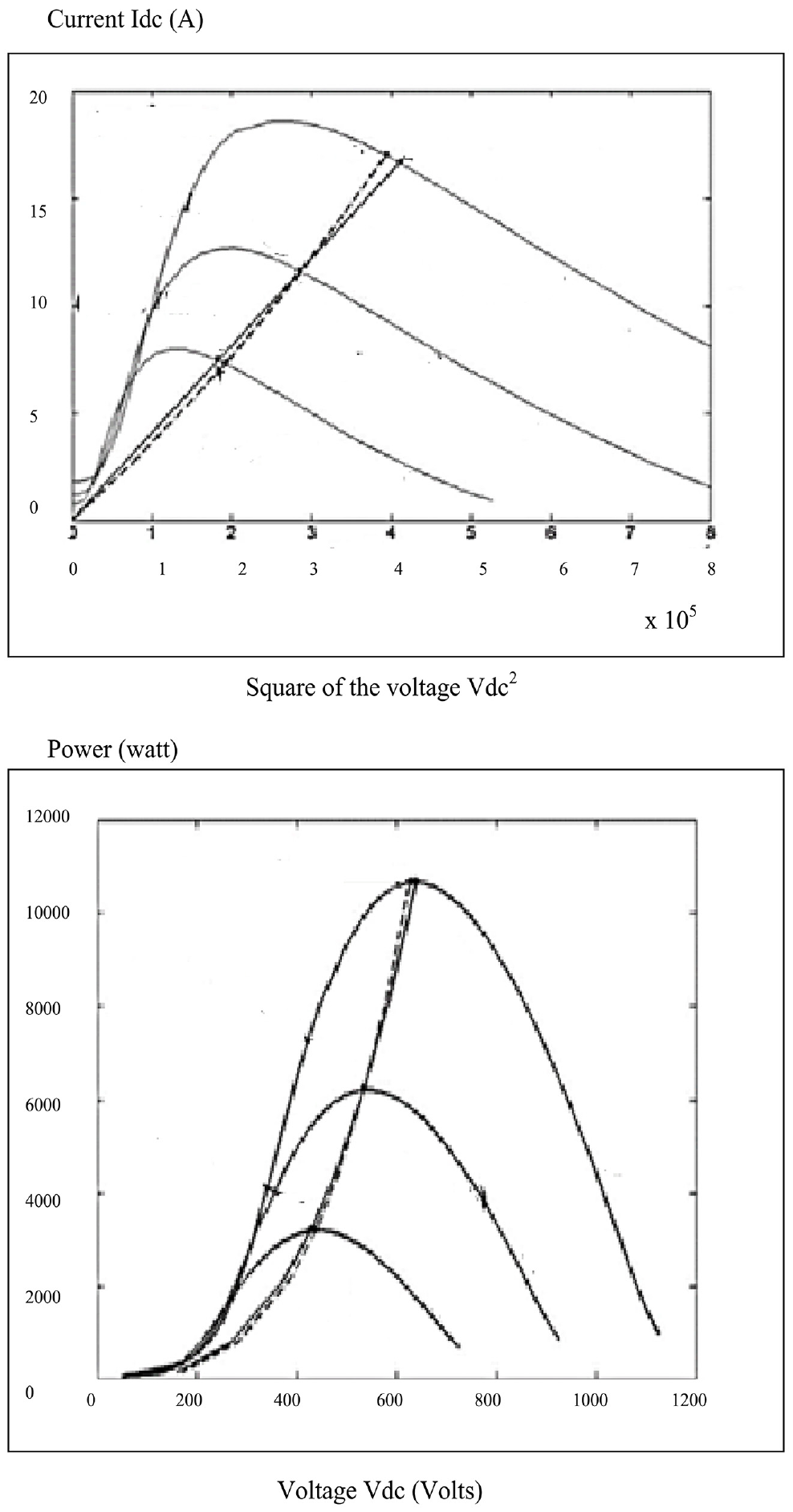
Characteristic curve of the current as a function of the voltage and power as a function of the voltage.

From this curve, it is also possible to write:

I_{dc - opt} = α \times \tan (θ_{opt}) \times V_{dc - opt}^{2}

(28)

Wherein α = I nominal/V²nominal

The aim of our algorithm is to find therefore this ratio K_opt (respectively the angle θ_opt) making it possible to track subsequently the maximum power.

Figure 13 describes the adopted algorithm that will be translated into script on the Matlab-function block.

Figure 13.

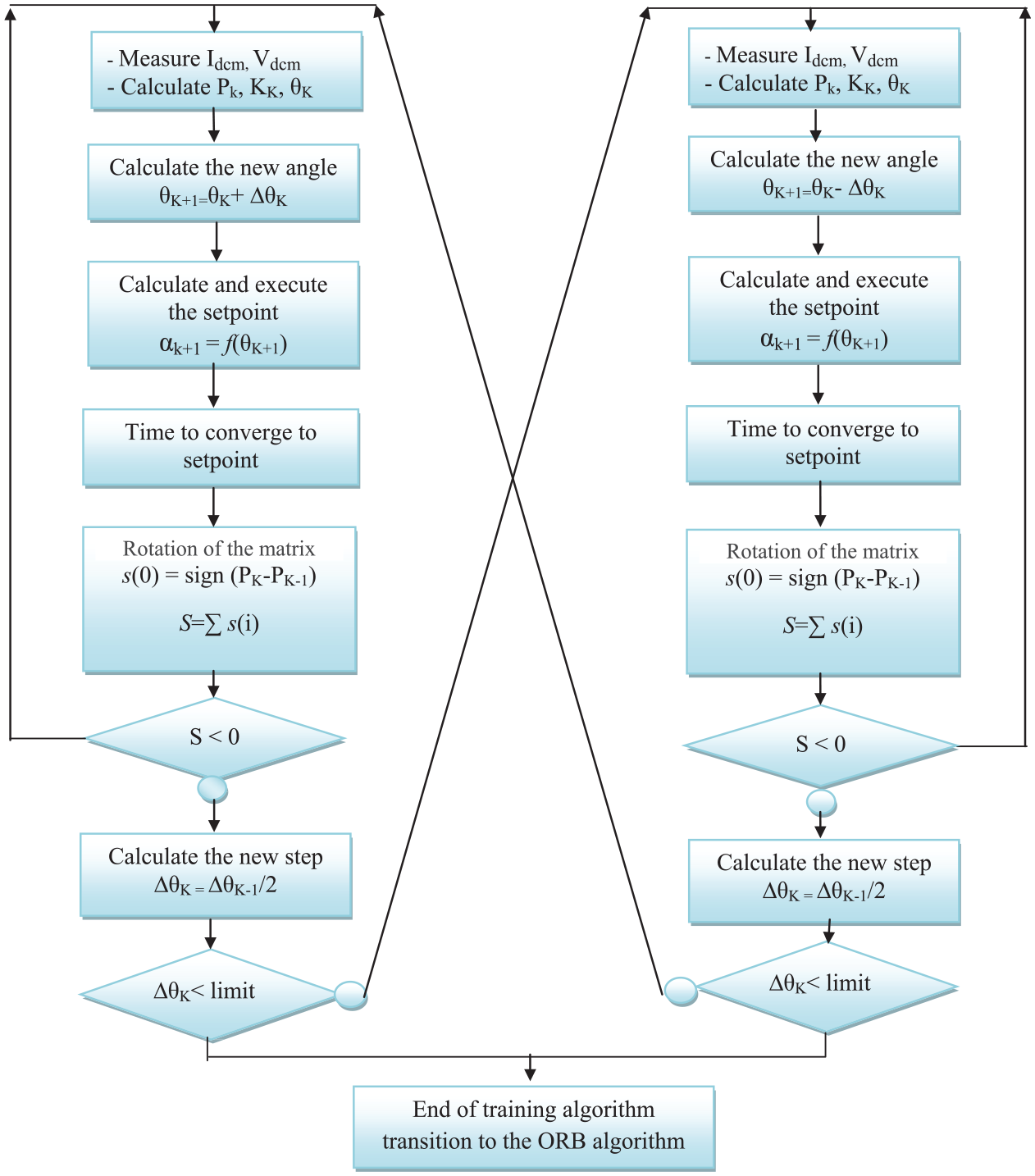
Organization chart of the P&O advanced algorithm.

The training algorithm cited above and the control by the ORB algorithm are part of the same set since the latter depends on the optimal relationship found by the training algorithm. They were separated in order to be able to see separately the functioning of each one. The Optimal Relation Based Control (ORB) algorithm is based on the optimal angle θ (respectively the K_optimal ratio) which connects the optimal voltage to the optimum current. We use this ratio in order to assign successive instructions of the cyclic ratio α which will converge to optimal.

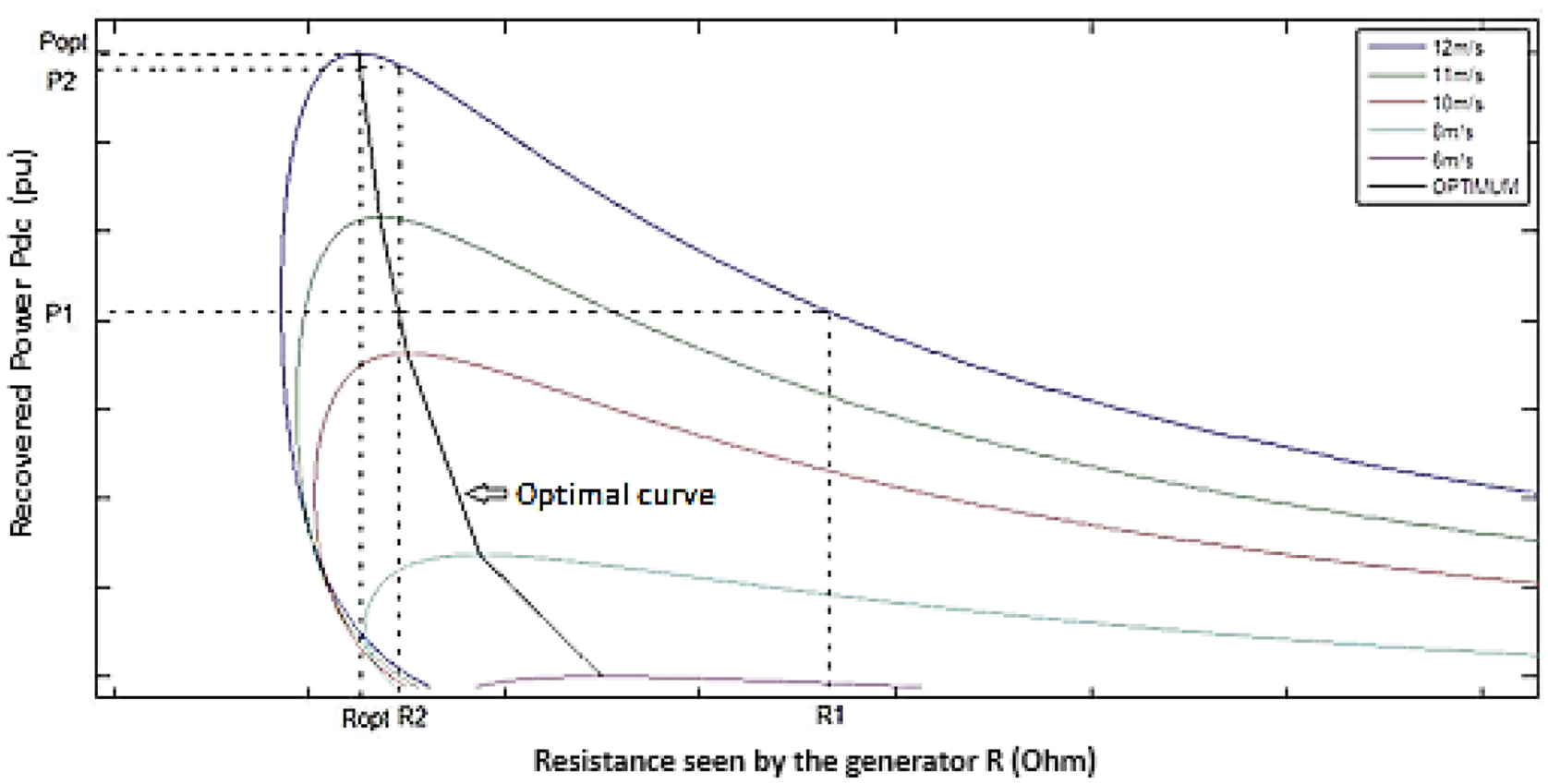
With this last setpoint of the duty cycle, the resistance seen by the generator is that which maximizes the power

The convergence of the search for the maximum power point is carried out according to the following steps:

By measuring the current I_dc0, the K_opt ratio allows us to determine a new reference voltage V_{dc_ref1} by the relation.

V_{dc - ref 1} = \sqrt{\frac{I_{dc 0}}{K_{opt}}}

(29)

The resistance which is to be seen by the generator is determined at this reference voltage.

R_{dc - ref 1} = \frac{V_{dc - ref 1}}{I_{dc 0}}

(30)

By measuring the load resistance R_ch at the output of the DC/DC Converter. The cyclic ratio allowing to modify the resistance seen by the generator is then calculated according to the following equation:

α_{ref 1} = \frac{1}{1 + \sqrt{\frac{R_{dc - ref 1}}{R_{ch}}}}

(31)

After a calculation period, the system state equivalent to (R1, P1) is reached and the new reference resistance R_{dc_ref2}is calculated.

After several iterations, the optimal point (R_opt, P_opt) is reached.

Description of simulations results

In this section, we will present the model of our WECS in the MATLAB_SIMULINK environment. The objective is to test different Maximum Power Point Tracking (MPPT) algorithms, and validate the optimized algorithm cited in the previous section, based jointly on the advanced P & O (Perturb and Observe) and the ORB (Optimum Relationship Based Control).

Simulink model presentation

The proposed system is a wind turbine driving a permanent magnet synchronous machine to charge a battery. This type of application is often located in an isolated site not connected to the electricity grid. However, the validation of an algorithm for extracting the maximum power remains a matter of concern for all players in the wind energy sector, whether small power or high power.

The mode of the proposed WECS is given by the Figure 14

Figure 14.

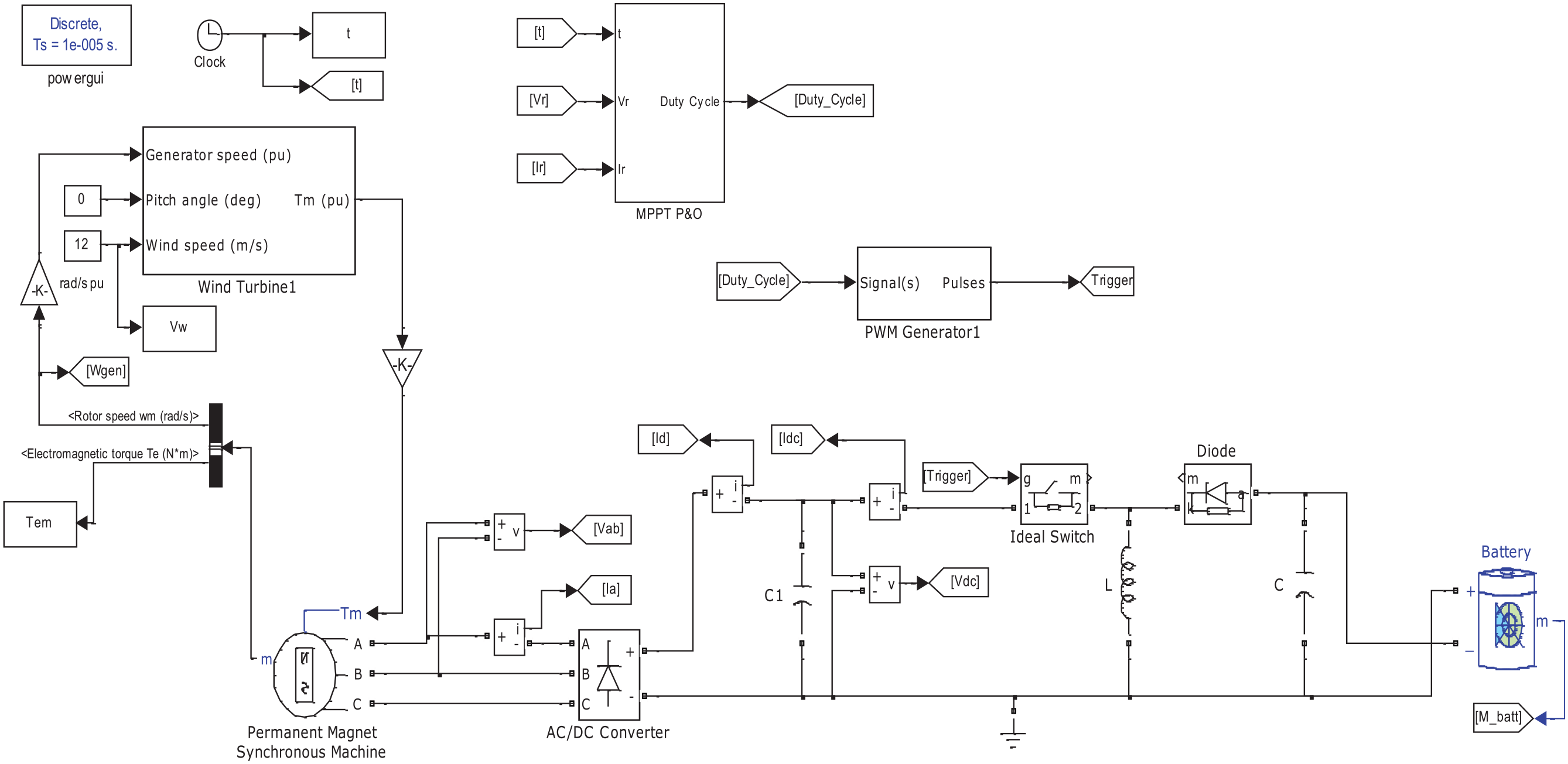
Model of the WECS in SIMULINK.

The wind turbine model in the Simulink SimPower library is identical to the modeling given in section2. In this simulation we propose to study the Behavior of a wind turbine that produces 2.4 KW for a nominal wind speed of 12 m/s. All the parameters of the wind turbine are given in the Figure 15:

Figure 15.

Wind turbine parameters.

Unlike the mathematical model given in section 3, the Simulink model of the wind turbine does not include the mechanical equation of the wind turbine. This equation must be added either in a separate block by adding the inertia of the turbine to that of the generator. For reasons of simplicity we opt for the second choice, as recommended by the documentation on Matlab (Gragger et al., 2010; Marouani and Tounsi, 2014; Mirecki, 2005; Nasri and Tounsi, 2015; Neji et al., 2006, 2006; Pertuza, 1996; Suilah et al., 2015; Tounsi, 2015; Tounsi et al., 2006; Tounsi, 2015).

Figure 16 shows the wind turbine mechanical equation model in Simulink:

Figure 16.

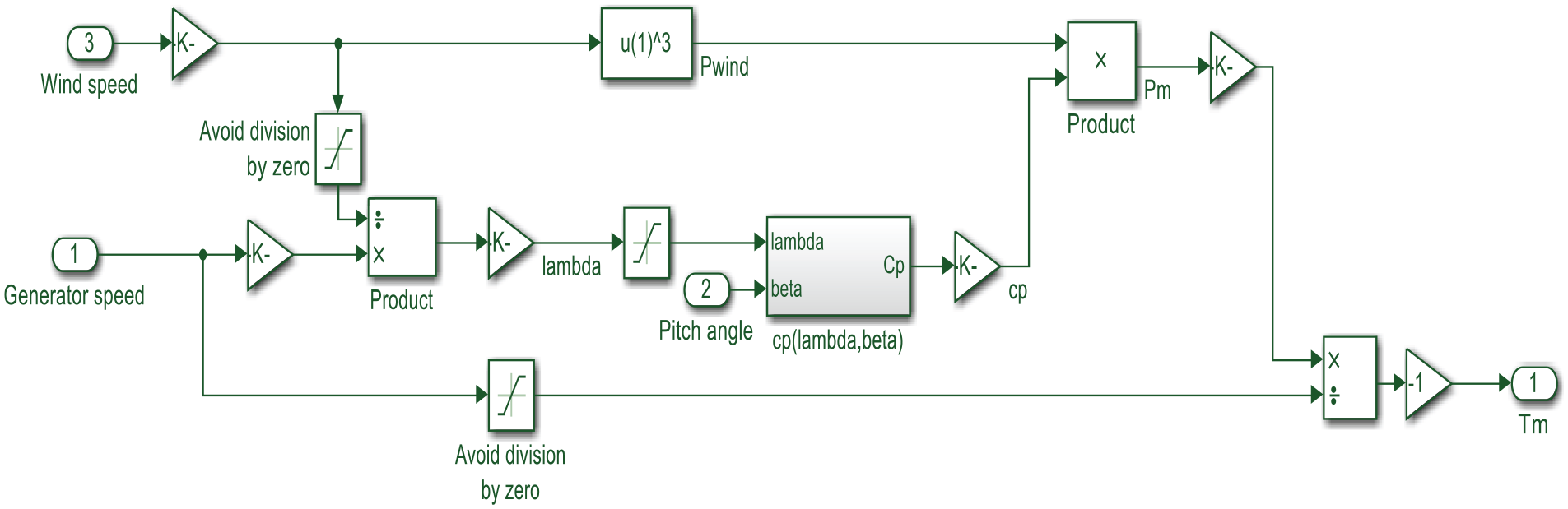
The wind turbine mechanical equation model.

The equation of C_p = f (λ) of this model is given by the Figure 17 below. The wind turbine reaches a maximum value of C_p of 0.8 for an optimal specific speed λopt = 8.

Figure 17.

C_p function model in Simulink.

The model used for the generator is also present in the SimPower library. We will use a PMSG with smooth poles whose specifications techniques are given in Table 1:

Table 1.

Simulation parameters.

Parameters	Value
Nominal power	3 KW
Nominal voltage	220 V
Stator resistance	0.49 Ohm
Stator inductance	5.35 mH
Torque constant	2.4 Nm/A
Number of poles	4
Yield	87.3%

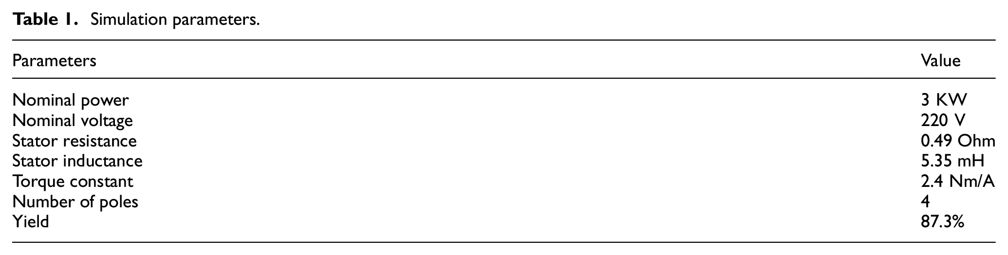
The design and control parameters are extracted from analytical design model of the power chain.

The trigger signal of the DC/DC converter IGBT switch will be governed by a PWM generator. The Block diagram on Simulink of the PWM generator is given Figure 18:

Figure 18.

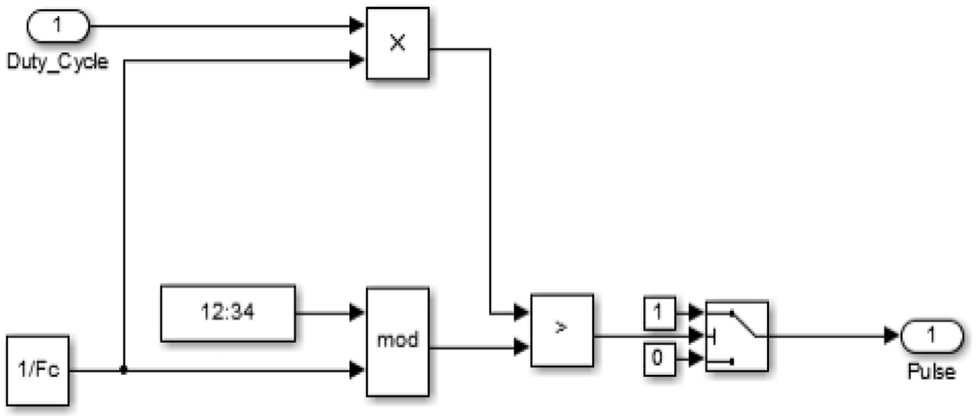
PWM Generator.

The calculation of the duty cycle value will be done via an algorithm as explained in section 3. The way to develop an algorithm on Matlab is to use the tool “Matlab Function.” This block allows to write lines of commands which all execute, line by line during each simulation cycle during SIMULINK simulation.

Simulations results

The power and torque curves as a function of the generator rotational speed according to wind speeds are given in the Figures 19 and 20.

Figure 19.

The power curves as a function of the generator rotational speed.

Figure 20.

The torque curves as a function of the generator rotational speed.

We drive the wind turbine by a wind speed equal to 12 m/s (Figure 21). We expect the rotational speed of the rotor and the power to stabilize. And then we run the P & O algorithm

Figure 21.

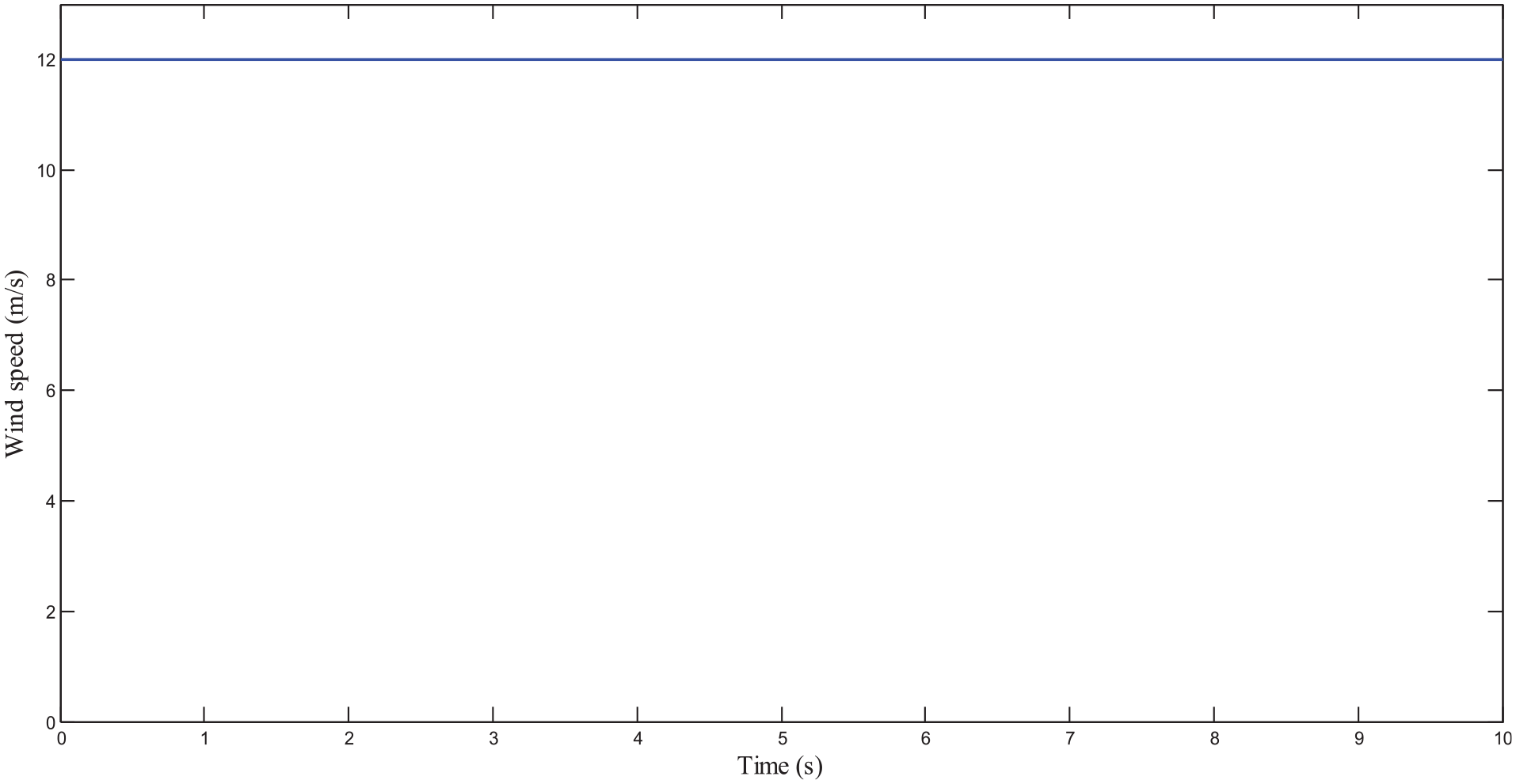
Wind speed.

After running the simulation, we find the evolution of the following quantities: power coefficient C_p, duty cycle α, recovered power Pdc, and generator rotational speed Ω_gen as shown respectively in Figures 22 to 25. The power curve is displayed in reduced value compared to the nominal value of 2400W. With this algorithm we have varied the duty cyclic to change the impedance seen by the generator, resulting in a respective variation of the rotor speed, power coefficient, thus we optimized the captured power of the wind turbine. This power, which only reached 70% in free operation, can now reach 95% of the nominal power.

Figure 22.

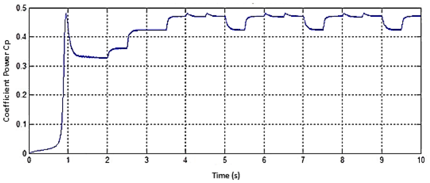
Power coefficient C_p evolution as a function of time.

Figure 23.

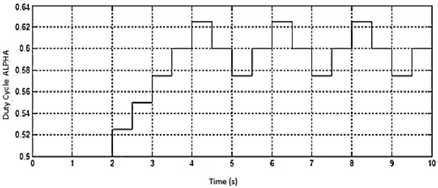
Duty cycle evolution as a function of time.

Figure 24.

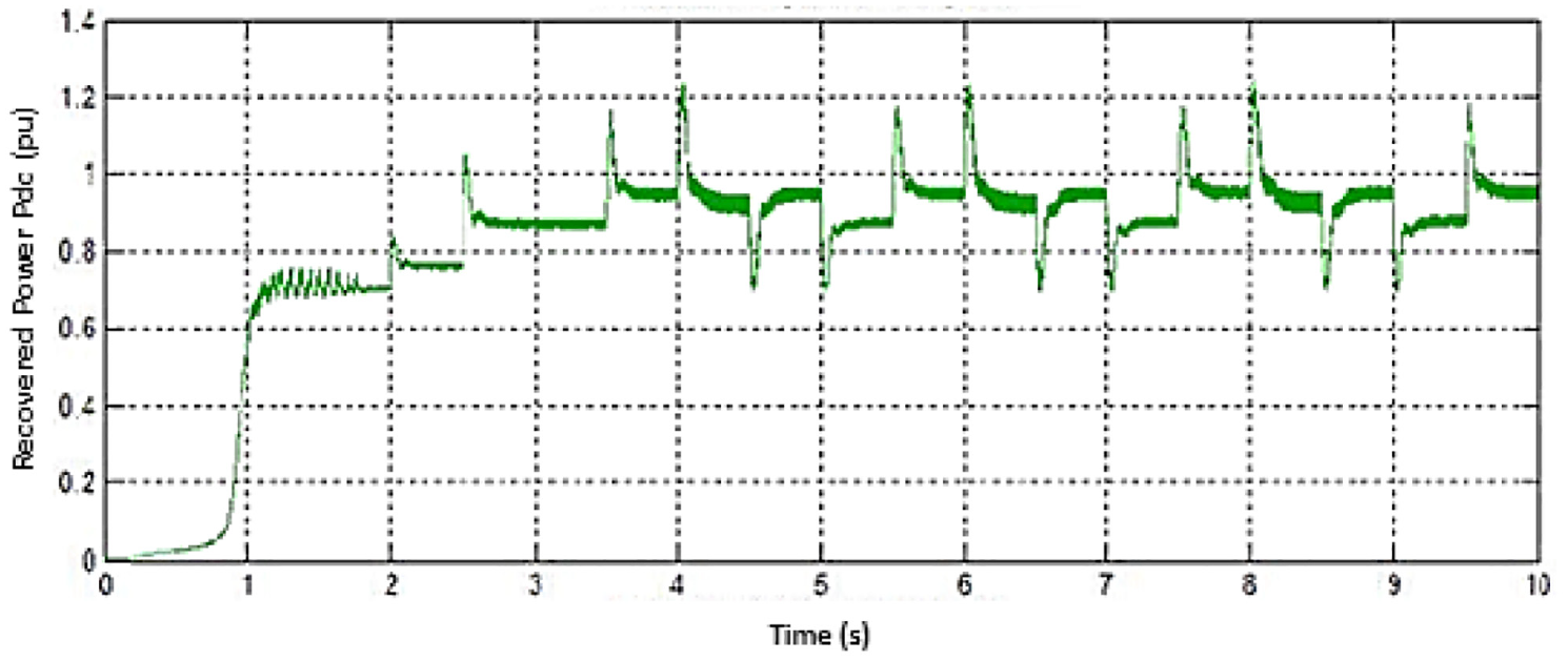
Recovered power evolution as a function of time.

Figure 25.

Generator rotational speed evolution as a function of time.

Since the P&O algorithm is based on permanent perturbations, the power is never fixed even in the presence of a stable wind speed. In our case the power oscillates between 87% and 95%. Another disadvantage of the P&O algorithm is that in the presence of wind variations, the algorithm may take decisions on wrong variations (such as a drop in wind speed while optimum C_p is not yet reached). The performance of the power maximization system will therefore be reduced in the presence of changes in wind speed.

In order to remedy these disadvantages the algorithm for which we opt is divided into two parts as explained in section 4. The first part of the algorithm consists in exploring the system and finding the optimal relation between the current I_dc and the square of the voltage V_dc. The second part of this algorithm consists in exploiting this relation in order to use an algorithm which converges rapidly to find the maximum operating point of the wind turbine.

We drive the wind turbine with a wind speed of 12 m/s and we wait for the power to stabilize. This corresponds to operation on an arbitrary angle line lying around the starting line of operation as shown in Figure 26. We vary this angle according to the “advanced P&O” algorithm, until an optimal angle is reached. The angle θ_opt corresponds to the optimal operating line shown in Figure 26.

Figure 26.

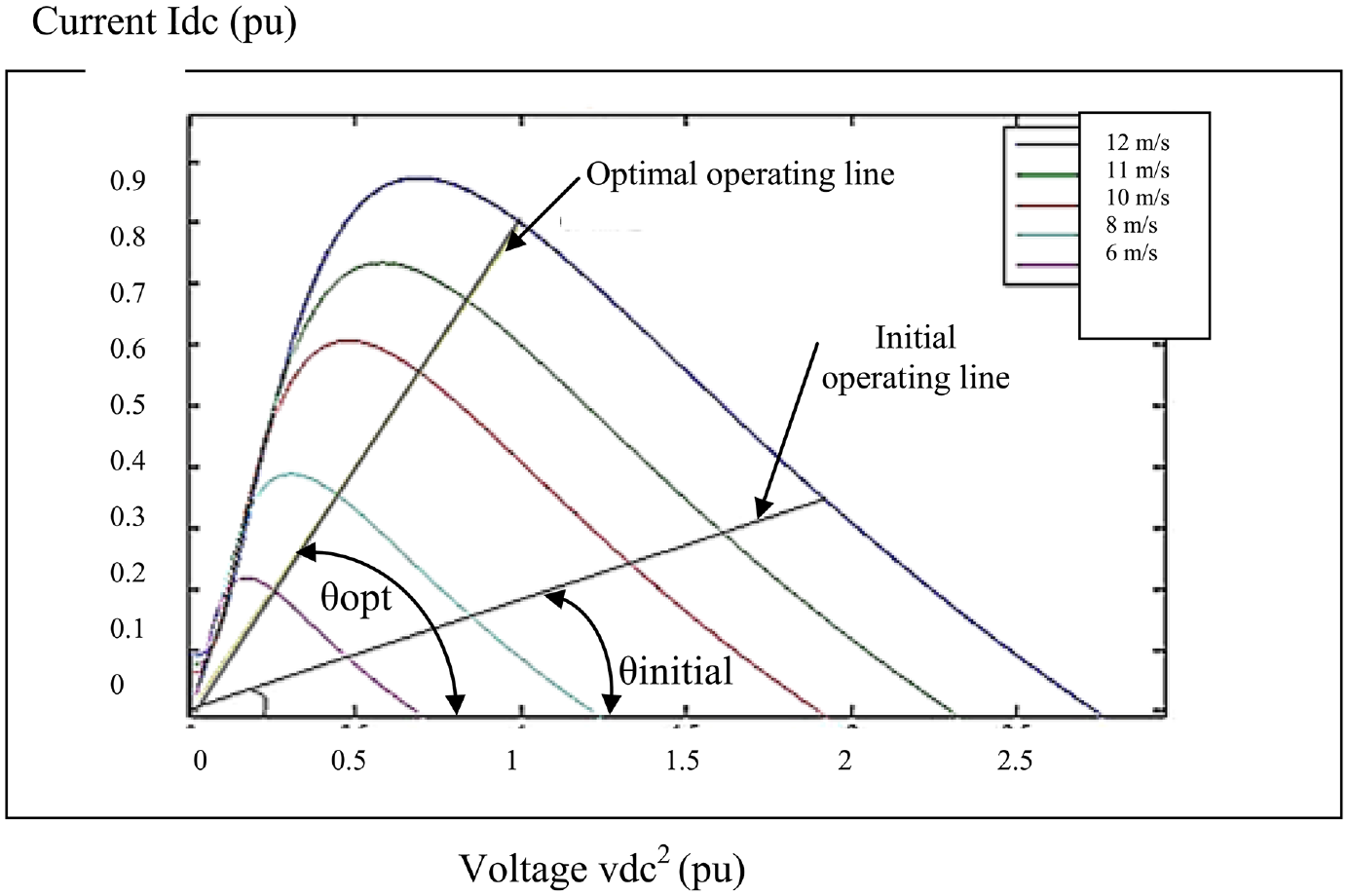
Optimal voltage and current curve.

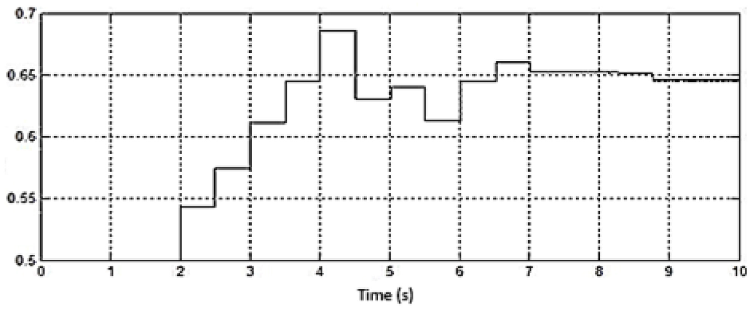
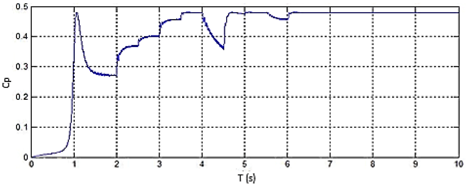
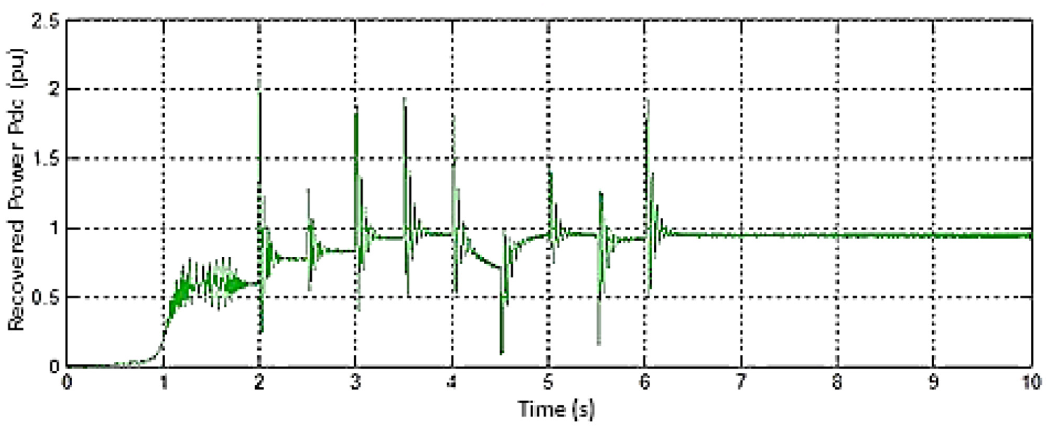
After execution of the simulation we find the following values: the angle θ, the duty cycle α, the power coefficient C_p, and the captured electric power P_dc as shown respectively in Figures 27 to 30.

Figure 27.

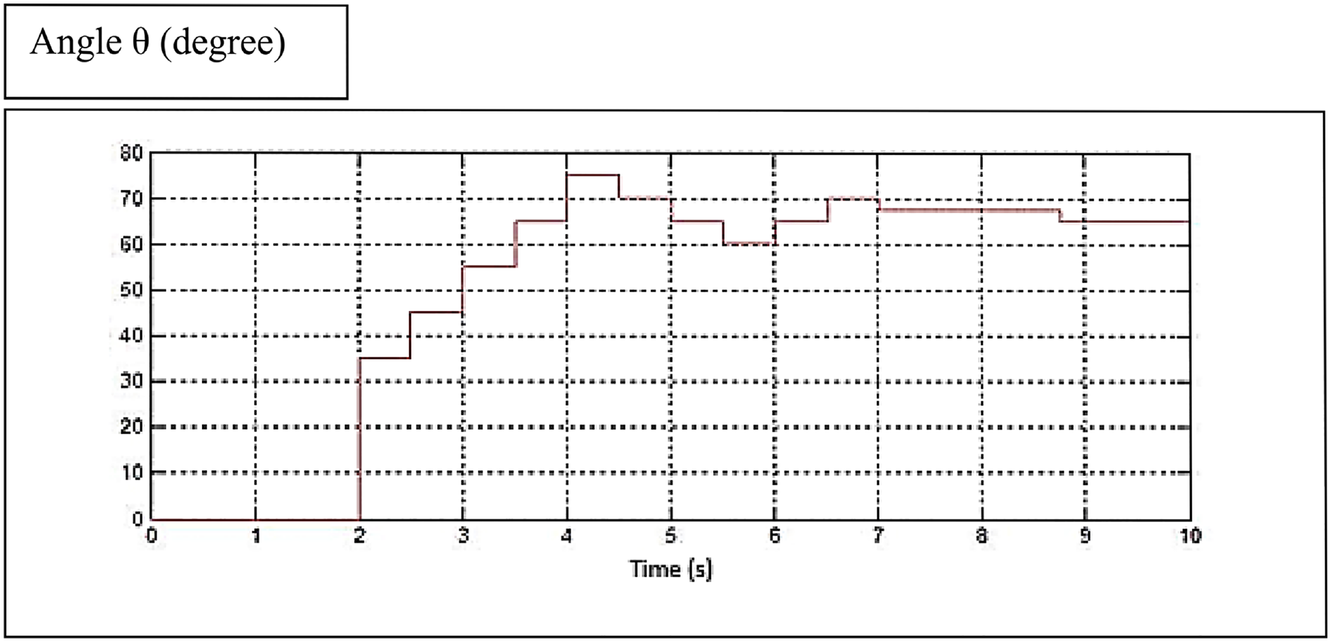
Angle’s Theta (θ) variation as a function of time.

Figure 28.

Duty cycle (α) variation as a function of time.

Figure 29.

Power coefficient C_p evolution as a function of time.

Figure 30.

Captured electric power evolution as a function of time.

After the power stabilization, the angle θ measured is 35°. Once the training algorithm is executed, the Theta angle changes, and once the optimal angle is exceeded, it begins to oscillate around this angle. The amplitude of this oscillation decreases progressively until it converges to Theta Optimal θopt = 65°, which corresponds to C_p^max = 0, 48.Thus the maximum power at the end of the dressing mode has been reached.

In the following paragraph we will test the performance of the system in tracking the maximum power in the presence of fluctuations in wind speed, using the regulation by angle θ_opt, which we have just found.

We start this simulation by driving the wind turbine with a wind speed of 12 m/s. We wait for the rotor’s angular velocity and electrical power to stabilize, to launch the MPPT algorithm.

The convergence of the search for the maximum power point is illustrated by Figure 31.

Figure 31.

Resistance adaptation curves.

The curves in Figures 32 to 35 show the effectiveness of the ORB control. Whenever the wind speed changes, the algorithm succeeds in restoring the system to its optimal operating point and captures the maximum possible energy. We can see from the curves that the value of the power coefficient regains its maximum value of 0.48 very quickly whatever the extent of the variation of the wind speed. This is due to the fact that the pitch of the duty cycle is not fixed as for the control by the P & O algorithm. The algorithm calculates the variation pitch of the duty cycle according to the difference between the current power coefficient and the maximum power coefficient. The greater this deviation, the greater the variation pitch of the duty cycle. The calculation continues until it converges to the operating point at a maximum C_p.

Figure 32.

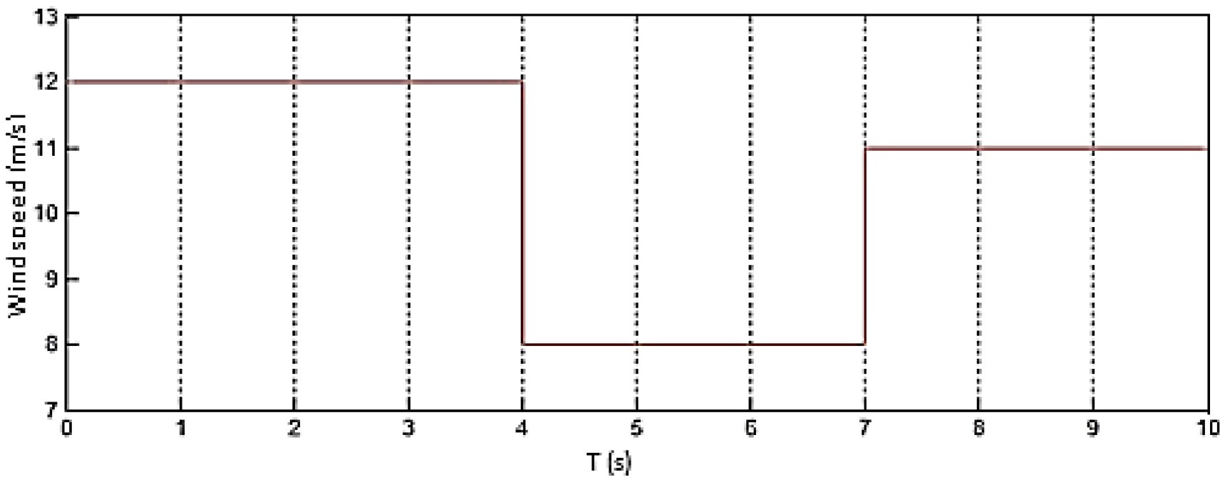
wind speed evolution as a function of time.

Figure 33.

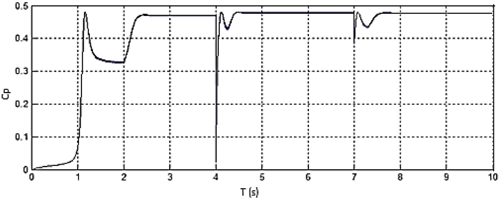
Power coefficient Cp evolution as a function of time.

Figure 34.

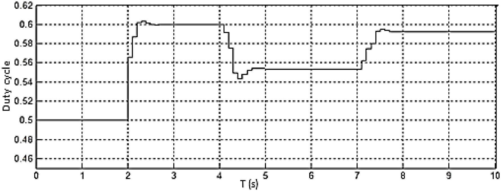
Duty cycle evolution as a function of time.

Figure 35.

Captured electric power evolution as a function of time.

Thus, whatever the wind speed and its amplitude of variation, we manage to capture the maximum possible power for this wind speed. And consequently, we make the most of the energy and economic profit of our installation.

The specification parameters of the turbine are illustrated on Table 2.

Table 2.

Specification of the studied wind turbine.

Parameters	Value
Nominal power	3 KW
Recovered power	2.86 KW
Batteries rated charging voltage	220 V
Internal batteries voltage	210 V
Rectifier delivered power at rated speed	2.891 KW
Turbine efficiency	78%

With the same design and control parameters as used by this study, a study based on an advanced MPPT algorithm leads to similar results to this study (Tounsi, 2022). The strong point of the study presented in this paper is the short simulation time compared to the study already mentioned. What makes the integration of the global system model can be achieved in real time is without sensors.

Experimental test

The energy conversion chain is designed by the analytical method validated by the finite element method. All power chain components manufacturing data is provided by the design model. The control algorithm can be implemented on electronic cards such as DSP or FPGA. In this case, it will be simple to establish a comparative study with a realized prototype.

Conclusion

During this work we were able to optimize the control of a small wind turbine based on PMSG, by designing a system that respects the conditions of simplicity of architecture, cost, and performance and more particularly of energy efficiency.

By exploring the different architectures used in energy conversion chains, we have shown that the most economical structure is that based on a double parallel diode rectifier and a chopper, given the small number of components and the possibility of system control using a single switch.

Simulations results are encouraging and validate completely the design and control approach of WECS.

Footnotes

Appendix

Declaration of conflicting interests

The author declared no potential conflicts of interest with respect to the research, authorship, and/or publication of this article.

Funding

The author received no financial support for the research, authorship, and/or publication of this article.

ORCID iD

Souhir Tounsi

References

Agarwal

Aggarwal

Patidar

, et al. (2010) A novel scheme for rapid tracking of maximum power point in wind energy generation systems. IEEE Transactions on Energy Conversion 25(1): 228–236.

Balasundar

Sudharshanan

Elakkiyavendan

(2015) Design of an optimal tip speed ratio control MPPT algorithm for standalone WECS. International Journal for Research in Applied Science and Engineering Technology 3: 442–450.

Blaabjerg

Chen

Teodorescu

, et al. Power electronicsin wind turbine systems. In: Proc. CES/IEEE Fifth Int. PowerElectron. Motion Control Conf. (IPEMC 2006), Shanghai, China, Aug. 14–16, 2006, pp.1–11.

Dalala

Zahid

, et al. (2013) Design and analysis of an MPPT technique for small-scale wind energy conversion systems. IEEE Transactions on Energy Conversion 28: 756–767.

Gragger

Haumer

Einhorn

(2010) Averaged model of a buck converter for efficiency analysis. Engineering Letter 18(1): 1–6.

Haque

Negnevitsky

Muttaqi

(2010) A novel control strategy for a variable-speed wind turbine with a permanent-magnet synchronous generator. IEEE Transactions on Industry Applications 46: 331–339.

Heydari

Smedley

(2015) Comparison of maximum power point tracking methods for medium to high power wind energy systems. In: Proceedings of 2015 20th Conference on Electrical Power Distribution Networks Conference (EPDC), Zahedan, pp. 184–189. New York: IEEE.

Huang

Jin

(2015) Maximum Power Point Tracking Strategy for large-scale wind generation systems considering wind turbine dynamics. IEEE Transactions on Industrial Electronics [May 1963] 62(4): 2530–2539.

Mahdavian

Wattanapongsakorn

Shahgholian

, et al. (2014) Maximum power point tracking in wind energy conversion systems using tracking control system based on fuzzy controller. In: Proceedings of 2014 11th Inter-national Conference on Electrical Engineering/Electronics, Computer, Telecommunications and Information Technology (ECTI-CON), NakhonRatchasima, May 14–17, New York: IEEE.

10.

Marouani

Tounsi

(2014) Design of a coiled rotor synchronous motor dedicated to electric traction. Journal of Electrical Systems 10(3): 344–358.

11.

Mirecki

(2005) Etude comparative de chaines de conversion d’‘energied’ ediees ‘a une éolienne de petite puissance. PhD thesis.

12.

Nasiri

Milimonfared

Fathi

(2014) Modeling, analysis and comparison of TSR and OTC methods for MPPT and power smoothing in permanent magnet synchronous generator-based wind turbines. Energy Conver. Manag 86: 892–900.

13.

Nasri

Tounsi

(2015) Design and Optimization of Renewable Energy Structure. Journal of Electrical Engineering 7(8): 1–13.

14.

Neji

Tounsi

Sellami

(2006) Contribution à la définition d'un moteur à aimant permanent avec un coût de production réduit pour la propulsion du véhicule électrique. Transactions européennes sur l'énergie électrique (ETEP), Vol. 16, pp. 437–460.

15.

Neji

Tounsi

Sellami

(2006) Contribution to the definition of a permanent magnet motor with reduced production cost for the electrical vehicle propulsion. European Transactions on Electrical Power 16: 437–460.

16.

Pertuza

(1996) Contribution à la définition de moteurs à aimants permanents pour un véhicule électrique routier. Thèse de docteur de l’Institut National Polytechnique de Toulouse, Février.

17.

Rahim

AHMA

(2014) Optimum relation based maximum power point tracking of a PMSG wind generator through converter controls. In: Proceedings of the 7th IET International Conference on Power Electronics, Machines and Drives (PEMD 2014), Manchester, pp. 1–6. New York: IEEE.

18.

Singh

Chandra

(2011) Application of adaptive network-based fuzzy inference system for sensorless control of PMSG-Based wind turbine with nonlinear-load-compensation capabilities. IEEE Transactions on Power Electronics 26: 165–175.

19.

Suilah

Nadia

Boudaya

, et al. (2015) Modelling of Synchronous Generation System for Renewable Energy. International Journal of Electrical Components and Energy Conversion 1(1): 36–43.

20.

Tan

Islam

(2004) Optimum control strategies in energy conversion of PMSG wind turbine system without mechanical sensors. IEEE Transactions on Energy Conversion 19: 392–399.

21.

Tounsi

(2015) Systemic design and optimization improving performances of permanent magnet motors. International Journal of Electrical Components and Energy Conversion 1(1): 1–15.

22.

Tounsi

(2015) Design and optimization of axial flux brushless DC generator dedicated to generation of renewable energy. American Journal of Electrical Power and Energy Systems 4(3): 1–5.

23.

Tounsi

(2022) New approach of maximum power point tracking for wind energy conversion system. Wind Engineering 46(6): 1735–1752.

24.

Tounsi

Neji

Sellami

(2006) Contribution à la conception d’un actionneur à aimants permanents pour véhicules électriques en vue d’optimiser l’autonomie. In: Revue Internationale de Génie Electrique, Vol. 9, 6-2006, pp. 693–718. Édition Lavoisier.

25.

Wei

Zhang

Qiao

, et al. (2016) An adaptive network-based reinforcement learning method for MPPT control of PMSG wind energy conversion systems. IEEE Transactions on Power Electronics 31(11): 7837–7848.