
Abstract
Vibration-based fault diagnostics combined with deep learning approaches has promising applications in detecting and diagnosing faults in wind turbine gearboxes. Specifically when time series vibration data is transformed to a 2-dimensional cyclic spectral coherence maps, the accuracy of deep neural networks in classifying faults increases. Nevertheless, standard deep learning techniques are vulnerable to inaccurate predictions when tested with new data originating from unseen faults or unusual operating conditions. To address some of these shortcomings in the context of wind turbine gearboxes, this paper investigates fault diagnostics using Bayesian convolutional neural network which provide accurate results with uncertainty bounds reducing wrong overconfident classifications. The performance of Bayesian and standard neural networks is compared using a simulation-based dataset of acceleration signals generated from a multibody dynamic model of a 5 MW wind turbine. The framework proposed in this paper has relevance to fault detection and diagnosis in other rotating machinery applications.
Introduction
Among different renewable energy sources, wind energy has grown rapidly in recent years in response to the increase of the global demand for energy and as a replacement of fossil fuels to mitigate the effects of climate change. In 2018, wind energy provided 15% of Europe’s electricity demands (Wind Europe, 2022), and it is expected to supply 20% of the US electricity needs by 2030 (Lu et al., 2009). Wind turbines are typically located in remote regions and are subjected to severe weather conditions, with continually variable loads, wind speeds, and energy demands. As a result, they are prone to failures which results in increasing operation and maintenance costs. According to Verbruggen (2003), operation and maintenance costs account for to 15% of overall cost of energy, with this figure rising to 20%–35% for offshore wind farms. In an effort to lower these costs, more research is done, on the one hand, to improve turbines’ design, manufacturing and materials, and, on the other hand, to improve operational reliability by developing novel fault diagnostic techniques to identify faults early before they worsen and cause substantial damages.
The majority of unexpected downtime and maintenance costs are due to gearbox and generator failures, which account for over 95% of all major replacements in wind turbines (Carroll et al., 2016). Planetary gearboxes are the most commonly used in wind turbines, which, in comparison to fixed shaft gearboxes, offers a high transmission ratio in a more compact package for applications requiring higher output. The trade-off is that they have a higher tendency to fail as a result of their increased workload and more demanding working environment with changing loads and speeds (Feng and Zuo, 2012). According to the National Renewable Energy Lab (NREL), bearings cause 76% of wind turbine gearbox failures, with gear faults being the second most prevalent cause of failure, 17% (Sheng, 2017). Manufacturing and installation issues, design and material defects, misalignment, torque loads, wear and fatigue are all causes of bearing and gear failures.
Examples of gear damage include tooth cracks, abrasion, corrosion, fracture, pitting and scuffing (Qiao and Lu, 2015). According to Yang et al. (2012), if defects are not diagnosed and fixed early, further gearbox deterioration might necessitate replacement of the entire gearbox, which could cost up to $628,000 for a
Vibration-based fault diagnostics for wind turbine gearboxes is the most extensively used approach because of its sensitive and reliable damage detection. The gearbox consists of multiple rotating shafts, sun-planetary gears and bearings. Faults in the gears and bearings manifest themselves in the vibrations, measured through accelerometers, at specific frequencies related to the rotating and gear mesh frequencies (Qiao and Lu, 2015). Several algorithms and signal processing techniques, such as frequency analysis, time synchronous averaging and envelope analysis are used to de-noise the data and extract meaningful information from vibration signals (Sheng, 2012). Each of these methods has its limitations, such as being restricted to cases when the shaft rotational speed is constant. More advanced methods of analyzing vibration data, such as cyclostationary analysis and cyclic spectral coherence (Mauricio et al., 2019) or kurtograms (Antoni, 2007) have been utilized to identify unique fault signatures, that had previously been difficult to diagnose. However, under realistic operating conditions with variable speeds, signal processing techniques alone are insufficient to enable reliable fault diagnostics. Therefore, there has been an increase in the employment of deep learning-based fault diagnosis frameworks, such as convolutional neural networks (CNN), which can automatically and effectively extract the characteristic features related to faults and then use those features to perform detection and classification.
Based on multi-body dynamic modeling and simulations, our work in Amin et al. (2022, 2023b) proposed a deep learning framework that successfully identifies and detects faults with small magnitude located on different gears of the gearbox. Simulations were done under realistic wind conditions, such as turbulent wind, and by including variation in wind speed and loads. Figure 1 describes the flow chart of this simulation-based study using a SIMPACK

An overview of the fault identification framework: Wind turbine loads are applied on the nacelle/drivetrain model and time series accelerometer data is acquired. Synchronous sampling is conducted on acceleration signals before generating cyclostationary maps (images) which are then passed to a CNN for fault diagnosis.
While the results from the CNN models were highly accurate in the aforementioned case study, there are still challenges to be addressed in situations in which this CNN-based framework leads to incorrect classification. One of those challenges is that standard neural networks can be overconfident and produce unreliable diagnostic conclusions when presented with unknown data without offering any warnings. This is due to the frequentist approach that standard neural networks use during training, which limits the learnt model’s parameters or filters to point estimate values, resulting in deterministic outputs for any given input (Shridhar et al., 2019). To address this challenge, we use a Bayesian neural network in this study that considers not only the accuracy, but also the level of confidence or uncertainty in any diagnostic result. With this Bayesian framework, each learnt parameter or weight is represented by a probability distribution as opposed to a single value, which allows for the evaluation of certainty of each classification result.
Multi-body dynamic modeling and simulations
Flexible multibody dynamics is a field that deals with using computers to model and analyze the behavior of bodies that are both deformable and constrained, and which undergo significant displacement and rotation. In a flexible multibody system, there may be a combination of rigid and elastic components, connected by joints or force elements such as springs, dampers, and actuators. Because of the constraints imposed by the joints, the movements of the bodies within the system are not entirely independent. The nonlinear nature of the governing dynamic equations of motion and the high dimensionality of flexible multibody systems necessitate the use of computer software that employs numerical algorithms to solve the equations of motion and analyze the system’s behavior (Shabana, 1997; Simeon, 2013).
SIMPACK is a dynamic analysis tool that uses multibody simulation to examine the response of drive systems. It takes into account the behavior of rotating machinery such as gears, bearings and more, by modeling them with the use of springs and dampers. For wind turbines, SIMPACK incorporates the structural flexibility of the drivetrain components like the bed-plate, gearbox housing, and shafts, by utilizing the Craig-Bampton finite element method (Guo and Keller, 2018). An onshore 5 MW three-blade turbine model is represented by the SIMPACK multi-body model in Figure 2. Drivetrain components are housed inside the nacelle, which is mounted to the top of the tower.
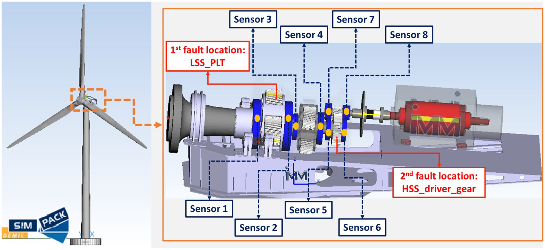
Full onshore wind turbine model, hub and nacelle. Screenshot images from the SIMPACK model are taken by the author.
An input main shaft, a three-stage planetary gearbox, a high-speed coupling that connects to the generator, a main frame, a housing, and a yaw bearing make up the drivetrain. The high-speed shaft (HSS) drives the electrical generator, while the low speed shaft (LSS) attaches the rotor hub to the gearbox. The gearbox model comprises of a flexible main shaft and flexible housing with three active dynamic modes. Eight accelerometers, labeled 1 through 8 in Figure 2, are embedded in the drivetrain model to measure and collect accelerations at different bearing locations on the gearbox. To more accurately model the gear tooth contact and to account for the forces and moments generated in the gear mesh, this SIMPACK model incorporates a high-fidelity gear force element into all gears. All gearbox element details, the calculated rotating and gear mesh frequencies are detailed in Amin et al. (2023a, 2023b), with a final gear ratio of 97.83.
An interface to the wind load simulation program AeroDyn in SIMPACK was utilized to represent the wind loads in full wind turbine simulations performed under nine different wind conditions and speeds, with the gearbox remaining in healthy condition (Jonkman, 2009; Jonkman et al., 2015). Among the nine simulated scenarios, there were three cases of turbulent wind, two events of laminar flow, one instance of an extreme operating gust, two instances of extreme direction changes, and one wind speed run-up scenario with noise. Figure 3 shows examples of the wind speed profile for each of the simulated wind scenarios. After that, wind loads, speeds, and torques are extracted from each scenario and applied to the abstracted nacelle only model to simulate the loads given by wind turbine blades in an experimental configuration. The frequency spectrum of the high dynamic forces and moments created by the blades is often in the low frequency domain, as detailed in our study (Amin et al., 2022), making low-speed stage (LSS) problem diagnostics more difficult.
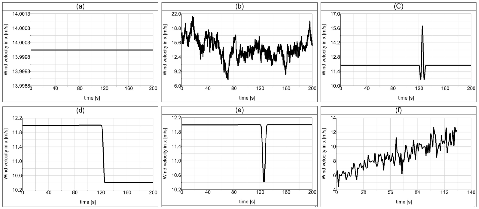
Example of simulated wind conditions: (a) laminar wind, (b) turbulent wind, (c) extreme operating gust, (d) extreme direction change, (e) twice extreme direction changes, and (f) run-up 6–12 m/s with random noise.
To simulate the presence of a localized fault or a crack on gears, a tooth pitch error is introduced into the model. On the low-speed planetary stage, the first simulated fault is created on one of the planet gears (LSS). The second fault, shown in Figure 2, is on the driver high speed shaft (HSS) gear. These faults cause periodic impulses or modulation phenomena in the vibration signal, and the corresponding characteristic frequency is linked to the rotating frequency of the damaged gear. To reflect variations in the severity level, fault size change is reflected by altering the magnitude of each fault, ranging from 100 to 50 and finally down to 20 μm. A single tooth on one side of the respective gear wheels is affected by the fault. Because either of the two faults were present in every simulation, they did not exist concurrently in this study. To classify and detect the fault on the LSS, vibration signals from sensors 1 to 4 are selected from the simulation data. The final four sensors, numbered 5–8, are used to classify the HSS fault.
Cyclostationary analysis
A signal is considered to be cyclostationary of order

Since the autocorrelation function

where

Using equation (3), we can derive the spectral correlation function

where

A bivariable map, based on
In our gearbox dataset, HSS fault signature occurs at 4.7 cycle/rad which can be clearly identified using cyclic spectral coherence (CSCoh) maps. As show in Figure 4(a), the fault signature of HSS 100 μm is strong and very clear at 4.7 cycle/rad. As the fault magnitude is small or at an early stage, the signature gets weaker, as shown in CSCoh map for the HSS 20 μm fault in Figure 4(b). Additionally, the y-axis carrier frequency range decreases as fault magnitude decreases. So, the larger the amplitude of the fault, the broader the spectrum of frequencies it excites.
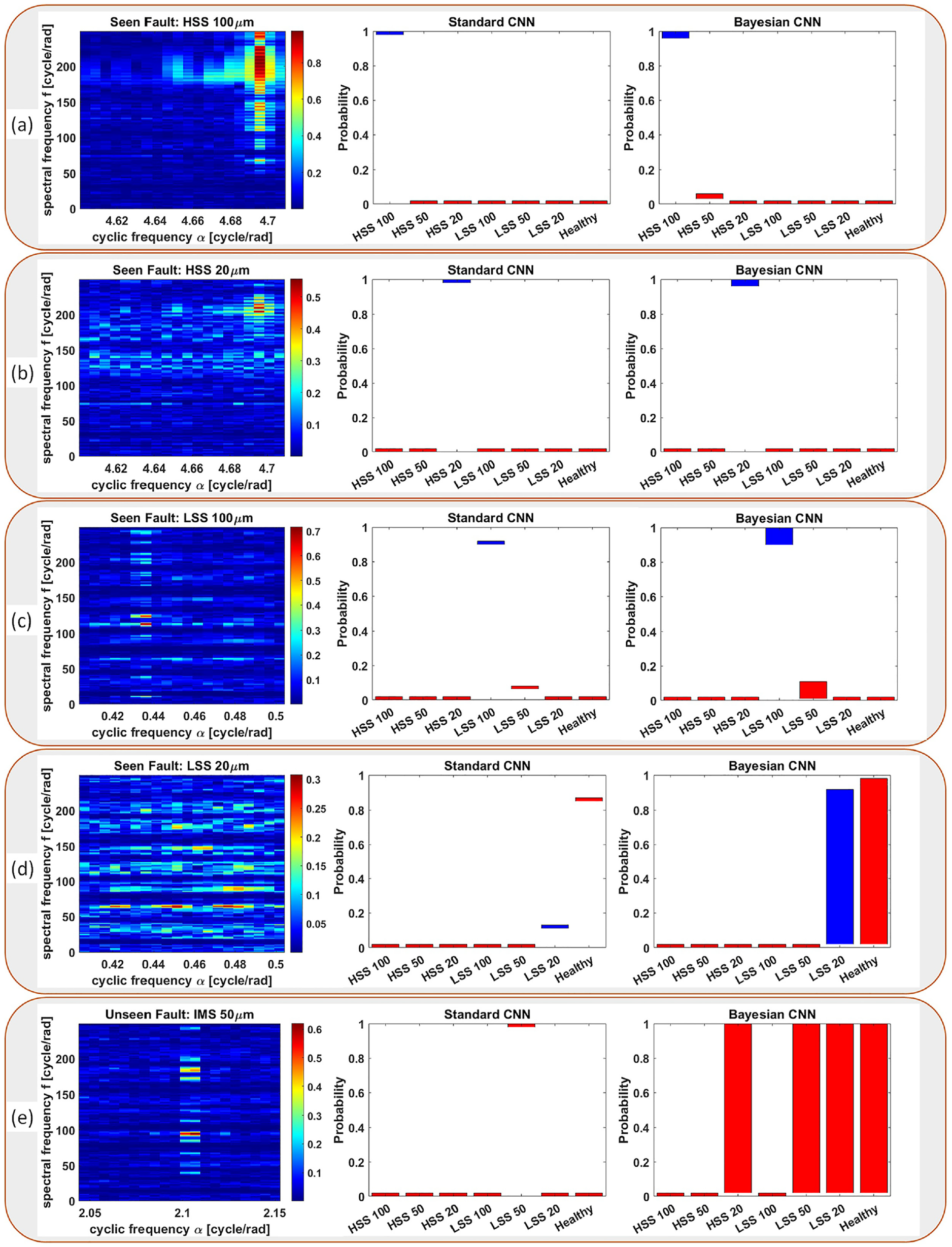
Comparison of diagnostic results between Standard and Bayesian Convolutional Neural Networks using cyclic spectral coherence maps of vibration signals. Cases (a–d): seen faults on HSS and LSS. Case (e): unseen fault on IMS. BCNN predictions are plotted with a 95% confidence interval and are accompanied by their corresponding true labels in blue, while incorrect labels are displayed in red. Training and testing images provided to the neural network were devoid of any labels, axis numbers, or colorbars.
However, the LSS fault signature is only discernible on CSCoh maps when the fault magnitude is large, such as LSS 100 μm fault. As seen in Figure 4(c) and (d), as fault size decreases, the signature at 0.44 cycle/rad frequency becomes less distinct and harder to trace. These example plots in Figure 4(c) and (d), were generated using data from sensor 1, which is physically located closest to the damage. Sensors 3 and 4, which are further away from the damage, exhibit a weaker signature. Moreover, the spectral/carrier frequency range for the fault is narrower compared with HSS fault. This motivates the use of convolutional neural networks (CNN) for precise defect identification, which is detailed in Amin et al. (2023a, 2023b).
Bayesian convolutional neural network
A convolutional neural network (CNN) is often used in image recognition for damage classification (Jing et al., 2017). A CNN is capable of identifying spatially local correlation features in an image. The performance of CNN depends on the convolution operation for feature extraction and pattern recognition. Typical CNN architectures include four types of layers: a convolutional layer, a pooling layer, a Rectified linear unit (ReLU) layer, and a fully connected layer (Guo et al., 2018). In Amin et al. (2023a), we employed a CNN model trained on cyclic spectral coherence (CSCoh) images to perform fault diagnostics on the two faults introduced into our gearbox model. This conventional CNN works by optimizing a loss function to determine the best model parameters based on a known training data. In machine learning, the loss function serves as a measure of the error or discrepancy between the predicted output and the actual target to quantify how far off the model’s prediction from reality. The goal is to typically minimize this loss value. Adam, an adaptive moment estimation optimizer, is used to optimize a cross-entropy loss function that is then used to provide classification results. A Cross-Entropy loss is often used in classification tasks to quantify the dissimilarity between the predicted probabilities and the true categorical labels (Zhang and Sabuncu, 2018). A maximum likelihood estimation (MLE) is used to determine model parameters, weights, and biases; as a result, these parameters can only have single deterministic values (Blundell et al., 2015). For a set of training data

This approach is effective if the testing data follows the same distribution of the training data. Specifically, if we keep testing images from fault-free cases and the two simulated damaged cases in our gearbox model. This is referred to as the in-distribution dataset. However, the inability of expressing uncertainty in the output is a drawback of this CNN-based approach (Jospin et al., 2022; Shridhar et al., 2019). Another issue is that it is highly unrealistic and unlikely for the test data to have the same distribution as the training data. This is due to the fact that it is extremely challenging to gather training data for each and every potential event or failure mode that may occur in the gearbox operating in the field. As a result, any out-of-distribution testing, such as the existence of new faults that were unknown during training, would result in meaningless or wrong overconfident predictions from this traditional CNN-based framework (Jospin et al., 2022). For instance, the CNN has been trained to accurately diagnose faults on LSS and HSS. Any unseen fault, say on the intermediate speed shaft (IMS), will be blindly diagnosed into any of the existing LSS and HSS faults. This means that the network would still assign a category to any new input image even if it is unrelated to what it has been trained on. Such untrustworthy results fail to meet the reliability and safety requirements for accurate fault diagnosis.
The challenges with conventional CNNs can be resolved by utilizing a Bayesian neural network (BNN), in which a probability distribution is learnt across all model parameters, that is, weights and biases. This gives it advantages to capture prediction uncertainty. In addition, BNNs are considered to be highly data-efficient, allowing them to effectively learn from small datasets without the risk of overfitting (Depeweg et al., 2018). This property makes BNNs particularly well-suited for the kind of simulation dataset that we are working with, which may be limited in size or scope. By utilizing a probabilistic approach to learning, BNNs are able to better model the inherent uncertainty in small datasets, which results in more robust and accurate predictions. This advantage can be especially important in scientific or engineering applications where data collection may be difficult or time-consuming. Moreover, BNNs are often considered to be a special case of ensemble learning (Jospin et al., 2022). In effect, BNNs generate a family of models that represent different possible ways of fitting the data, rather than relying on a single best-fit model. This approach is similar to ensemble learning, where multiple models are trained, and their outputs combined to improve performance. However, BNNs differ from traditional ensemble methods in that they generate a distribution of models from a single training process, rather than training multiple models independently.
As previously stated, the probabilistic approach used by BNNs involves learning a probability distribution, known as a variational posterior, over the model parameters both during training and after examining the training data. This is done using the Bayes’ theorem to find the posterior distribution

where

where the function
Variational inference
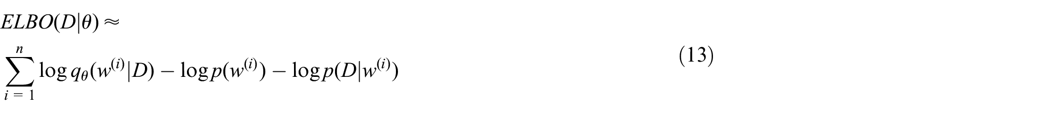
The difficulty in computing the complex posterior distribution is addressed by proposing a method based on the variational inference technique known as Bayes through Back-propagation (Shridhar et al., 2018). This method aims to approximate the true posterior distribution by using a computationally tractable approximation. This done by using a known distribution, specifically called variational posterior

In this expression the weights


where

where
where
Uncertainty in Bayesian neural network
A key benefit of Bayesian neural networks compared to standard frequentist neural networks is their capability to quantitatively express uncertainty. When doing classification tasks, we are interested in the predictive distribution

As explained in Variational Inference subsection, Gaussian distributions

with
On real data, however, there is no conjugacy between categorical and Gaussian distributions. Thus, a closed form solution to equation (15) does not exist. Nevertheless, by sampling from the variational distribution
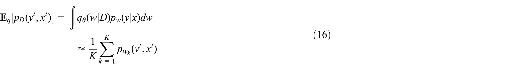
where

This variance quantifies the amount of uncertainty or randomness in the model’s output, indicating how much the predicted result may deviate from the true value. Essentially, a low variance in the estimator indicates that the network is highly certain in its prediction, while a high variance reflects a greater degree of uncertainty. Understanding the variance of this estimator is essential for gauging the reliability of the network’s predictions. A confident prediction should have a high mean predictive probability and a low variance value. The derivation of these equations is further explained in Shridhar et al. (2019, 2018).
Fault diagnostics using deep learning
This section discusses the implementation of the proposed BCNN and draws comparisons to the results obtained by using a standard CNN on our simulated-based gearbox dataset. There are two types of faults, each of which can occur at one of three possible severity levels (100, 50, or 20 μm) in addition to the healthy case. This gives us a total of seven categories for classifying results. Figure 4 presents examples for CSCoh maps of some simulated faults, followed by visualizations of predictions using standard CNN and BCNN. A total of 276 coherence intensity matrices for all images with the size of
Standard convolutional neural network
The used CNN architecture contains three 2D convolution layers and three 2D pooling layers: 20
Bayesian convolutional neural network
The used BCNN architecture is similar to the standard CNN with each parameter represented by a normal distribution as shown in Figure 5(a). Thus, the mean and standard deviation of each weight and bias is learnt during training. The learning rate of 0.01 used in the standard CNN is also employed here. The obtained accuracy level was 90%. As explained in 4.2, the weights in a BCNN are not fixed but instead are represented by a learned probability distribution. To make a prediction using the BCNN, we need to generate multiple samples or run the network several times for each input image as depicted in Figure 5(b). Since the model parameters are being sampled each time, each prediction is likely to be slightly different. In our model, we used a predefined
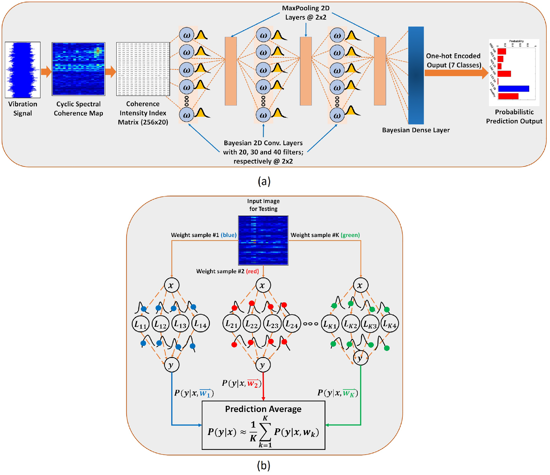
(a) A workflow to implement, train and evaluate the Bayesian Convolutional Neural Network on vibration raw data represented by cyclic spectral coherence maps. (b) An uncertainty-aware prediction for a given input image by drawing
If we examine the BCNN prediction in Figure 4, we see that it is just as accurate as the conventional CNN in cases (a) and (b). In case (c), which is for LSS 100 μm, as explained earlier the fault signature is weaker compared to the HSS. This is reflected by a marginal increase in the height of the bar, indicating a higher level of uncertainty for this class prediction. In scenario (d), the BCNN still gives a larger probability to the healthy class than the LSS 20 μm class, but the level of uncertainty is substantial, as seen by the extreme differences in bar heights. Out of the 100 samples, the output was almost 0.01 in one sample and nearly 0.98 in another for the healthy class. This means that the diagnostic result is untrustworthy and should be investigated further. Case (e) is an example where the BCNN model demonstrates that it has tested something new, as evidenced by the wide probability distribution allocated to the four classes with a significant degree of uncertainty. To avoid incorrect classification, the BCNN here tries to communicate that it is unsure about any category it has not seen or trained on before.
Figure 6 provides a closer look at the probability predictions for the first four images shown in Figure 4. The y-axis of the scatter plots displays the probability of correct predictions for each of the four cases: HSS 100 μm, HSS 20 μm, LSS 100 μm, and LSS 20 μm; respectively. As previously noted, the Bayesian neural network (BNN) produces highly accurate and confident results for cases (a), (b), and (c). However, for the last scatter plot, case (d), the 100 samples from the trained BNN assigned widely varying probabilities for the LSS 20 μm class, ranging from 0 to 1. This indicates a high level of uncertainty in the prediction, as also shown by the large height of the corresponding bar in Figure 4(d). The standard deviation for the first three tested cases is zero, while the fourth case has a standard deviation of
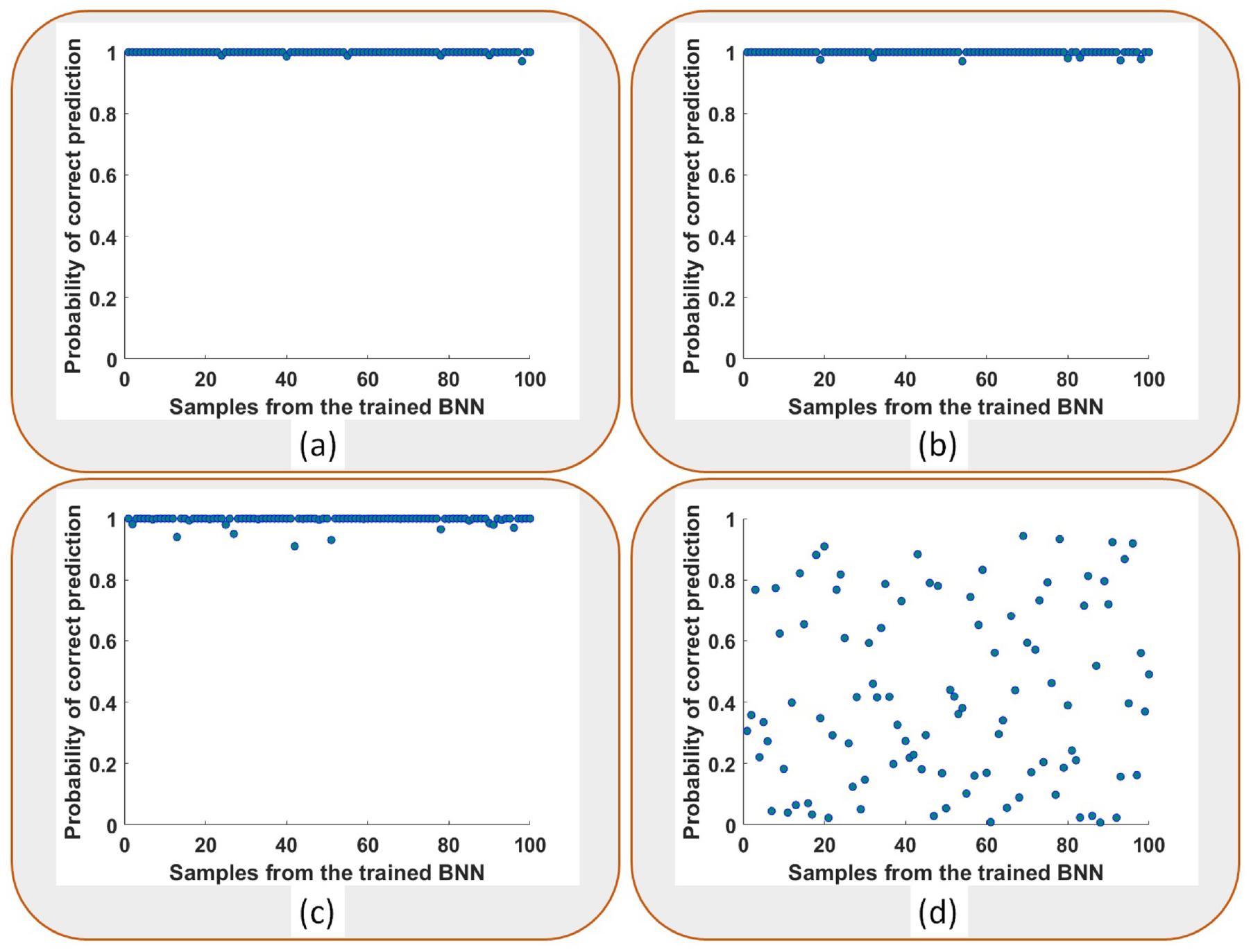
Bayesian neural network probabilistic results from drawing 100 samples for each test image of seen faults (a) HSS 100 μm, (b) HSS 20 μm, (c) LSS 100 μm, and (d) LSS 20 μm.
Conclusion
In this study, the performance of vibration-based fault diagnostic systems employing Bayesian and traditional neural networks is compared and assessed. Using simulation-based dataset, the Bayesian neural network can provide the level of uncertainty in the classification results. Since the level of uncertainty is minimal while dealing with HSS faults, the performance of the two networks, BCNN and standard CNN, is very similar. For the LSS fault, however, the impact signature is negligible at low fault magnitudes. Therefore, the level of uncertainty is higher in this case, which is solely represented in the BCNN’s results in Figure 4(c) and (d). When tested with an unknown fault type, such an IMS fault, the BCNN obviously indicates its degree of doubt about the new pictures by assigning equally distributed predictions over four different classes. This simply means the network is stumped on identifying the new image and requires human intervention for further investigation. In contrast to the BCNN, when tested with this IMS fault type, the standard CNN assigned a completely wrong overconfident classification, claiming instead that the fault is LSS 50 μm as shown in Figure 4(e). This research creates a more comprehensive framework for the application of deep learning algorithms to ensure the safety and reliability of wind turbine fault diagnostics. The Bayesian neural network serves to round out this strategy considering both the accuracy and trustworthiness or the level of confidence of the diagnostic results.
Footnotes
Declaration of conflicting interests
The author(s) declared no potential conflicts of interest with respect to the research, authorship, and/or publication of this article.
Funding
The author(s) received no financial support for the research, authorship, and/or publication of this article.