
Abstract
One of the fundamental aspects essential for ensuring the steadiness of wind power generation and the management of power systems is the accurate forecast of wind speed. We propose a short-term wind speed prediction model based on decomposition and bidirectional long short-term memory network. Firstly, the short-term wind speed is input into complete ensemble empirical mode decomposition of adaptive noise processing, which decomposes it into components with different local characteristic information to decrease the complexity of the wind speed pattern. Then, the bidirectional long short-term memory network with the attention mechanism is fitted with the decomposed data, and the particle swarm optimization algorithm is selected to optimize the hyper-parameters of bidirectional long short-term memory network to reduce the errors in modeling process. To derive the final prediction results, the forecasted values of each model output are added. The experimental results of two real short-term wind speed datasets verify that the designed approach has high accuracy in short-term wind speed forecasting, and its prediction values are better than other comparison models.
Keywords
Introduction
For wind power generation scenario, energy storage faces the dilemma with high difficulty and high cost. Most generators adopt linear conversion architecture with direct source acquisition and direct terminal power supply. In addition, wind power integration is a major challenge for wind power generation (Shahid et al., 2023). During the peak period of power consumption, the access of a large number of intermittent energy sources will affect the frequency modulation range of power, resulting in power instability (Kumar et al., 2025).
Considering different prediction time, the prediction problem of wind speed can be divided into short-term prediction, medium-term and long-term. The long-term prediction mainly focuses on the general change trend of annual wind speed in the future with year as the time scale, and its forecast results can provide scientific support for the location decision of wind farms. The medium-term forecasting covers the wind speed from weeks to months in the future, which is the key basis for wind farm power generation planning. The short-term forecasting focuses on the wind speed changes in the next few minutes to hours, which can directly assist the real-time operation regulation of wind turbines. Therefore, it is very worthwhile to study the prediction index of improving short-term wind speed for power system scenarios (Dhaka et al., 2024).
At present, many achievements of short-term wind speed prediction have been reported, including physical models, artificial intelligence models, statistical models and combined prediction models (Tian et al., 2025). On the basis of real-time information such as on-site wind speed, wind direction and numerical weather prediction, physical models are usually estimated by solving N-S equations (Yang et al., 2025a). The artificial intelligence model is considered to be composed of deep learning model and machine learning model. Machine models such as random forest and support vector regression use the nonlinear relationship between wind speeds to obtain models. The statistical models predict wind speed based on historical statistical data. The combined prediction model considers the prediction effect of a single model. On the basis of the forecasting values of different approach, a statistical analysis model is established to integrate or weight each prediction model.
At present, many of the deep learning-based approaches are applied to the forecasting of short-term wind speed. Long Short-Term Memory (LSTM) network is chosen as forecasting model, and the results showed that the LSTM is superior to other methods (Huang et al., 2021). But the model complexity of LSTM network is high and the training time is relatively high. Aiming at decrease the complexity, Adam et al. proposed a deep learning frame based on Gated Recurrent Unit (GRU), and a comparative study between it and LSTM network found that the GRU is superior to the LSTM in accuracy and training time (Adam et al., 2021). Although each method has an adaptive scenario, it is often a challenge to make a single model produce the best prediction. Mohammed and Mohammed constructed a Convolutional Neural Network prediction model based on GRU network (CNN-GRU), where the convolutional layer extracts the data features to improve the forecasting accuracy, while the gated recursive unit stores the information in memory. The comparison results show that the CNN-GRU is superior to other benchmark approaches (Mohammed and Mohammed, 2022). However, the GRU network needs to adjust too many hyper-parameters when dealing with different types of data.
Many combined models are a combination of decomposition algorithms with multiple models to forecast short-term wind speed. The advantages of each model or algorithm are fully utilized to improve the accuracy of prediction. Han et al. used LSTM combined with Variational Mode Decomposition (VMD) for modeling and found that the forecasting accuracy of wind speed was significantly improved after VMD processing (Han et al., 2019). However, the computational complexity of VMD is high, especially for signals with long time series, and the computation time may be long. Liu et al. applied Empirical Modal Decomposition (EMD) to decompose the short-term wind speed and subsequently uses neural network for prediction. Their achievements increase the convenience of prediction and enhance the accuracy of prediction (Liu et al., 2013). However, the EMD method is prone to modal aliasing or endpoint effects. He and Wang combined the improved Ensemble Empirical Mode Decomposition (EEMD) with the least absolute shrinkage and selection operator-quantile regression neural network model to overcome the modal aliasing problem and enhance the prediction accuracy (He and Wang, 2021). However, there may be interference noise in the decomposition sequence, which affects the prediction accuracy. Aiming at suppress noise, Xiong et al. introduced Complete Ensemble Empirical Mode Decomposition (CEEMD) to decompose the wind power samples, which effectively eliminates the interference noise in the decomposed sequence, thus improving the fitting degree of prediction (Xiong et al., 2023). However, the disadvantage of CEEMD is that if the added white noise amplitude and the number of iterations are not properly selected, redundant IMF components are generated, which need to be restructured or processed.
In our study, the original short-term wind speed samples are handled with Complete Ensemble Empirical Mode Decomposition with Adaptive Noise (CEEMDAN). During the decomposition process, the final reconstructed signal has less noise residue than the EEMD result, thus minimizing the number of screenings. This is achieved by summing the IMF components of each order resulting from the white noise EMD decomposition. The decomposed components are input into the Bidirectional Long Short-term Memory (BiLSTM) model with attention mechanism (BiLSTM-Attention) for forecasting. BiLSTM-Attention can not only capture long-term dependencies on historical time steps in the sequence, but also handle importance based sampling. Meanwhile, the Particle Swarm Optimization (PSO) algorithm optimized the hyper-parameters of the BiLSTM-Attention model to reinforce the forecasting index. Simulation comparisons demonstrate the great forecasting index of the approach presented in this research. The main innovative work is as follows. 1. CEEMDAN is adopted to decompose short-term wind speed samples, reduce the complexity of original data, and is more conducive to the prediction of prediction models. 2. The attention mechanism is introduced into the BiLSTM-Attention model, which can capture the long-term dependence on the historical time step in the sequence, and can process the importance-based sampling information. 3. The PSO algorithm is used as optimization strategy to determine the hyper-parameters of the BiLSTM-Attention model to reduce forecasting error.
The other contents of this study are arranged as follows. Section 'Basic theory' gives the principles of CEEMDAN algorithm, BiLSTM with the attention mechanism, PSO algorithm and hyper-parameter optimization of BiLSTM. Section 'Designed prediction model' presents the implementation process of the designed prediction model. The effectiveness of the designed approach is validated in Section 'Case studies'. Section 'Conclusion' introduces the conclusions and future work.
Basic theory
CEEMDAN algorithm
CEEMDAN draws on the idea of EEMD algorithm, adds Gaussian white noise to it, and performs multiple superposition averaging on the basis of EMD improvement, so as to achieve the effect of removing noise (Li et al., 2025). It successfully solves the problem of excessive average time of EEMD algorithm and improves the decomposition efficiency of the algorithm. The CEEMDAN algorithm can be described as follows:
1. For original short-term wind speed signal

2. New generated signal sequence


3. After adding white noise


4. According to equation (6), the original short-term wind speed signal is processed and the above steps are repeated. Additional white noise decomposition is performed each time until the resulting residual cannot be further decomposed.

BiLSTM with the attention mechanism
Standard LSTM can only mine the feature information of time series data that has appeared in the past, but cannot mine the information of time series data that has never appeared, so the learning efficiency is low and the prediction accuracy is low. BiLSTM can not only use the information of past time samples, but also learn understand the features of future samples by bidirectional mining the information of time series data, which enhances the model’s utilization of samples and makes the learning ability better (Lu et al., 2025; Zhu et al., 2025). The frame of BiLSTM is shown in Figure 1. Frame of BiLSTM.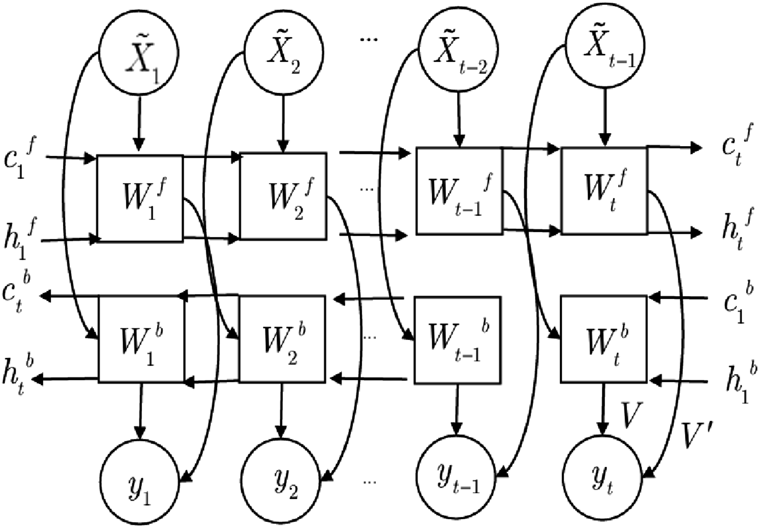
The attention mechanism is a way for neural network to concern on significant portion of the input data. When dealing with input samples, the attention mechanism can process the most relevant data by assigning a weight to each input time point (Wu et al., 2026). In this way, even in the case of missing or abnormal data at some time points, the BiLSTM can make accurate forecasting.
Adding an attention layer to the BiLSTM model structure is the basic principle behind the BiLSTM-Attention model. This makes it possible for the attention layer to sample the input time series data to determine its importance, and then input the importance sampling data as input data into the BiLSTM model for training, modeling and prediction. The BiLSTM-Attention model can not only deal with importance-based sampling, but also deal with the long-term dependence of sequences on historical time steps. The BiLSTM in Figure 1 introduces the attention mechanism by defining an attention layer, where the attention layer weight is denoted by W,
PSO algorithm
Some hyper-parameters in the BiLSTM can affect the prediction accuracy of the model, such as regularization parameters, learning rate, number of training iterations, batch size and the number of neurons, etc. (Li et al., 2022). The optimization algorithm can be applied to optimize the above hyper-parameters. As a classical optimization algorithm, PSO algorithm has achieved excellent performance in many fields.
As a swarm intelligence algorithm, PSO is come from the foraging behavior of birds (Alhussan et al., 2023; Priyadarshi and Kumar, 2025). The problem of finding food for birds in one-dimensional space is extended to multidimensional space. Suppose in a K-dimensional space, the position of a particle is denoted by


Hyper-parameter optimization of BiLSTM
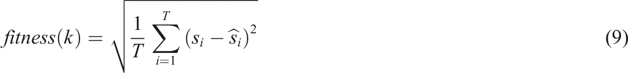
The foreasting accuracy of BiLSTM model is closely related to the values of hyper-parameters. At present, the values of hyper-parameters are mostly based on experience, and sometimes even through multiple trials to achieve better prediction accuracy. The PSO algorithm has significant advantages in computing such complex problems due to its powerful optimization ability and fast convergence speed. PSO algorithm is determined to optimize the hyper-parameters of the BiLSTM. For the BiLSTM model, parameters such as the number of memory units and dropout rate do have a consequence on the capability of the network such as accuracy and generalization ability. But their impact is not as significant as the learning rate, the number of hidden neurons and the batch size. Klaus et al. has pointed out that the learning rate, the number of hidden neurons and batch size are the main hyper-parameters that have greatest impact on the prediction performance of BiLSTM (Klaus et al., 2017). Many studies also optimize these three parameters (Qiao et al., 2023; Yang et al., 2025b). The intervention of PSO is not conducive to the complexity of the model, and the number of optimization variables is also related to the time cost of the model. Based on the above considerations, this paper chooses PSO to process the three parameters of learning rate, number of hidden layer neurons and batch size. Figure 2 provides the specific optimization process. Flowchart of PSO optimized BiLSTM-Attention.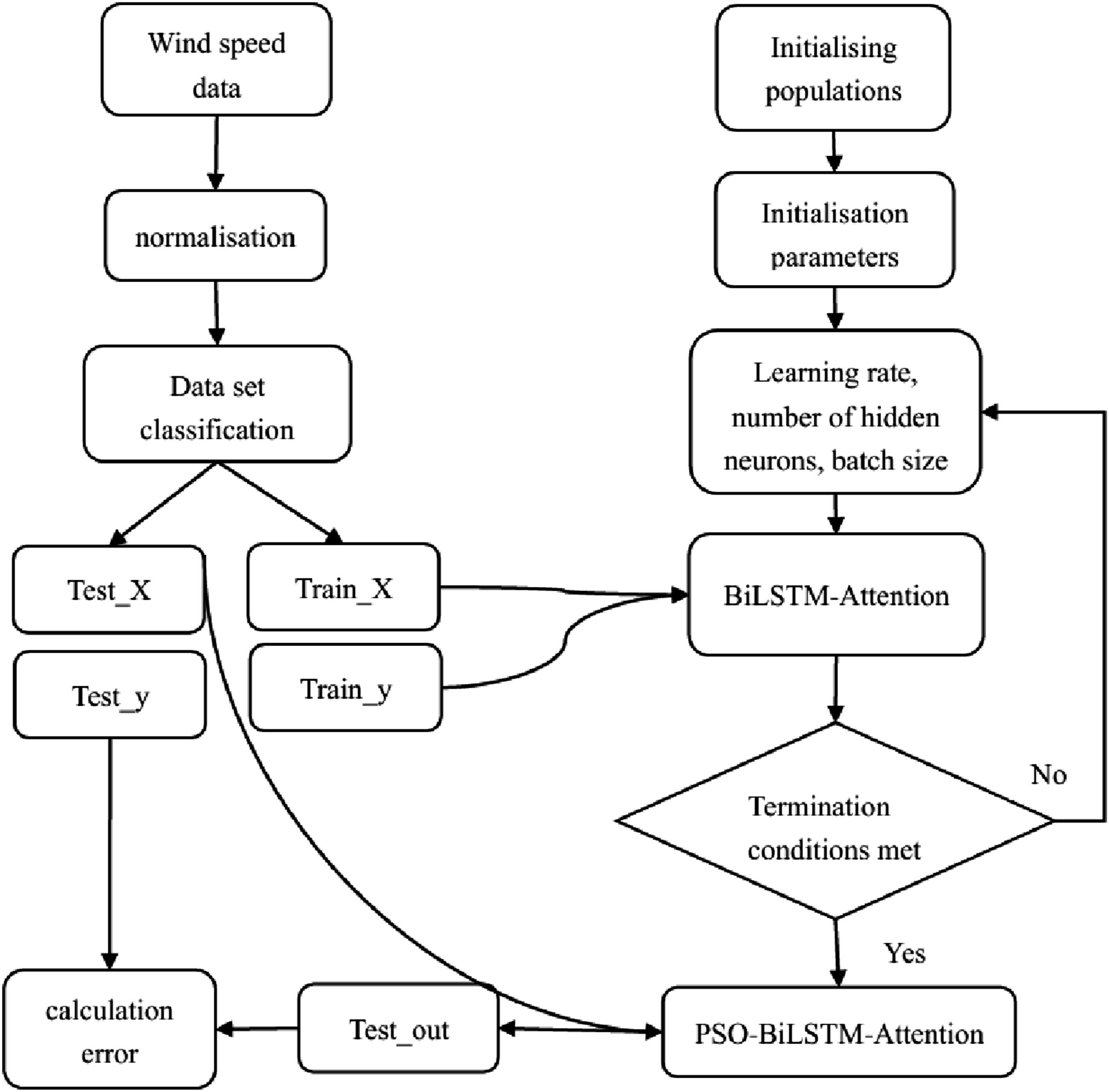
The implementation process of PSO optimized BiLSTM-Attention is introduced as follows.
Designed prediction model
The flowchart of the designed CEEMDAN-PSO-BiLSTM-Attention is shown in Figure 3. Flowchart of designed short-term wind speed prediction model.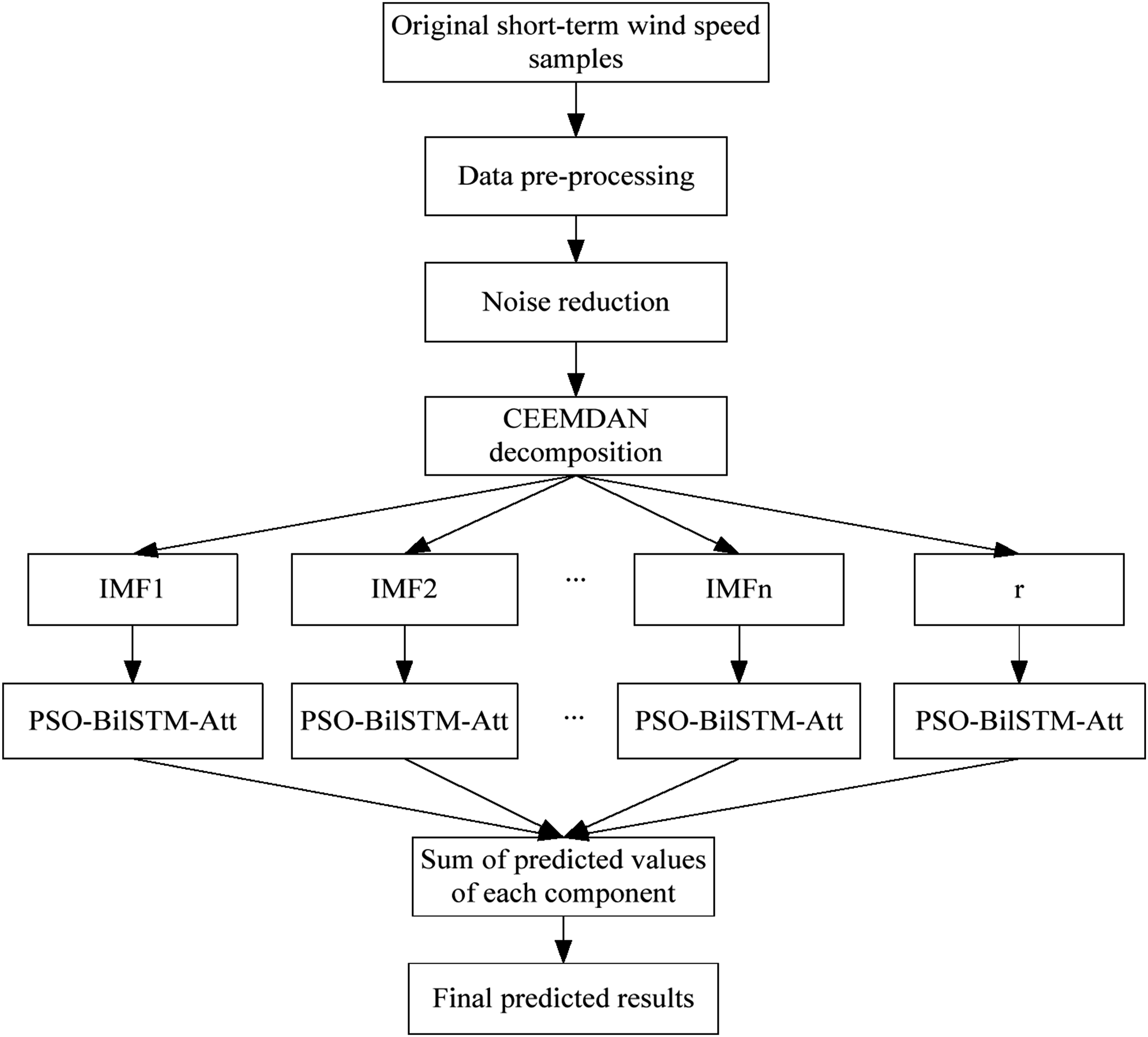
The specific process of the model can be described as follows.

Case studies
Datasets
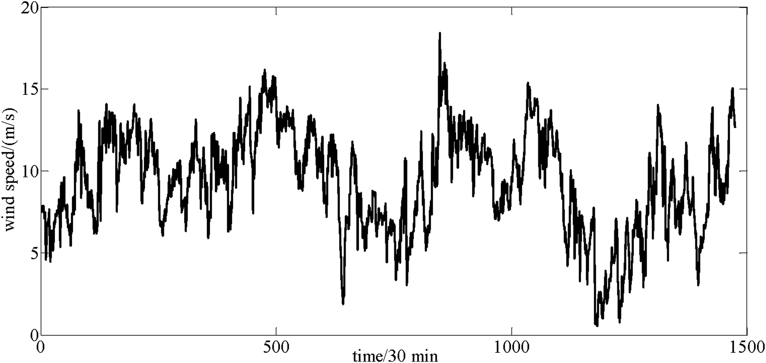
The data of the study come from wind turbine SCADA in Turkey in 2018, which is divided into dataset A and dataset B according to the sampling interval. The data source is https://www.kaggle.com/datasets/berkerisen/wind-turbine-scada-dataset?resource=download. In dataset A, the collection period is from 00:00 on 1 February 2018 to 23:50 on 28 February 2018, the sample size is 4463, and the sampling period is 10 minutes. In dataset B, the collection period is from 00:00 on 1 August 2018 to 23:30 on 31 August 2018, the sample size is 1488 and a sampling period of 30 minutes. The training set and test set are designed based on the principle of 8:2. The number of training sets of dataset A is 3570, the number of test sets is 893, the number of training sets of dataset B is 1190, and the number of test sets is 298. The original wind speed sample is displayed in Figures 4 and 5. Original short-term wind speed of dataset A. Original short-term wind speed of dataset B.
The operating system used in the experiment is Windows 10, and Anaconda is used to build the virtual environment required for the experiment. The framework used for the model is Pytorch, and the experimental code development platform is Jupyter Notebook. The GPU model is NVIDIA GeForce MX250, the CPU model is Intel (R) Core (TM) I5-10400H 2.6 GHz, the memory is 16 GB, and the video memory is 6 GB.
CEEMDAN decomposition and comparison
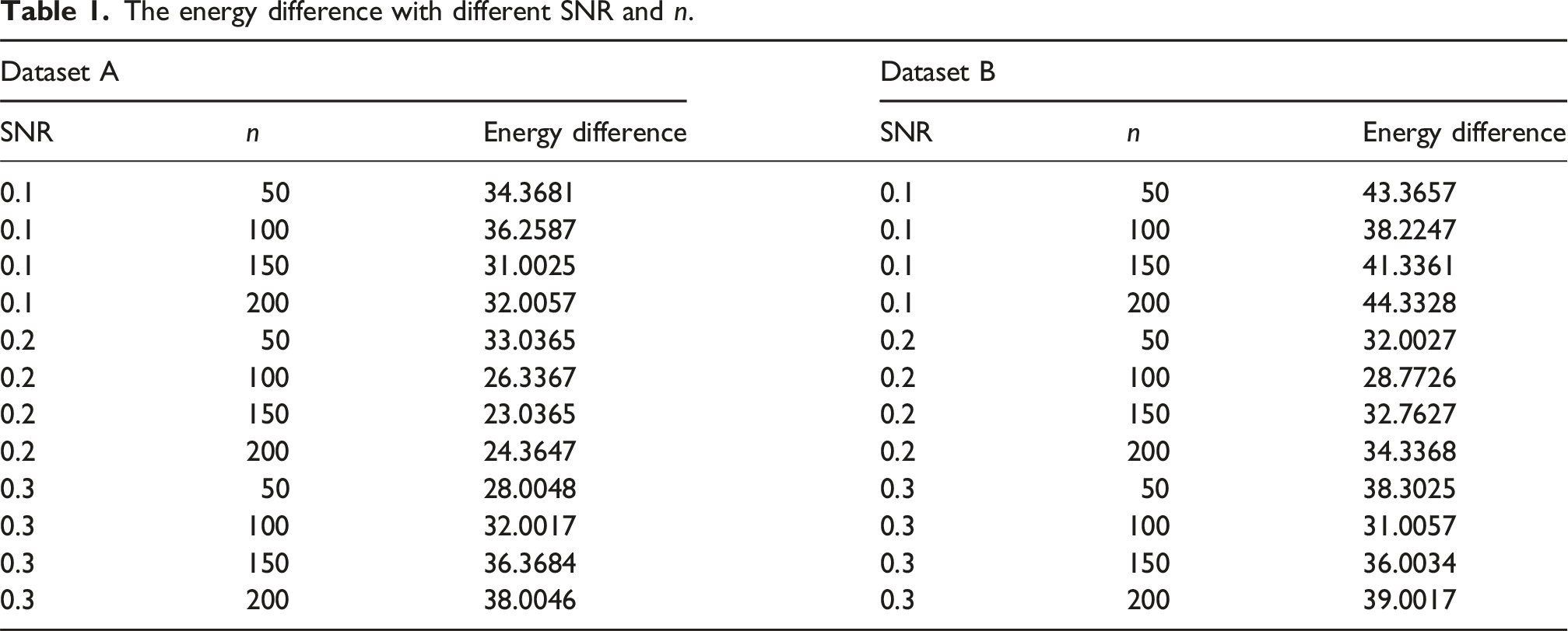
The energy difference with different SNR and n.
To verify the performance of the CEEMDAN decomposition algorithm, a comparison is made with two decomposition algorithms, EMD and EEMD. Figures 6–8 respectively show the decomposition effects of EMD, EEMD, and CEEMDAN on dataset A. Similarly, Figures 9–11 show the decomposition effect on dataset B. EMD decomposition results (dataset A). EEMD decomposition results (dataset A). CEEMDAN decomposition results (dataset A). EMD decomposition results (dataset B). EEMD decomposition results (dataset B). CEEMDAN decomposition results (dataset B).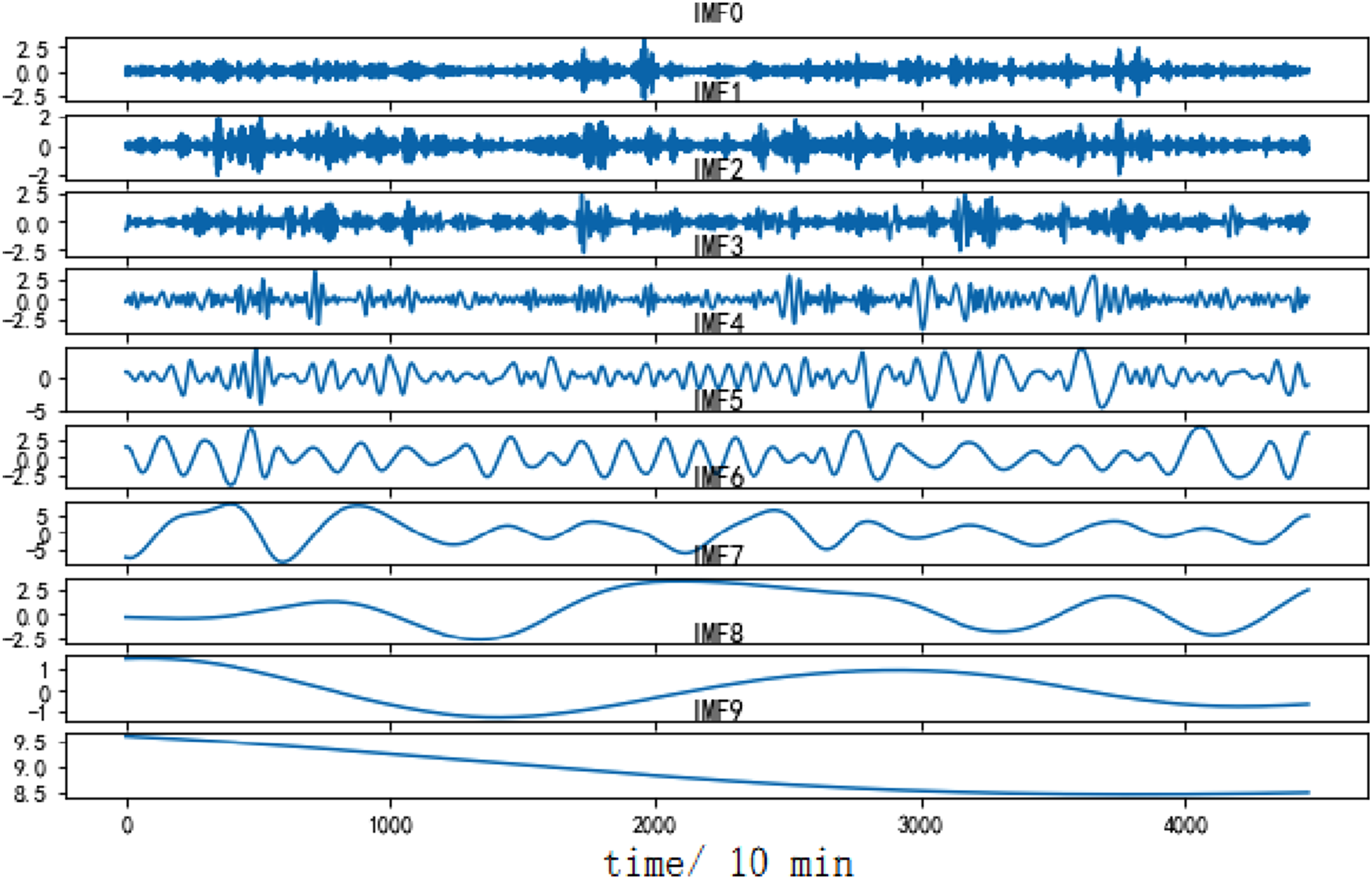
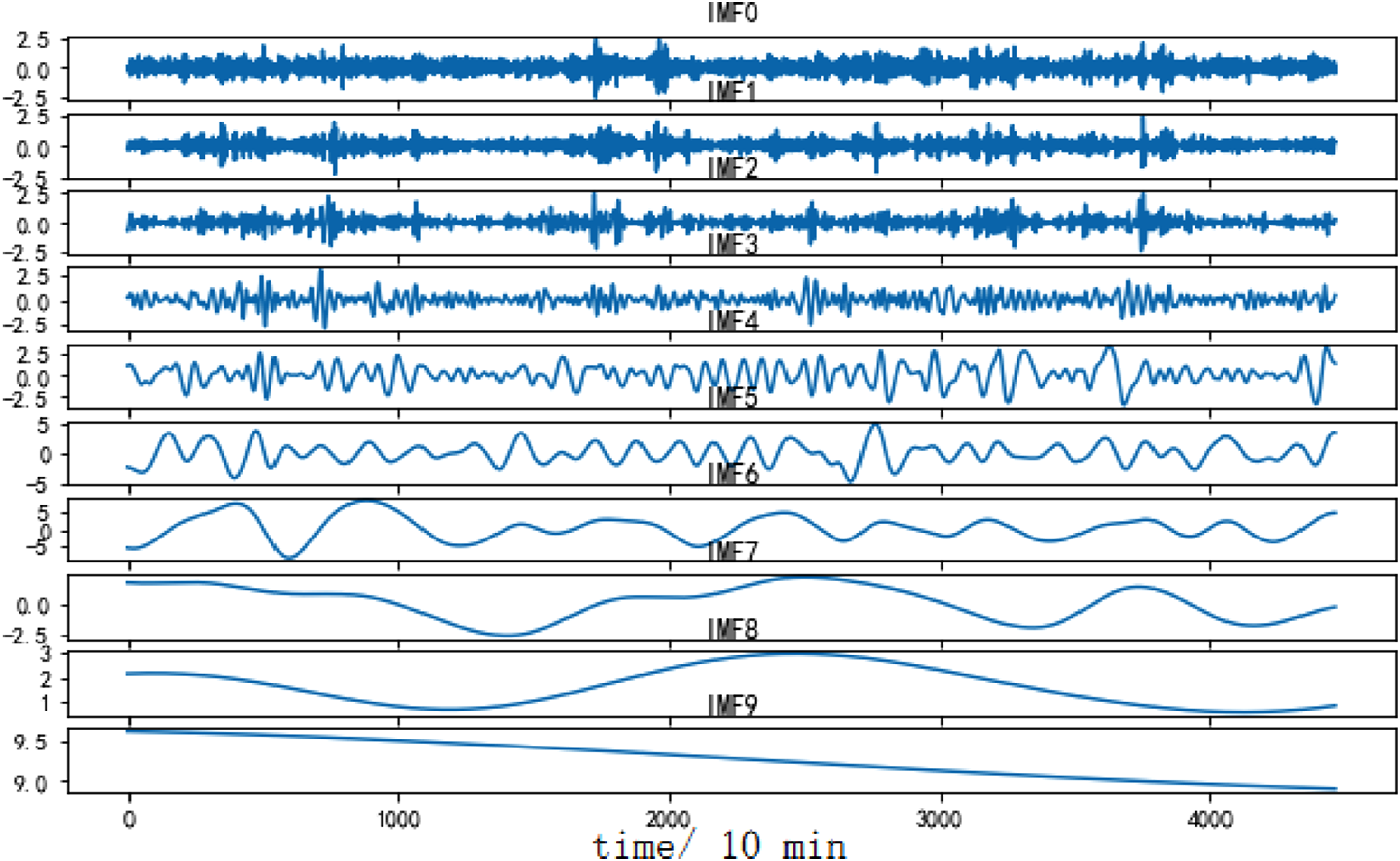
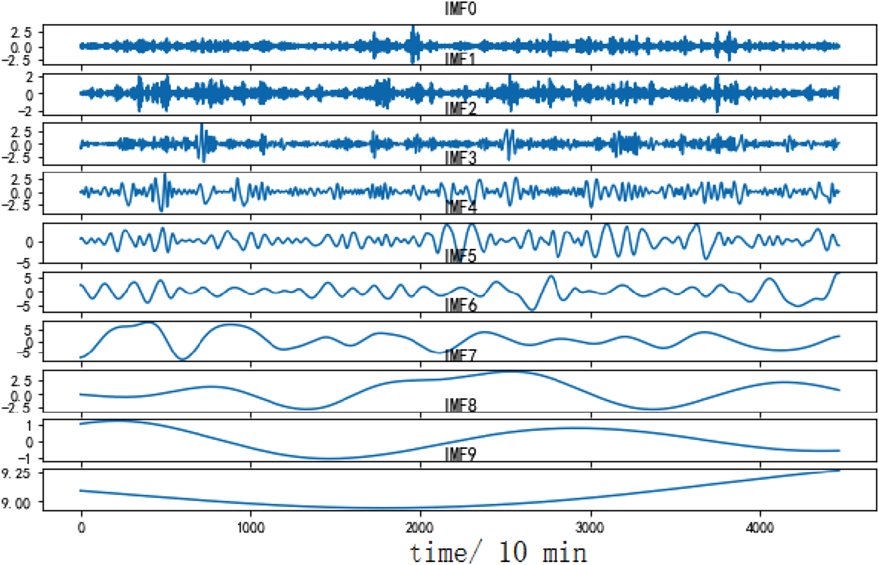
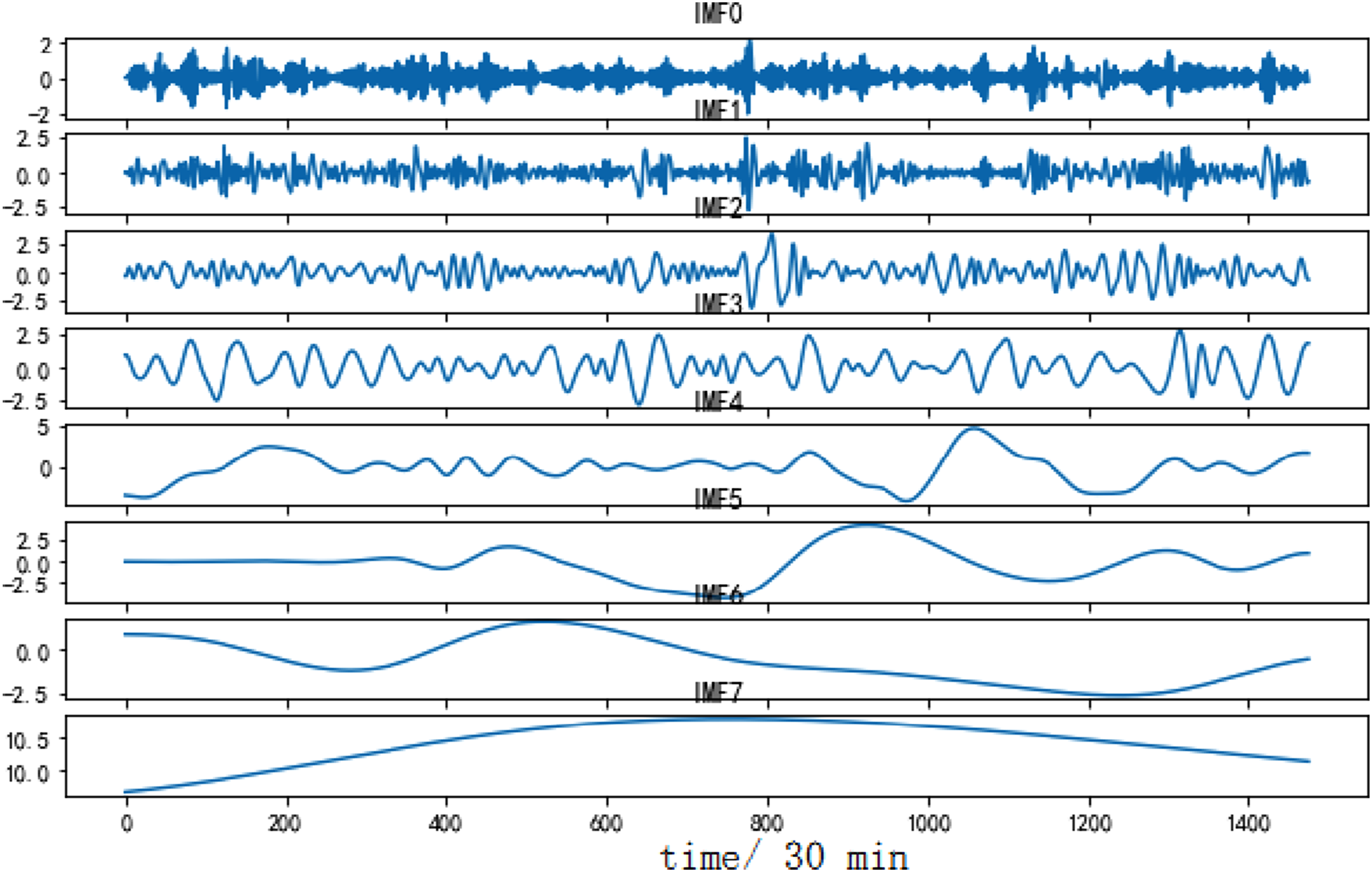
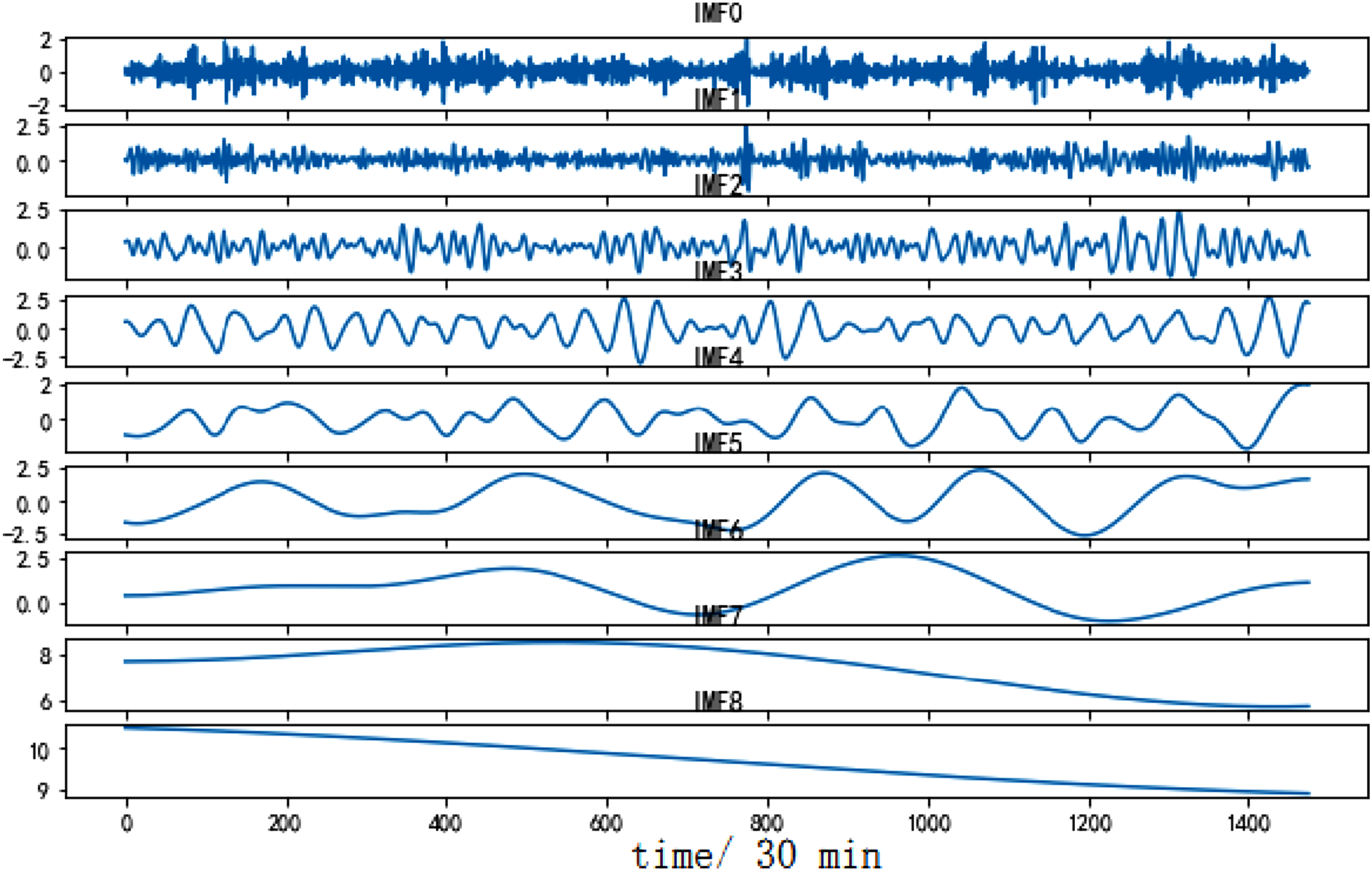
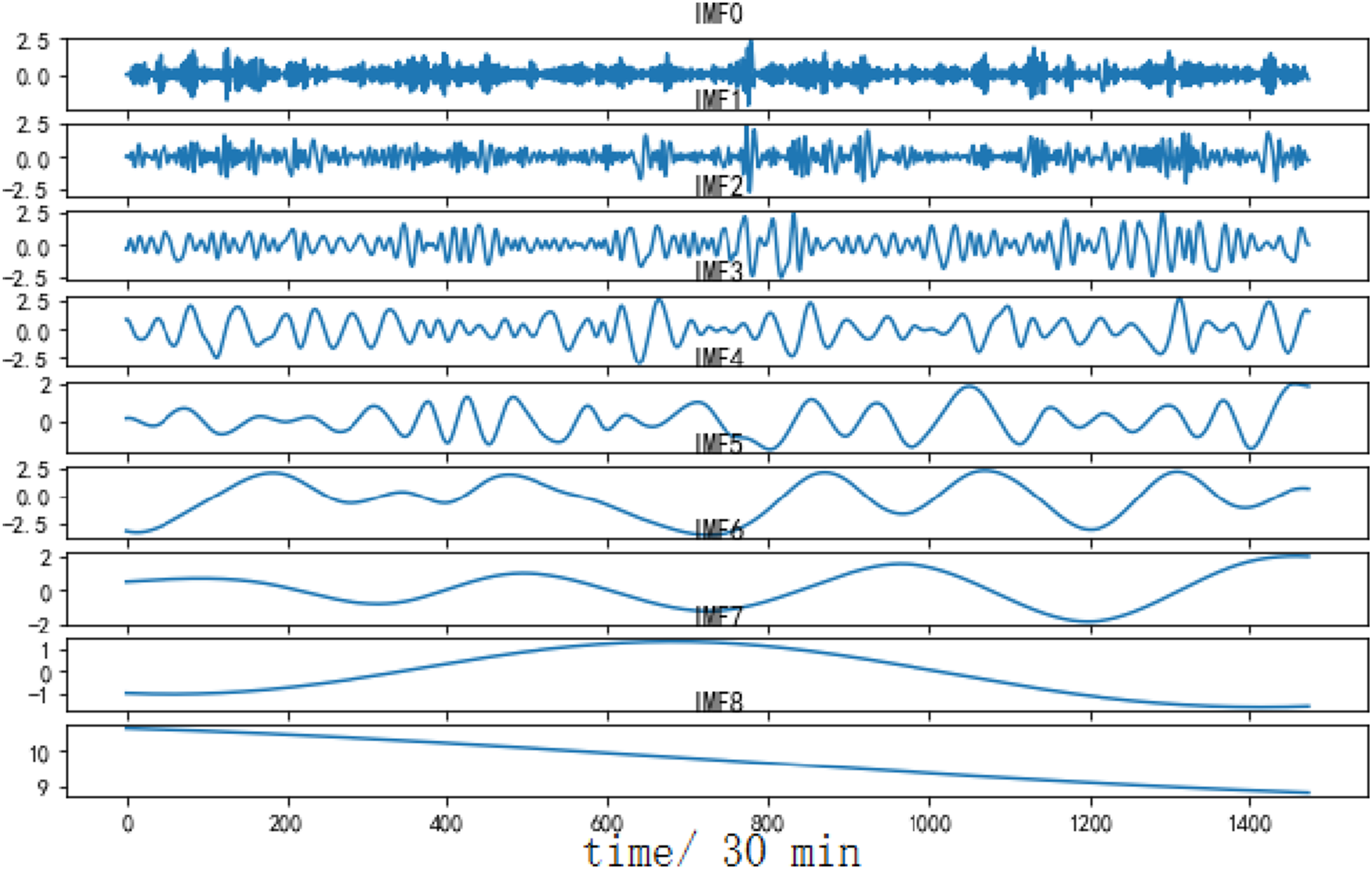
Using the decomposition results of dataset A to analyze, CEEMDAN decomposes the dataset A to generate 9 IMF components and one residual component. Among them, IMF0 to IMF2 belong to high-frequency IMF, with high fluctuation frequency and short wavelength. IMF3 to IMF5 belong to the intermediate frequency IMF, with a decrease in frequency and a corresponding increase in wavelength. IMF6 to IMF8 belong to low-frequency IMFs, with lower frequencies and longer wavelengths. Different IMFs carry different element from the original sample and also have their own fluctuation frequencies. Similarly, for the dataset B, CEEMDAN also achieves the best decomposition effect.
The components obtained from CEEMDAN and EEMD decomposition exhibit overall consistency, both of which can effectively suppress mode aliasing in EMD decomposition and have good decomposition effects. Aiming at compare the effectiveness of the three decomposition algorithms include CEEMDAN, EEMD, and EMD more clearly, the decomposed components are reconstructed and the residual between the reconstructed components and the original dataset is calculated. The specific results are shown in Figures 12 and 13. Comparison of residuals of decomposition reconstruction for dataset A. Comparison of residuals of decomposition reconstruction for dataset B.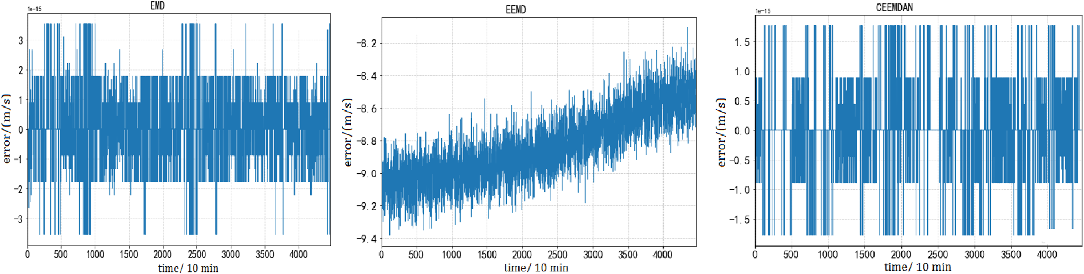
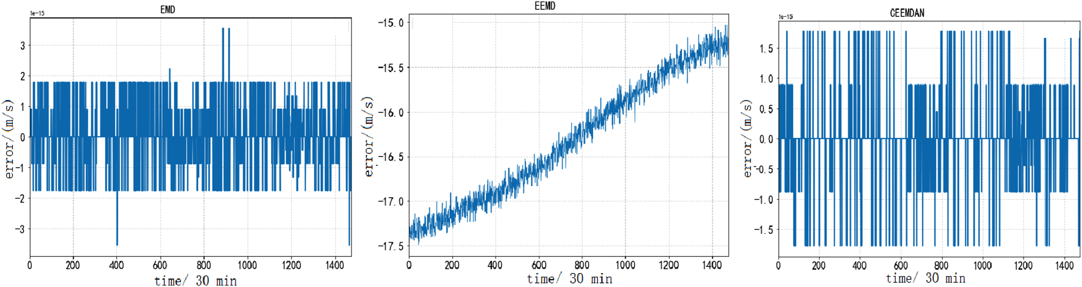
The value of the reconstructed residual is an important indicator for judging the decomposition effect. The smaller the residual, the smaller the difference between the decomposed signal and the original signal, and the better the decomposition effect. From Figures 12 and 13, it can be seen that for dataset A and dataset B, the residual range of CEEMDAN is between −1.5 and 1.5, which is smaller than the residuals of EEMD and EMD algorithms. Therefore, the CEEMDAN algorithm has higher reconstruction ability for short-term wind speed data.
Hyper-parameters optimization results of BiLSTM
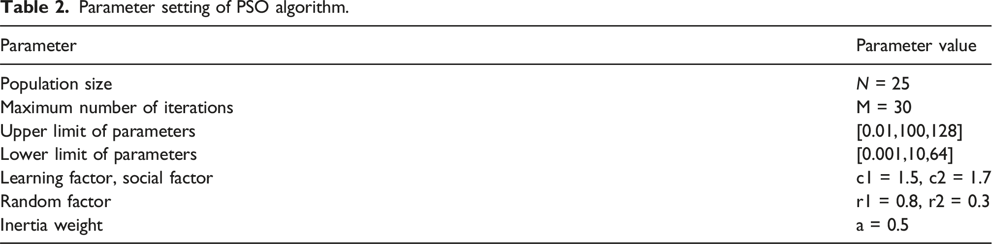
Parameter setting of PSO algorithm.
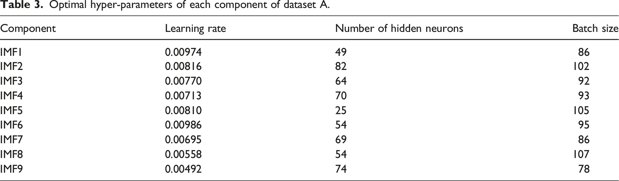
Optimal hyper-parameters of each component of dataset A.
Optimal hyper-parameters of each component of dataset B.

The introduction of attention mechanism can significantly improve the identification ability of BiLSTM model for key local features of input sequence when modeling the components obtained from each decomposition. This mechanism enhances the contribution of important time step features to network parameter optimization by adaptively learning the attention weight distribution of sequence elements, while maintaining the model complexity equivalent to the original structure, thus achieving accurate capture of the dynamic characteristics of the sequence and improving prediction accuracy. Figure 14 shows the distribution of weights for the attention mechanism corresponding to the 10 components of dataset A after CEEMDAN decomposition. Similarly, the distribution of attention mechanism weights corresponding to the nine components of dataset B after CEEMDAN decomposition is shown in Figure 15. The distribution of weights for the attention mechanism corresponding to the 10 components (dataset A). The distribution of weights for the attention mechanism corresponding to the 9 components (dataset B).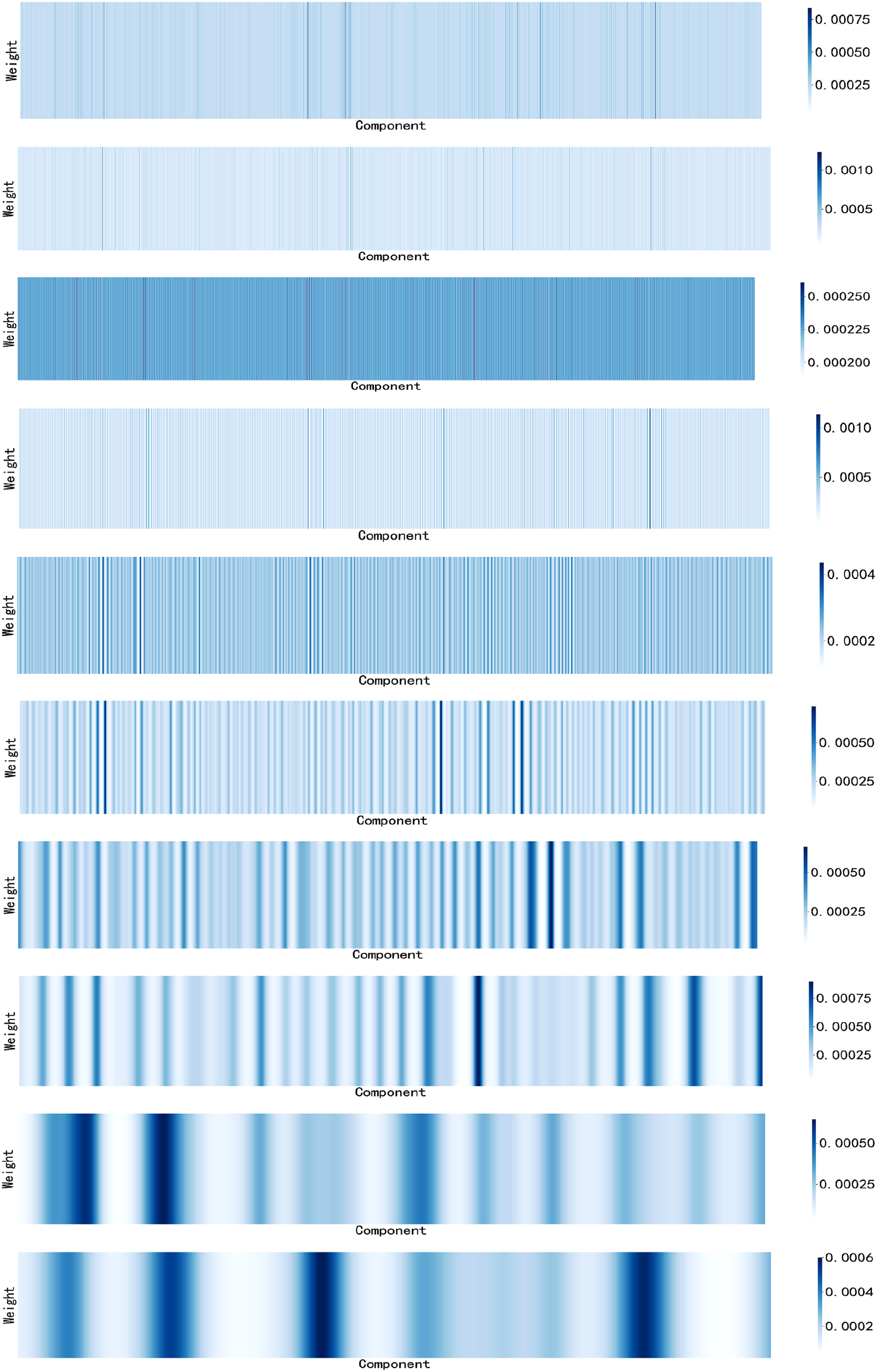

From Figures 14 and 15 above, it can be seen that adding an Attention layer to BiLSTM can calculate the similarity between the current time and historical time, and generate normalized attention weights through the Softmax function. The weight matrix is multiplied with the output of BiLSTM to achieve dynamic weighted fusion of temporal features, highlighting the contribution of key time steps.
Wth the purpose of to verify the prediction result, this paper adopts RMSE, Mean Absolute Error (MAE), Mean Absolute Percentage Error (MAPE) and coefficient of determination (R2) as the evaluation indexes, which are calculated by the following formulas:
RMSE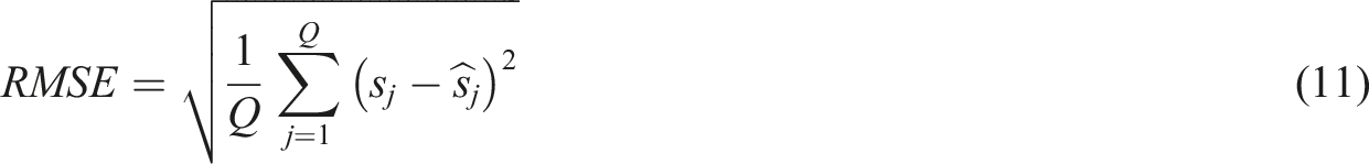
MAE
MAPE
R2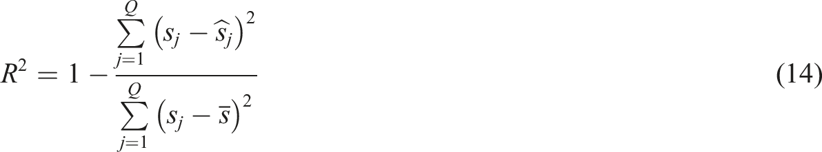
Ablation experiment
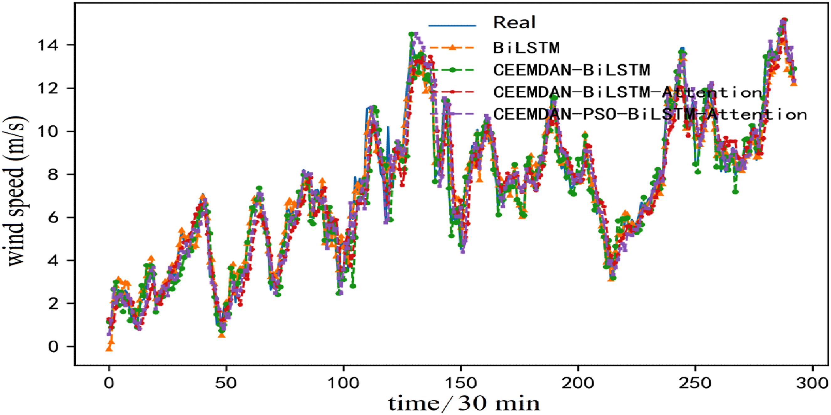
BiLSTM model, CEEMDAN-BiLSTM, BiLSTM-Attention and CEEMDAN-BiLSTM-Attention are chosen to verify the effective of the designed approach. The forecasting results for dataset A and dataset B are provided in Figures 16 and 17, respectively. Among them, the hidden neurons are 32 and the batch size is 64. Comparing the real and forecasted value curves of each model in Figures 16 and 17, we can find the forecasted values of each model are closer to the real values, but the forecasted curve of the designed CEEMDAN-PSO-BiLSTM-Attention has the largest overlap with the actual value curve. Ablation experiment results of dataset A. Ablation experiment results of dataset B.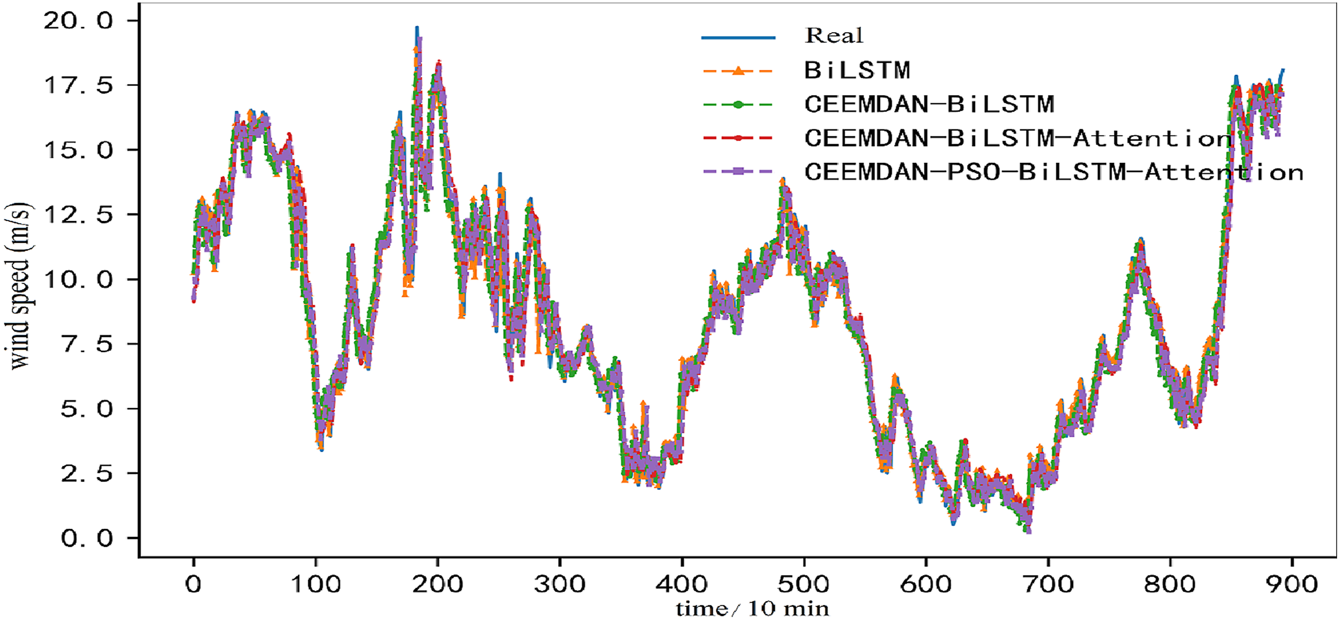
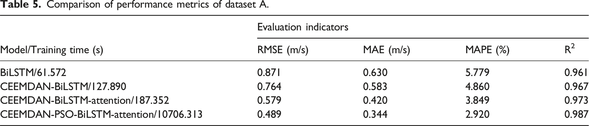
Comparison of performance metrics of dataset A.
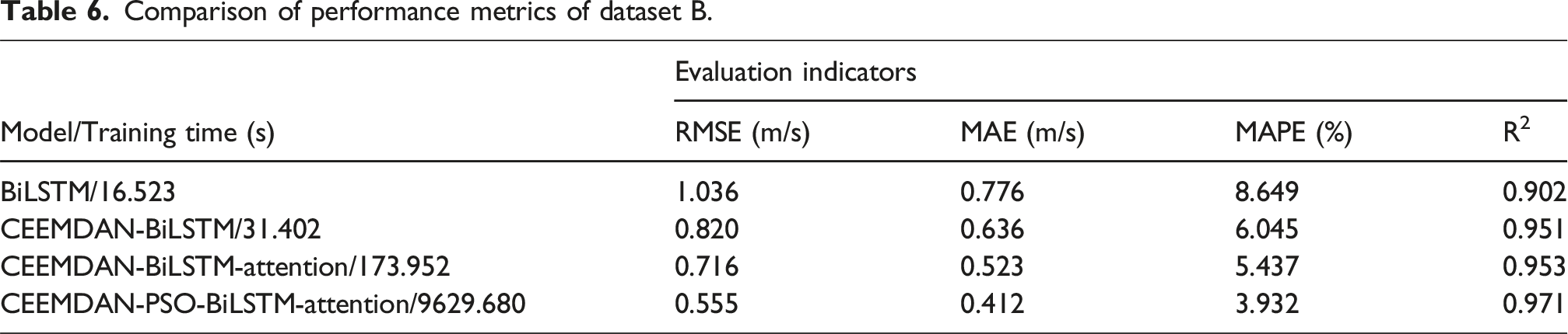
Comparison of performance metrics of dataset B.
Comparison with classical models
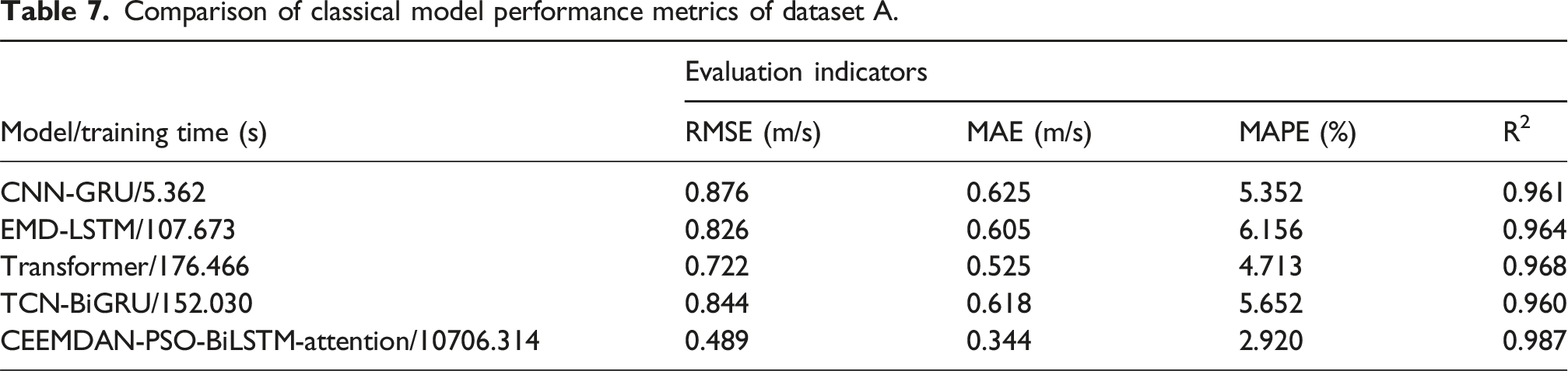
Aiming to further illustrate the superiority of the CEEMDAN-PSO-BiLSTM-Attention, this experiment chooses four classical model include CNN-GRU, EMD-LSTM, Transformer and Temporal Convolutional Network and Bi-directional Gated Recurrent Unit (TCN-BiGRU) for comparison experiments. The number of 1D convolutions of CNN is set to be 64, the size of convolution kernel is 3 × 3, and the number of GRU implied neurons is 32. EMD decomposes the original wind speed data into 8 IMF components and a residual. For Transformer, batch size is 32, n_head is 8, number of epochs is 100, learning rate is 0.0001, drop_out is 0.1 For TCN-BiGRU model, the number of hidden layer neurons is 10, the activation function is ReLU, the number of convolution kernels is 1, the size of convolution kernels is 5, and the learning rate is 0.01. Figures 18 and 19 show the prediction results of these models for two datasets, respectively. From the comparison between the real values and the forecasted values of various models in the two figures, the obvious conclusion is that the CEEMDAN-PSO-BiLSTM-Attention has good fitting and can better track the change of actual short-term wind speed. The prediction results of these models for dataset A. The prediction results of these models for dataset B.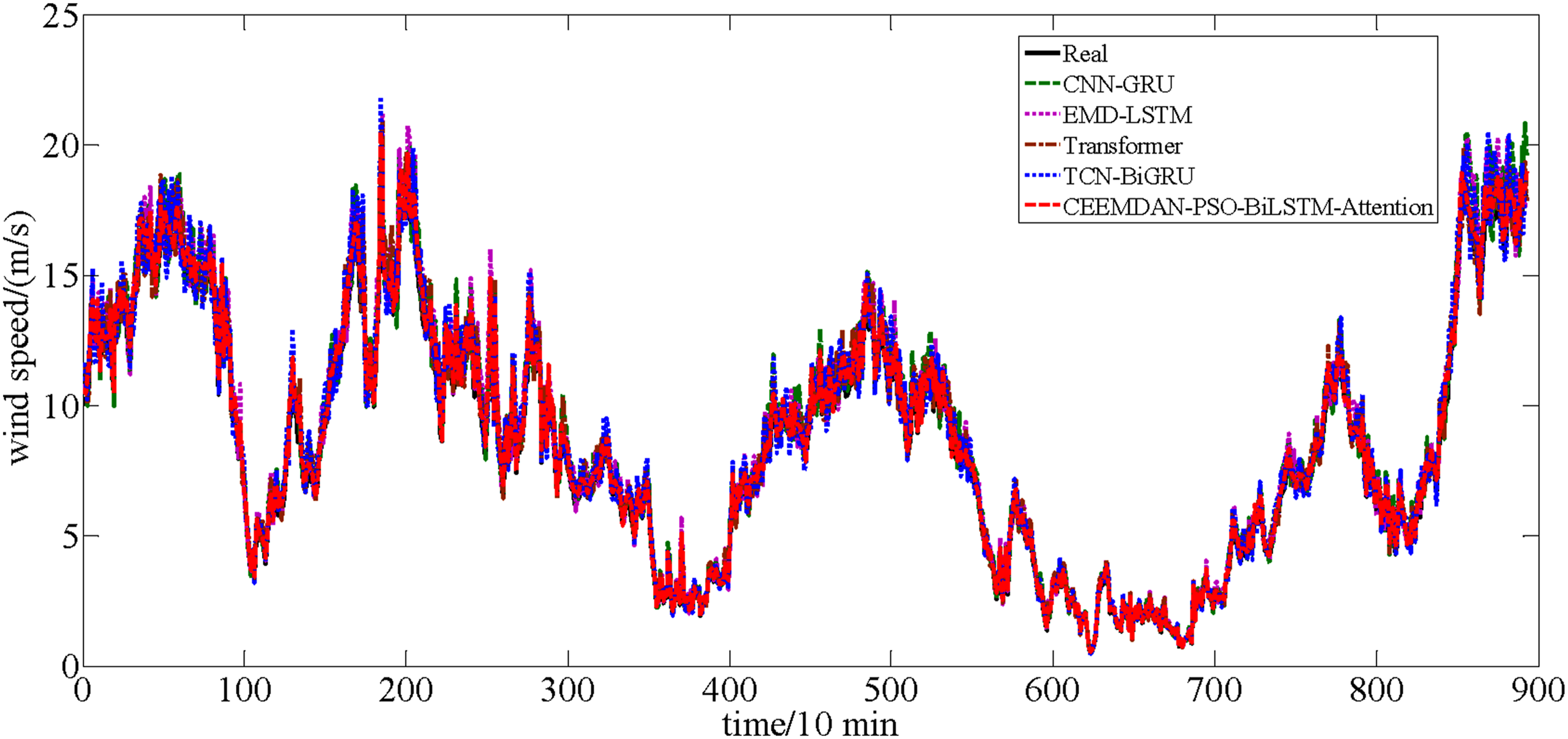
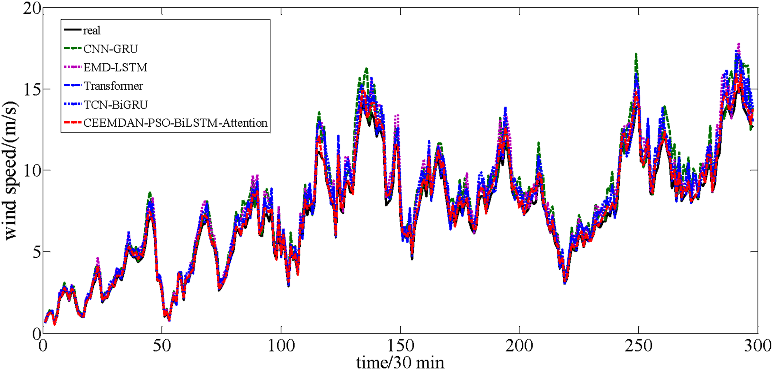
Comparison of classical model performance metrics of dataset A.
Comparison of classical model performance metrics of dataset B.

Due to the CEEDMAN decomposition algorithm generating multiple components, each component requires PSO algorithm for hyper-parameter optimization, resulting in slightly longer training time for the model. Offline training can be used for online applications, combined with timed retraining to alleviate time pressure.
Multi-step prediction results
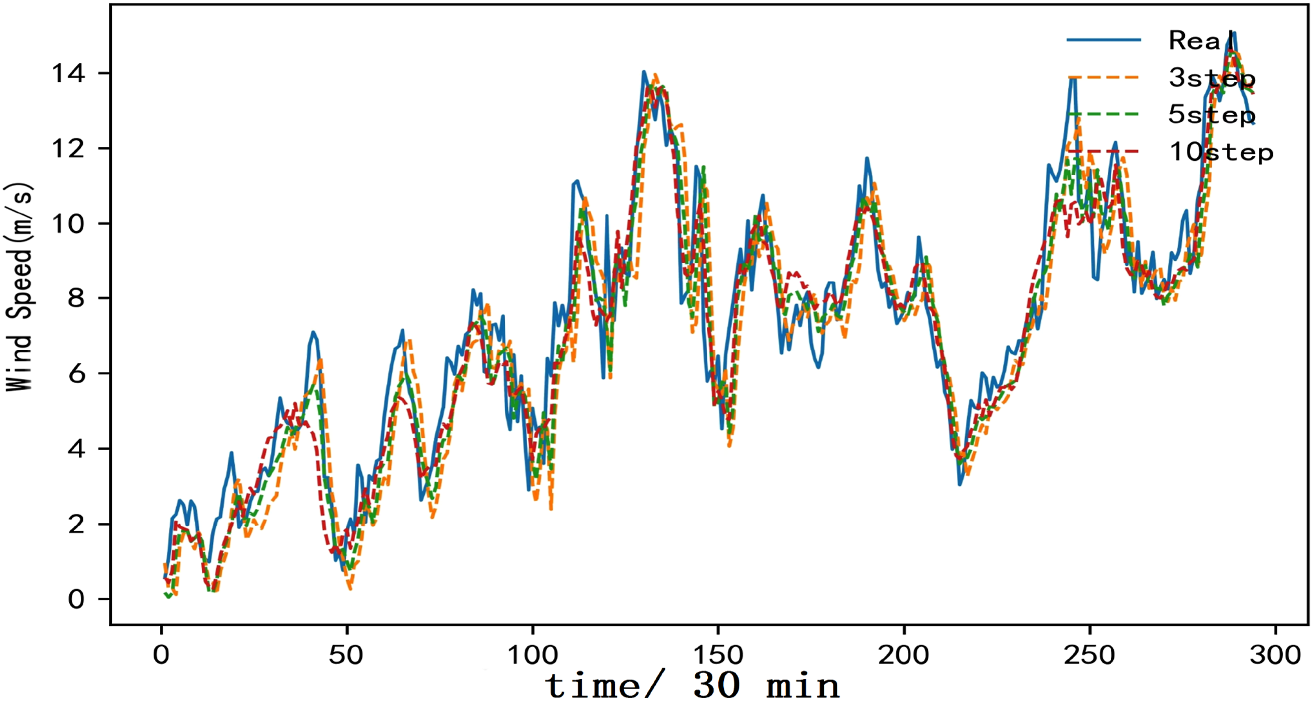
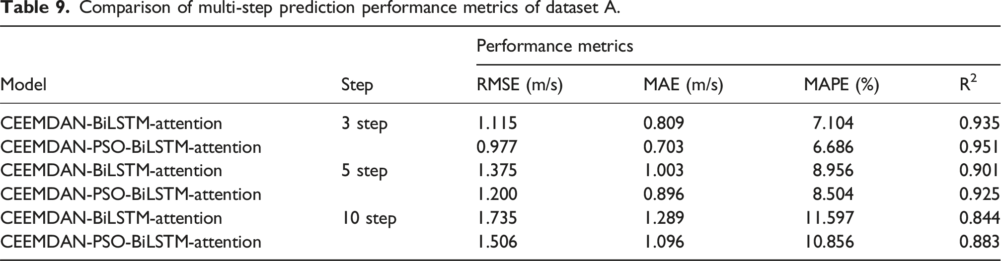
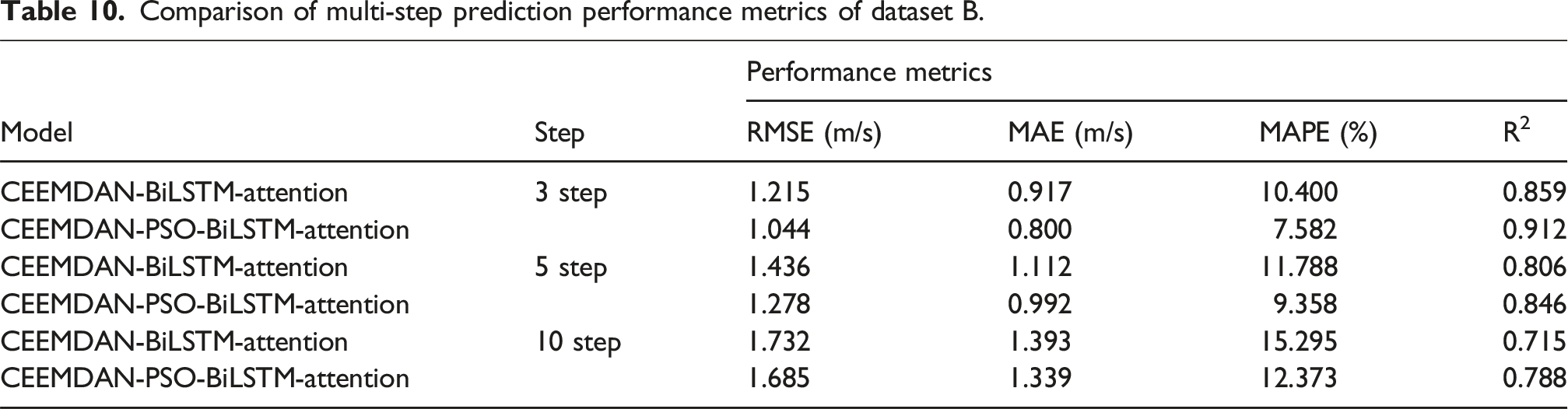
Multi-step prediction is an effective method to test the accuracy of forecasting models (Yu et al., 2025). In many forecasting applications, it is necessary to predict the trend over a future period of time, for example, multi-step wind speed prediction with large step length can provide more abundant time for grid adjustment in wind farms. Therefore, the CEEMDAN-BiLSTM-Attention model and the proposed CEEMDAN-PSO-BiLSTM-Attention are chosen to perform three-step, five-step, and ten-step forecasting experiments, respectively. Figure 20 presents the multi-step forecasting results of dataset A. Figure 21 presents the multi-step forecasting results of dataset B. Multi-step forecasting results (dataset A). Multi-step forecasting results (dataset B).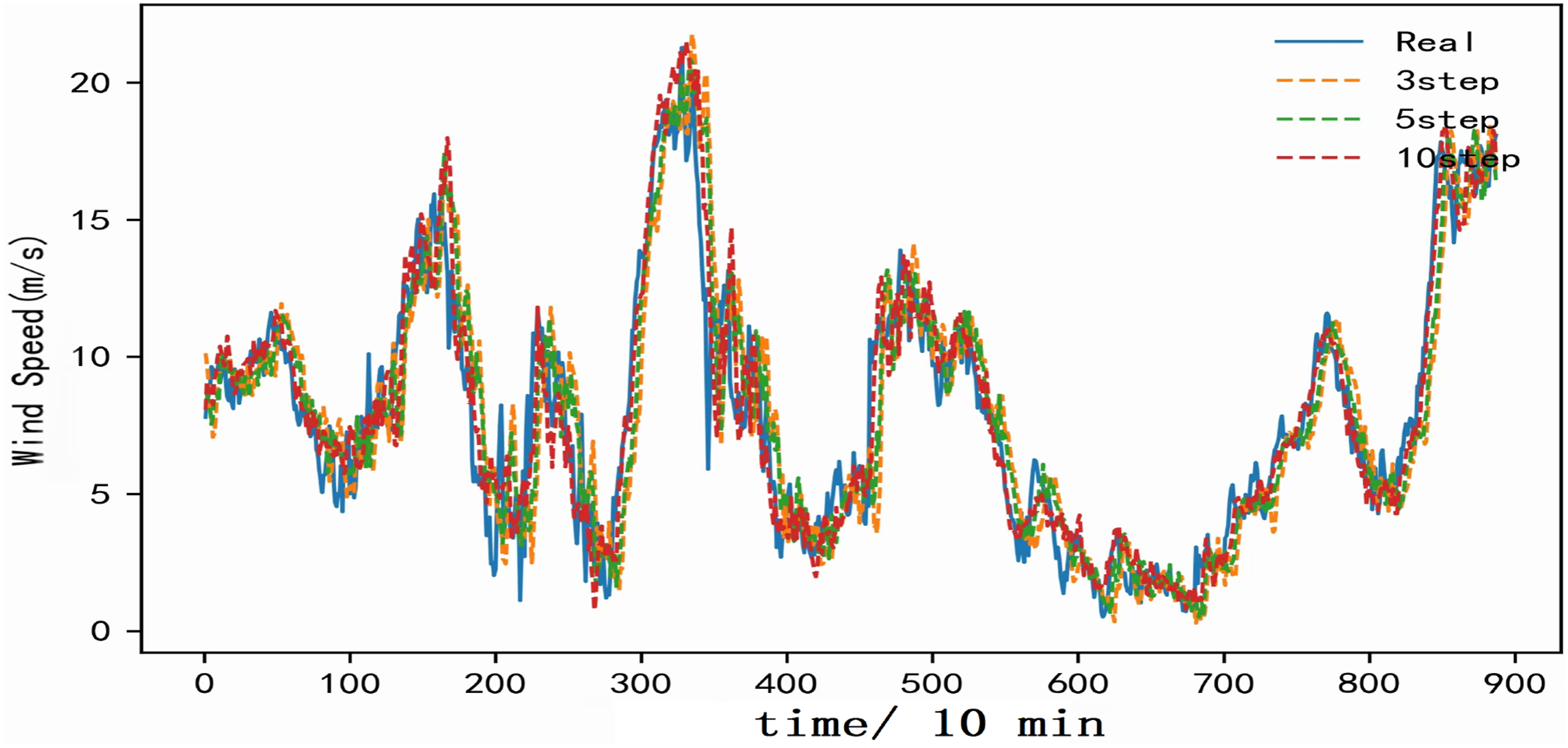
Comparison of multi-step prediction performance metrics of dataset A.
Comparison of multi-step prediction performance metrics of dataset B.
Conclusion
In our paper, the CEEMDAN algorithm is selected to process the fluctuating short-term wind speed data, which is decomposed into smooth and regular signals to decrease the complexity and volatility of the short-term wind speed sample. The decomposed component is then modeled and predicted using BiLSTM-Attention model, which not only captures the long-term dependence on the historical time step in the sequence, but also handles importance-based sampling. Besides, the PSO algorithm is adopted to acquire the optimal key hyper-parameters in BiLSTM, which decreases forecasting error and improves the forecasting effect. Two sets of real short-term wind speed datasets are collected as the study target. Through ablation experiments, comparison with other models, multi-step prediction and other results explain the efficiency of the designed approach.
The proposed model still needs to improve in terms of training time. In the future, some hardware accelerators such as Tensor Processing Unit and Field Programmable Gate Array can be combined to further raise the speed of model training. These accelerators are specifically optimized for machine learning and deep learning tasks, providing higher computational performance and energy efficiency.
Footnotes
Authors contributions
Funding
The authors disclosed receipt of the following financial support for the research, authorship, and/or publication of this article: This paper is supported by the Science Research Project of Liaoning Education Department (LJKZ0143), and the Open Project of State Key Laboratory of Synthetical Automation for Process Industries (2023-kfkt-01).
Declaration of conflicting interests
The authors declared no potential conflicts of interest with respect to the research, authorship, and/or publication of this article.
Data Availability Statement
The data used to support the results of this study can be obtained from the corresponding author.