The January effect,does options trading matter?

Abstract

This study examines the effect of options trading on the January effect in the period 1996–2009. The options market offers investors an alternative trading venue that circumvents several trading limitations in the equity market and hence enables a higher level of arbitrage activities. In a cross-sectional setting, we find that optioned stocks exhibit significantly lower risk-adjusted returns in January than non-optioned stocks. This effect is not attributed to firm size, illiquidity, or transaction costs. We also find that the January effect is not only smaller but also considerably more short-lived for optioned stocks than for non-optioned stocks. In a firm-specific setting, January risk-adjusted returns are found to be significantly lower in the post-options-listing period than in the pre-options-listing period. These findings support the proposition that options trading enhances information-based trading activities and hence improves the informational efficiency of the equity market.

JEL classifications: G10, G11, G12, G14

Keywords

January effect informational efficiency options trading

1. Introduction

The January effect refers to the phenomenon that stock prices, especially those of small market capitalization firms, exhibit a significant surge after the turn of the calendar year. On the one hand, this phenomenon is one of the most intriguing anomalies in the finance literature, given that there is no evidence toward its disappearance, although investors have been aware of this effect for several decades. On the other hand, the January effect may not be a manifestation of market inefficiency, because exploitation of this phenomenon is to a large extent discouraged by high transaction costs and low liquidity for small market capitalization and low-priced stocks.

This study examines the effect of options trading on the magnitude of the January effect in the US markets over the period 1996–2009. The options market offers low-cost, high-leverage transactions, and options trading is not subject to short sales constraints. These desirable qualities of options trading enable several trading strategies that are economically infeasible otherwise and hence facilitate a higher level of information-based trading activities.¹ For example, investors can purchase call options in December to trade the January effect. Since arbitrage aligns options and stock prices, there will also be price pressure on stock prices, and hence the January effect may begin ahead of January and be spread out over a longer period until it eventually fades away. We conjecture that if investors exploit the January effect by trading in the options market, then options trading portends a reduced magnitude for the January effect.

We document three important effects of options trading on the January effect in this study. First, in a cross-sectional setting, we find compelling evidence that optioned stocks exhibit significantly lower risk-adjusted returns in January than non-optioned stocks. This finding holds when we include factors that control for firm size, transaction costs, illiquidity, and other factors that may also provide plausible explanations for the January effect. The negative relation between options trading and risk-adjusted returns is almost exclusive to January, since such a relation is generally not found in other months. Second, we find that the January effect is not only reduced but also considerably more short-lived for optioned stocks than for non-optioned stocks. For example, in the smallest size group, the stock prices of non-optioned stocks drift upward in the first 33 trading days of the year, while the stock prices of optioned stocks drift up only in the first 8 trading days of the year. Finally, in a firm-specific approach, we compare January risk-adjusted returns in the periods before and after an options listing for a sample of firms that were optioned during the period 1998–2007. The average risk-adjusted return in January is found to be significantly lower in the post-options-listing period than in the pre-options-listing period. The alleviation of the January effect due to an options listing is most pronounced for small stocks, illiquid stocks, and low-priced stocks. To aid the firm-specific analysis, we also examine the January return in the re- and post-options listing periods for matched samples of non-optioned stocks. We employ three matched samples: (i) matched sample by pre-options-listing January return and firm size, (ii) matched sample by pre-options-listing January return and volatility, and (iii) matched sample by the propensity score of having an options listing. Across three different matched samples, we find that matched non-optioned stocks exhibit no significant change in January risk-adjusted return between the pre- and post-options-listing periods of optioned stocks.

Findings in our study point toward the proposition that options trading generally mitigates the January anomaly. The mitigation is most effective among stocks whose transaction costs and illiquidity are likely to deter arbitrage activities in the equity market. This is in line with the contention that options are superior investment vehicles that help investors overcome several trading limitations in stocks and their use improves the efficiency of pricing in the equity market. This study therefore adds to an emerging literature that suggests that options are not simple redundant securities but, in fact, offer a preferred venue for information-based trading activities.

The remainder of this paper is organized as follows. Section 2 briefly reviews the related literature and this study’s motivations. Section 3 discusses the data and sample properties. Section 4 presents the main empirical findings. Finally, Section 5 concludes the study.

2. Related literature

The January or “turn-of-the-year” effect refers to the well-documented phenomenon that stock returns are significantly higher in January than in other months. Wachtel (1942) first reported evidence of seasonality in the Dow Jones Industrial Average and found that the index exhibited significant positive returns and bullish signals in January during the period 1927–1942. More than three decades later, Rozeff and Kinney (1976) brought the phenomenon to the attention of both academics and practitioners. They demonstrated that the average return of the equal-weighted NYSE index was more than eight times higher in January than in other months over the period 1904–1974. Increased interests in the existence of this empirical regularity led to several follow-up studies employing different sample periods, larger data sets, and more advanced empirical analyses. These studies generally agreed that the January effect poses a serious challenge to the hypothesis that the market is informationally efficient (Bhardwaj and Brooks, 1992; Haugen and Jorion, 1996; Haugen and Lakonishok, 1988; Keim, 1983; Reinganum, 1983).²

The January effect is found to be most pronounced among small market capitalization stocks, illiquid stocks, low-priced stocks, and neglected stocks (Bhardwaj and Brooks, 1992; Blume and Stambaugh, 1983; Keim, 1983). The extant literature offers two major possible explanations for the existence of the phenomenon: (1) tax-loss selling, whereby investors sell stocks that have generated losses to claim deductions on taxes and use the tax-loss sale funds together with other funds (Christmas, year-end bonuses and other cash resources) to buy stocks in early January (Branch, 1977; Dyl, 1977; Dyl and Maberly, 1992; Givoly and Ovadia, 1983; Koogler and Maberly, 1994; Reinganum, 1983; Ritter, 1988; Sias and Starks, 1997; Tinic et al., 1987), and (2) window dressing, whereby professional portfolio managers buy stocks with positive prior returns and sell stocks with negative prior returns to reveal more respectable year-end portfolio holdings to clients (Athanassakos, 1992; Griffiths and White, 1993; Haugen and Lakonishok, 1988; He et al., 2004; Lakonishok et al., 1991).

Although investors have been aware of the phenomenon for several decades and there have been numerous studies, it is intriguing that the January effect shows no sign of weakening or disappearing over time (Haug and Hirschey, 2006). The highlighted impediments to exploiting the January effect are high transaction costs and the illiquidity of small capitalization and low-priced stocks. For example, Stoll and Whaley (1983) show that the two-way transaction cost for small stocks can be as high as 5%, which would eat up most of the profits from a strategy that quickly buys and sells these stocks at the turn of the year.³ Liu (2006) documents a significant liquidity premium in January and argues that this is an important priced risk factor. The limits to arbitrage or risks imply that the phenomenon of high stock returns in January may not necessarily refute the efficient market hypothesis.

The options market can offer a medium for investors to circumvent several frictions in the equity market and exploit the January effect. Several studies propose that options are superior investment vehicles because they enable low-cost, high-leverage transactions, and options trading is not subject to short-sale constraints (Back, 1993; Biais and Hillion, 1994; Black, 1975; Manaster and Rendleman, 1982).⁴ Black (1975) states

Since an investor can get more action for a given investment in options than he can by investing directly in the underlying stock, he may choose to deal in options when he feels he has an especially important piece of information.⁵

The advantages that options trading offers would allow investors to trade the January phenomenon, whereas trading in the equity market may be significantly more costly or even economically infeasible. For example, instead of purchasing 10,000 shares at $5 each at the turn of the year, an investor can buy 100 call options at a premium of $0.50 – a cost that is therefore a fraction of the capital required in the equity market. Also, investors can preempt the tax-loss selling of a stock in December by going long in put options, while short selling in the equity market would be much more difficult. We propose that if options traders employ options to exploit the January phenomenon, the magnitude of the effect will diminish or utterly disappear for the stocks for which options trading is readily available.⁶

3. Data and sample

This study’s sample comprises of firms traded on the NYSE/AMEX and NASDAQ for the period 1996–2009. We identify stocks with available options trading and the first day of options trading from OptionMetrics. Stock return, stock price, and Fama and French factors are from CRSP. Book-to-market ratios are from Compustat and the number of analysts following each stock is culled from IBES. For the period 1996–2004, we obtain the probability of information-based trading (PIN) dataset, as in Easley et al. (2002).⁷

Table 1 presents descriptive statistics on the characteristics of stocks in the sample over the period 1996–2009. Here, BETA is the beta of the portfolio to which the stock belongs. We first estimate pre-ranking betas for individual stocks using monthly returns from two to five years. We then sort the stocks into 50 portfolios in every January based on these pre-ranking portfolio betas and compute the equal-weighted returns for all portfolios. Finally, we estimate the post-ranking portfolio betas for these 50 portfolios using the full sample period. Here, SIZE is the natural logarithm of market capitalization at the end of year t – 1 and BM is the natural logarithm of the ratio of the book value of common equity to market capitalization at the end of year t – 1. We follow Amihud (2002) to compute the illiquidity measure (ILLIQ) as the ratio of daily absolute stock returns to dollar trading volume in year t – 1. The mean and median stock prices are 27.12 and 18.92, respectively. The mean and median number of analysts following each stock are 4.79 and 3.78, respectively. Here, TOV is the natural logarithm of the average monthly turnover in year t − 1, MOM is the stock return in the prior 12 months leading up to year t, and IDIOVOL is idiosyncratic volatility measured as the variance of the residuals from the Fama and French (1992) three-factor model estimated in the five-year period leading up to year t. The mean and median of the PIN are 0.22 and 0.19, respectively, and OPT is a dummy variable taking the value of one for optioned stocks, and zero otherwise. Around 46% of stocks in the sample have options trading. Panel B of Table 1 presents the percentage of optioned stocks in each quintile of firm SIZE, ILLIQ, and PRICE. Table 2 presents the correlations among variables. Panel A presents the correlation matrix for non-optioned stocks and Panel B presents the correlation matrix for optioned stocks.

Table 1.

Descriptive statistics, 1996–2009.

Panel A: Summary statistics
	Mean	Median	Q1	Q3
BETA	1.05	0.97	0.64	1.49
SIZE	5.83	5.76	2.34	8.89
BM	−0.57	−0.48	−2.32	0.79
ILLIQ	1.28×10^–5	0.07×10^–5	0.02×10^–5	17.8×10^–5
PRICE	27.12	18.92	5.00	60.25
NANA	4.79	3.78	2.00	5.00
TOV	−3.12	−3.02	−6.36	−4.65
MOM	11.82	8.09	−21.21	27.32
IDIOVOL	3.56×10^–2	2.19×10^–2	1.52×10^–2	3.87×10^–2
PIN	0.22	0.19	0.14	0.34
OPT	0.46	0	0	1

Panel B: Distribution of optioned stocks by quintiles of firm characteristics
	SIZE Quintile	ILLIQ Quintile	PRICE Quintile

Q1	11.37%	7.66%	8.08%
Q2	24.96%	20.01%	29.75%
Q3	43.67%	43.62%	41.38%
Q4	68.60%	65.19%	50.94%
Q5	84.37%	76.61%	74.41%

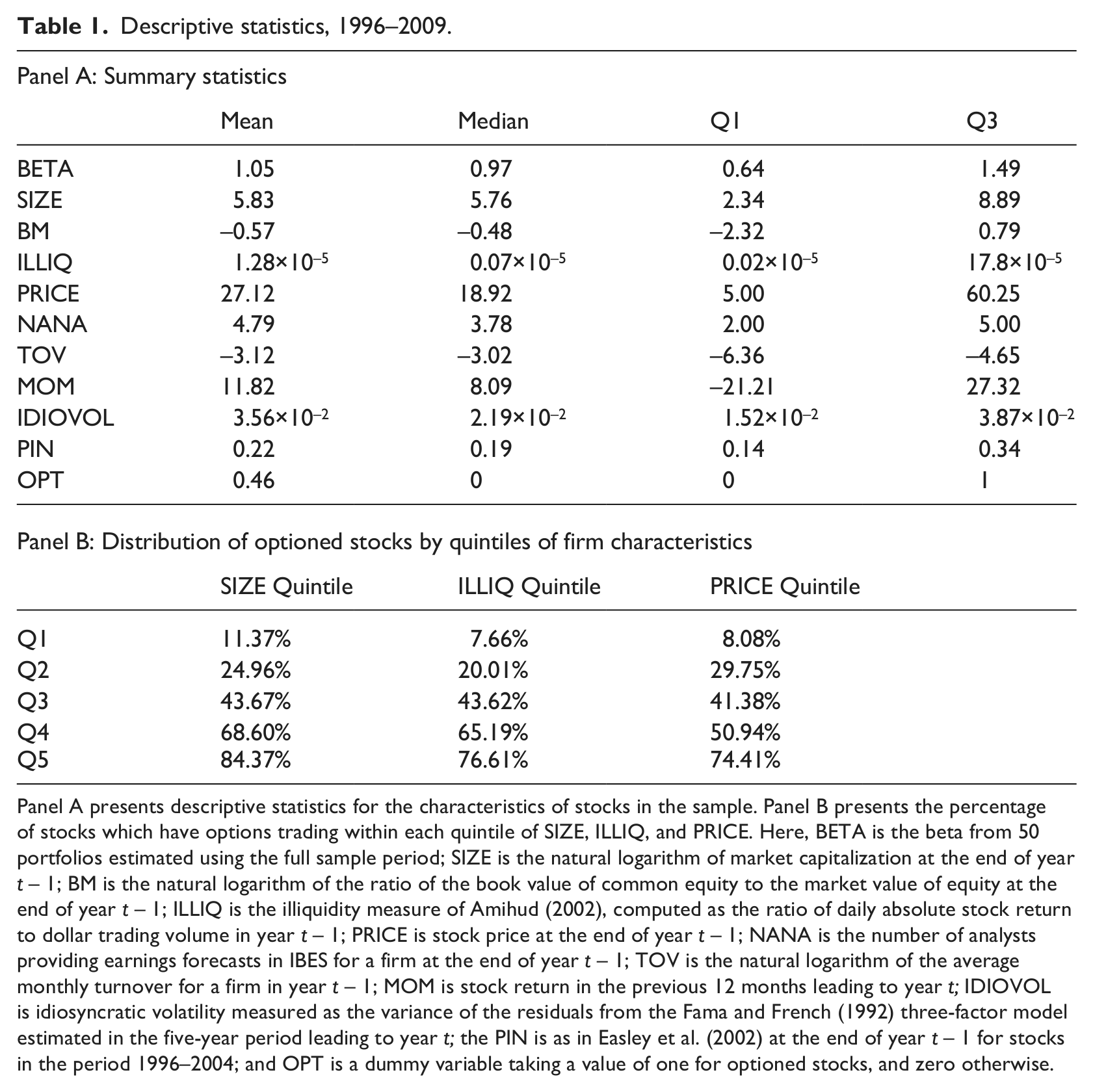
Panel A presents descriptive statistics for the characteristics of stocks in the sample. Panel B presents the percentage of stocks which have options trading within each quintile of SIZE, ILLIQ, and PRICE. Here, BETA is the beta from 50 portfolios estimated using the full sample period; SIZE is the natural logarithm of market capitalization at the end of year t – 1; BM is the natural logarithm of the ratio of the book value of common equity to the market value of equity at the end of year t – 1; ILLIQ is the illiquidity measure of Amihud (2002), computed as the ratio of daily absolute stock return to dollar trading volume in year t – 1; PRICE is stock price at the end of year t – 1; NANA is the number of analysts providing earnings forecasts in IBES for a firm at the end of year t – 1; TOV is the natural logarithm of the average monthly turnover for a firm in year t – 1; MOM is stock return in the previous 12 months leading to year t; IDIOVOL is idiosyncratic volatility measured as the variance of the residuals from the Fama and French (1992) three-factor model estimated in the five-year period leading to year t; the PIN is as in Easley et al. (2002) at the end of year t – 1 for stocks in the period 1996–2004; and OPT is a dummy variable taking a value of one for optioned stocks, and zero otherwise.

Table 2.

Correlation matrix.

Panel A: Correlation matrix for non-optioned stocks
	SIZE	BM	ILLIQ	PRICE	NANA	TOV	MOM	IDIOVOL	PIN
BETA	−0.16	−0.10	0.04	−0.14	−0.03	0.22	−0.13	0.36	0.16
SIZE		−0.23	−0.33	0.41	0.25	0.28	0.18	−0.51	−0.50
BM			0.16	−0.19	−0.17	−0.27	−0.01	−0.17	0.13
ILLIQ				−0.21	0.25	−0.46	−0.08	0.29	0.30
PRICE					0.13	0.12	0.16	−0.46	−0.35
NANA						0.14	0.05	−0.25	−0.18
TOV							0.06	0.13	−0.56
MOM								0.10	0.28
IDIOVOL									0.48

Panel B: Correlation matrix for optioned stocks
	SIZE	BM	ILLIQ	PRICE	NANA	TOV	MOM	IDIOVOL	PIN

BETA	−0.10	−0.08	0.03	−0.11	0.06	0.12	−0.03	0.20	−0.10
SIZE		−0.20	−0.29	0.38	0.16	0.21	0.02	−0.33	−0.27
BM			0.02	−0.14	−0.07	−0.17	−0.04	0.02	0.05
ILLIQ				−0.11	0.15	−0.22	0.01	0.14	0.17
PRICE					0.15	0.07	0.03	−0.15	−0.15
NANA						0.02	−0.05	−0.08	−0.02
TOV							−0.04	0.08	−0.28
MOM								−0.14	0.11
IDIOVOL									0.09

This table presents correlations among the characteristics of non-optioned stocks in Panel A and of optioned stocks in Panel B. Here, BETA is the beta from 50 portfolios estimated using the full sample period; SIZE is the natural logarithm of market capitalization at the end of year t – 1; BM is the natural logarithm of the ratio of the book value of common equity to the market value of equity at the end of year t – 1; ILLIQ is the illiquidity measure of Amihud (2002), computed as the ratio of daily absolute stock return to dollar trading volume in year t – 1; PRICE is stock price at the end of year t – 1; NANA is the number of analysts providing earnings forecasts in IBES for a firm at the end of year t – 1; TOV is the natural logarithm of the average monthly turnover for a firm in year t – 1; MOM is stock return in the previous 12 months leading to year t; IDIOVOL is idiosyncratic volatility measured as the variance of the residuals from the Fama and French (1992) three-factor model estimated in the five-year period leading to year t; the PIN is as in Easley et al. (2002) at the end of year t – 1 for stocks in the period 1996–2004.

4. Main empirical findings

4.1. Portfolio January returns between optioned and non-optioned stocks

We begin by showing the portfolio returns of optioned and non-optioned stocks. Table 3 presents the monthly risk-adjusted returns in January and other months for optioned and non-optioned stocks based on firm size, illiquidity, and stock price. We use Fama and French’s (1992) three factors to adjust for risk. We first stratify the sample by quintiles of SIZE, ILLIQ, and PRICE, which are measured at the end of year t – 1. Within each quintile, we compute the average monthly risk-adjusted returns for optioned and non-optioned stocks. This approach controls for the varying degrees of January returns due to firm size, illiquidity, and stock price.

Table 3.

Risk-adjusted returns of non-optioned stocks and optioned stocks, 1996–2009.

Panel A: Risk-adjusted returns of non-optioned stocks and optioned stocks by SIZE quintiles
	Non-optioned stocks	Optioned stocks	Difference
All Months
Q1 (Low)	0.16	−0.07	−0.23**
Q2	0.26	0.06	−0.20**
Q3	0.12	−0.02	−0.14
Q4	0.13	0.05	−0.07
Q5 (High)	0.09	0.04	−0.05
January
Q1 (Low)	7.23	2.54	−4.69***
Q2	4.72	2.81	−1.91***
Q3	2.04	0.77	−1.27***
Q4	1.17	0.11	−1.06***
Q5 (High)	0.60	0.13	−0.47**
Non–January
Q1 (Low)	−0.48	−0.31	0.17*
Q2	−0.15	−0.19	−0.04
Q3	−0.05	−0.09	−0.04
Q4	0.03	0.04	0.01
Q5 (High)	0.04	0.03	−0.01

Panel B: Risk-adjusted returns of non-optioned stocks and optioned stocks by ILLIQ quintiles
	Non-optioned stocks	Optioned stocks	Difference

All Months
Q1 (Illiquid)	0.32	0.05	−0.27*
Q2	0.12	0.03	−0.09
Q3	0.02	−0.05	−0.07
Q4	−0.01	−0.03	−0.02
Q5 (Liquid)	0.04	0.02	−0.02
January
Q1 (Illiquid)	6.63	2.14	−4.49***
Q2	3.67	1.62	−2.05***
Q3	1.06	0.32	−0.74**
Q4	0.67	0.08	−0.59**
Q5 (Liquid)	0.32	0.06	−0.26**
Non–January
Q1 (Illiquid)	−0.25	−0.14	0.11*
Q2	−0.20	−0.11	0.09
Q3	−0.08	−0.08	0.00
Q4	−0.07	−0.04	0.03
Q5 (Liquid)	0.01	0.02	0.01

Panel C: Risk-adjusted returns of non-optioned stocks and optioned stocks by PRICE quintiles
	Non-optioned stocks	Optioned stocks	Difference

All Months
Q1 (Low)	0.44	0.04	−0.40**
Panel C: Risk-adjusted returns of non-optioned stocks and optioned stocks by PRICE quintiles
	Non-optioned stocks	Optioned stocks	Difference
Q2	0.18	0.02	−0.16*
Q3	0.00	−0.06	−0.06
Q4	0.02	−0.03	−0.04
Q5 (High)	0.06	0.06	0.00
January
Q1 (Low)	7.78	2.46	−5.32***
Q2	4.52	1.92	−2.60***
Q3	1.11	0.26	−0.85***
Q4	0.87	0.13	−0.74**
Q5 (High)	0.41	0.10	−0.31**
Non–January
Q1 (Low)	−0.23	−0.18	0.05
Q2	−0.21	−0.15	0.06
Q3	−0.10	−0.09	0.01
Q4	−0.06	−0.04	0.02
Q5 (High)	0.03	0.06	0.03

This table presents monthly risk-adjusted returns for portfolios of optioned and non-optioned stocks sorted by firm size (SIZE), illiquidity (ILLIQ), and stock price (PRICE). The Fama and French (1992) three-factor model is used to adjust for risk. Here ILLIQ is the illiquidity measure of Amihud (2002), computed as the ratio of daily absolute stock return to dollar trading volume in year t – 1, PRICE is stock price at the end of year t – 1, and SIZE, ILLIQ, and PRICE are sorted into quintiles every year. ***, **, and * indicate significance at the 1%, 5%, and 10% level, respectively.

Panel A of Table 3 shows that risk-adjusted returns are generally smaller for optioned than for non-optioned stocks if we consider all months. However, when we separate January from the other months, we find that optioned stocks exhibit significantly lower risk-adjusted returns in January, but the differences in returns between optioned and non-optioned stocks are rather small in the other months. We confirm the January effect, where risk-adjusted return is significantly higher in January and the level of risk-adjusted return monotonically decreases in firm size. For non-optioned stocks, risk-adjusted return is 7.23% for the lowest SIZE quintile and 0.60% for the highest SIZE quintile. We also observe a January effect for optioned stocks, but the risk-adjusted return is of a much lower magnitude. Optioned stocks in the lowest SIZE quintile post 2.54% in January, which is 4.69% lower than that of non-optioned stocks in the same size quintile. We consistently observe lower January risk-adjusted returns for optioned stocks across all SIZE quintiles.

The lower January risk-adjusted returns for optioned stocks after controlling for SIZE quintiles support the proposition that options trading allows investors to exploit the January effect and hence the effect is weakened when options trading is readily available. We continue to examine the implications of options trading for the January effect when controlling for illiquidity and transaction costs.

Panels B and C of Table 3 present the same analysis by stratifying the sample based on Amihud’s (2002) illiquidity measure and stock price. We aim to control for the well-known relations between illiquidity, transaction costs, and the January effect.⁸ Panel B of Table 3 shows that the January risk-adjusted return is monotonically increasing in illiquidity, which indicates that the January effect is also an illiquid stock phenomenon. Within each quintile of illiquidity, optioned stocks exhibit lower January risk-adjusted returns than non-optioned stocks. In the quintile of highest illiquidity, where the January effect is most palpable, risk-adjusted return is 4.49% lower for optioned than for non-optioned stocks. In Panel C of Table 3, the control for stock price also shows the same pattern, that optioned stocks consistently post lower risk-adjusted returns in January than non-optioned stocks. We find that while the January effect is most pronounced among low-priced stocks, the January risk-adjusted return of optioned stocks is 5.32% lower than that of non-optioned stocks in quintile one of PRICE.

Overall, the results in Table 3 reveal two important findings. First, across all months, optioned stocks appear to have lower risk-adjusted returns than non-optioned stocks. When we separate January from the other months, we find that the lower risk-adjusted return for optioned stocks is January specific and does not show in the other months. This finding offers support for the hypothesis that options trading mitigates the January effect.

4.2. Options trading and January returns: a two-stage analysis

This section examines the effect of options trading on January and non-January stock returns in a time series setting while also controlling for risk factors and other factors that can possibly explain the cross-sectional January returns. To do so, we employ a two-stage analysis as in Kang (2010). First we use a Fama and French (1992) cross-sectional regression to control for risk factors, other characteristics, and a dummy variable for optioned stocks. We estimate the regression for each month in the sample period as follows:

R_{i, t} = α_{t} + β_{1, t} {BETA}_{i, t} + β_{2, t} {SIZE}_{i, t} + β_{3, t} {BM}_{i, t} + β_{4, t} {AFACTOR}_{i, t} + β_{5, t} {OPT}_{i, t} + ε_{i, t}

(1)

where AFACTOR is an additional factor that can relate to the January phenomenon. Besides using illiquidity (ILLIQ), as in Amihud (2002), and stock price (PRICE) as the additional factors, we also consider a battery of other alternative factors, such as number of analysts following (NANA), turnover (TOV), momentum (MOM), idiosyncratic volatility (IDIOVOL), probability of informed trading (PIN), and “turn-of-the-month” factor (TOM).⁹

In the second stage, we collect the times series values of the coefficient on OPT (β_5,t) and run a time series regression of the values of this coefficient on a dummy variable (JAN) that takes a value of one for January, and zero for other months, as follows:

β_{5, t} = ω_{0} + ω_{1} JAN + ξ_{t}

(2)

If options trading has no general effect on stock return other than alleviating the January effect, we expect the intercept to be insignificantly different from zero and the coefficient on JAN to be negative and significant.

Table 4 presents the results of this analysis. In the first row, the dependent variable is the coefficient of OPT collected from the first-stage regression, which has no additional factor other than BETA, SIZE, and BM. We find that in the second-stage regression, the intercept is insignificantly different from zero. This means that there is no difference in stock returns between optioned and non-optioned stocks in non-January months. However, we find a negative and significant coefficient on the dummy variable JAN of −3.56 with a t-statistic of −4.87. Hence, optioned stocks exhibit significantly lower returns in January than non-optioned stocks. The results can be summarized by stating that options trading has no observable effect on stock returns outside January, but significantly weakens the surge in January stock returns.

Table 4.

Two-stage analysis of the effect of options trading on January return, 1996–2009.

Dependent variable	Intercept	JAN
Coefficient on OPT from the three-factor model	0.1301(0.14)	−3.5621(−4.87)
Coefficient on OPT from the three-factor model augmented by ILLIQ factor	0.1722(0.25)	−3.4720(−4.76)
Coefficient on OPT from the three-factor model augmented by PRICE factor	0.1632(0.24)	−3.6811(−4.89)
Coefficient on OPT from the three-factor model augmented by NANA factor	0.1176(0.18)	−3.7136(−4.45)
Coefficient on OPT from the three-factor model augmented by TOV factor	0.1223(0.16)	−3.8632(−4.79)
Coefficient on OPT from the three-factor model augmented by MOM factor	0.1271(0.32)	−3.4641(−4.98)
Coefficient on OPT from the three-factor model augmented by IDIOVOL factor	0.1801(0.27)	−3.7712(−4.87)
Coefficient on OPT from the three-factor model augmented by PIN factor	0.1104(0.09)	−3.5207(−3.64)
Coefficient on OPT from the three-factor model augmented by “turn-of-the-month” factors	0.1247(0.22)	−3.4271(−4.35)

This table presents the two-stage analysis of the effect of options trading on the January stock return. First, a monthly cross-sectional Fama and French (1992) regression is performed as follows:

R_{i, t} = α_{t} + β_{1, t} {BETA}_{i, t} + β_{2, t} {SIZE}_{i, t} + β_{3, t} {BM}_{i, t} + β_{4, t} {AFACTOR}_{i, t} + β_{5, t} {OPT}_{i, t} + ε_{i, t}

(1)

where BETA is the beta from 50 portfolios estimated using the full sample period; SIZE is the natural logarithm of market capitalization at the end of year t–1; BM is the natural logarithm of the ratio of the book value of common equity to the market value of equity at the end of year t–1; AFACTOR is an additional factor that can be either Amihud’s (2002) illiquidity measure (ILLIQ) in year t–1, stock price (PRICE) at the end of year t–1, the number of analysts providing earnings forecasts in IBES at the end of year t–1 (NANA), the natural logarithm of the average monthly turnover in year t–1 (TOV), stock return in the previous 12 months leading to year t (MOM), idiosyncratic volatility measured as the variance of the residuals from the Fama and French (1992) three-factor model estimated in the five-year period leading to year t (IDIOVOL); PIN as in Easley et al. (2002) at the end of year t–1; or “turn-of-the-month” effect (TOM) as CRSP weighted average return in the first two days of the month and CRSP weighted average return in the last two days of the month. OPT is a dummy variable taking a value of one for optioned stocks, and zero otherwise. In the second stage, the collection of time series values of the coefficient of OPT (β5,t) is regressed against a dummy variable (JAN) that takes a value of one for January, and zero for other months:

β_{5, t} = ω_{0} + ω_{1} JAN + ξ_{t}

(2)

The table presents the intercepts and the coefficients of JAN from the second regression.

In the subsequent rows of Table 4, when we add illiquidity, stock price, analyst following, turnover, momentum, idiosyncratic volatility, PIN, or “turn-of-the-month” effect as an additional factor in the first-stage regression, we still find that in the second-stage regression, the intercept is insignificantly different from zero while the coefficient on JAN is negative and significant at the 1% level. These results suggest that the negative relation between options trading and stock returns in January is not attributed to any of the possible explanatory factors documented in the literature.

Overall, the results in Table 4 confirm support for the hypothesis that options trading reduces the surge of stock returns in January. The effect of options trading on January stock returns is independent of the effects of illiquidity, stock price, analyst following, turnover, momentum, idiosyncratic volatility, PIN, or “turn-of-the-month” effect.

4.3. Options trading and the duration of the January effect

Moller and Zilca (2008) document that while there is no clear sign of the January effect weakening over time, there is evidence that the duration of the surge of January returns has declined significantly in more recent periods. This section examines the duration of the surge in January returns between optioned and non-optioned stocks.

For each portfolio from Table 3, we compute the cumulative abnormal return (CAR) from the first trading day of January. Daily abnormal return is size-adjusted return, computed as the raw stock return minus the return from the CRSP size decile to which the stock belongs. For each portfolio, we determine the maximum CAR obtained and the corresponding number of trading days to reach this maximum value.¹⁰

Table 5 presents the results of this analysis. When stratifying the sample by SIZE quintiles, we find a larger maximum CAR value in January for small stocks than for big stocks, consistent with previous findings. In the smallest SIZE quintile, the maximum CAR is 10.23% for non-optioned stocks, while it is only 3.26% for optioned stocks. More importantly, the number of trading days to achieve the maximum CAR is 33 for non-optioned stocks and only 8 for optioned stocks. Thus, in the lowest SIZE quintile, the January effect goes well beyond the month of January for non-optioned stocks, while it concentrates on the first few trading days of January for optioned stocks. Across all SIZE quintiles, we consistently document that not only is the maximum CAR value smaller for optioned stocks than for non-optioned stocks, but also the number of trading days to achieve the maximum CAR is significantly lower for optioned than for non-optioned stocks.

Table 5.

Options trading and the duration of the January effect, 1996–2009.

	Non-optioned stocks		Optioned stocks
	MAX CAR	Days to achieve MAX CAR	MAX CAR	Days to achieve MAX CAR
SIZE
Q1 (Low)	10.23	33	3.26	8
Q2	6.64	15	3.04	8
Q3	3.96	16	1.34	8
Q4	2.22	15	0.58	5
Q5 (High)	1.77	15	0.57	5
ILLIQ
Q1 (Illiquid)	9.68	34	3.34	9
Q2	6.42	17	3.11	9
Q3	3.37	16	1.75	8
Q4	2.17	16	0.61	6
Q5 (Liquid)	1.68	16	0.54	5
PRICE
Q1 (Low)	9.17	34	3.29	9
Q2	6.15	17	3.21	8
Q3	3.47	16	1.86	7
Q4	2.07	15	0.59	6
Q5 (High)	1.74	15	0.61	6

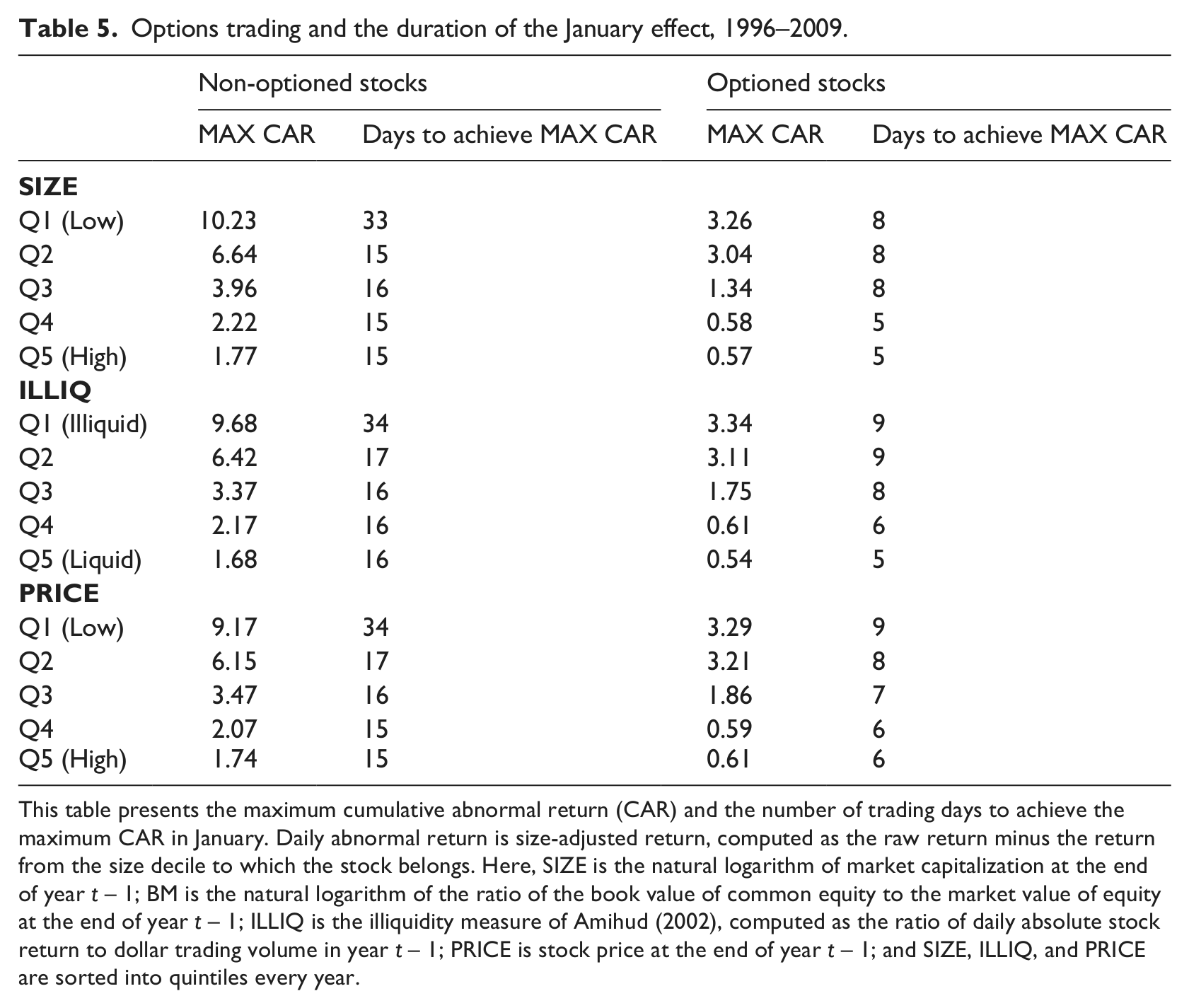
This table presents the maximum cumulative abnormal return (CAR) and the number of trading days to achieve the maximum CAR in January. Daily abnormal return is size-adjusted return, computed as the raw return minus the return from the size decile to which the stock belongs. Here, SIZE is the natural logarithm of market capitalization at the end of year t – 1; BM is the natural logarithm of the ratio of the book value of common equity to the market value of equity at the end of year t – 1; ILLIQ is the illiquidity measure of Amihud (2002), computed as the ratio of daily absolute stock return to dollar trading volume in year t – 1; PRICE is stock price at the end of year t – 1; and SIZE, ILLIQ, and PRICE are sorted into quintiles every year.

When we stratify the sample by quintiles of illiquidity or stock price, we also consistently find a lower maximum CAR value and a lower number of trading days to achieve the maximum CAR for optioned than for non-optioned stocks within each quintile of ILLIQ or PRICE. Taken together, the results in Table 5 suggest that the January effect is reduced and considerably more short lived among optioned than non-optioned stocks.

4.4. January risk-adjusted returns before and after an options listing

This section examines the effect of an options listing for a stock and its risk-adjusted return in January. We select a subsample of stocks optioned in the period 1998–2007 and compute risk-adjusted returns in January both after and before their options listing over the whole sample period 1996–2009. This ensures that there are at least two January observations before an options listing and two after the options listing for each firm.

Table 6 presents the results of this analysis. A total of 2127 stocks were optioned over the period 1998–2007. We first determine quintiles of SIZE by sorting stocks using the market capitalization at the end of the year before an options listing.¹¹ Within each SIZE quintile, we regress January risk-adjusted returns on a dummy variable (POST_LISTING) that takes a value of one if the return is after an options listing, and zero otherwise. In the lowest SIZE quintile, the coefficient on POST_LISTING is −2.36 and significant at the 1% level. This means that the January risk-adjusted return is 2.36% lower in the post-options-listing period than in the pre-options-listing period for a stock. The reduction in post-options-listing January risk-adjusted returns is also evident across other SIZE quintiles, although the effect decreases in firm size. When we sort stocks by ILLIQ or PRICE, we also find that the January risk-adjusted return is lower in the post-options-listing period and the effect is most pronounced for the most illiquid or the lowest-priced stocks.

Table 6.

Regression analysis of pre- and post-options-listing risk-adjusted returns in January, 1996–2009.

	Intercept	POST_LISTING
SIZE
Q1 (Low)	7.35	−2.36
	(4.20)	(−3.64)
Q2	5.62	−1.69
	(4.92)	(−3.49)
Q3	2.28	−0.91
	(2.95)	(−3.24)
Q4	1.29	−0.40
	(2.63)	(−2.16)
Q5 (High)	0.72	−0.13
	(1.42)	(−1.71)
ILLIQ
Q1 (Illiquid)	6.76	−2.02
	(4.79)	(−3.79)
Q2	4.87	−1.89
	(4.71)	(−4.69)
Q3	2.13	−1.91
	(3.11)	(−3.12)
Q4	1.18	−0.67
	(2.66)	(−2.31)
Q5 (Liquid)	0.79	−0.31
	(1.12)	(−0.77)
PRICE
Q1 (Low)	7.46	−2.42
	(4.10)	(−3.74)
Q2	4.12	−1.37
	(4.02)	(−3.57)
Q3	1.78	−0.57
	(2.55)	(−2.04)
Q4	1.19	−0.45
	(2.33)	(−1.16)
Q5 (High)	0.67	−0.17
	(1.42)	(−1.41)

This table presents the regression analysis of January risk-adjusted returns in the periods before and after an options listing. The sample comprises 2,127 firms optioned in 1998–2007. We use the Fama and French (1992) three-factor model in the five-year period leading to year t to estimate factor loadings and compute risk-adjusted returns for January stock returns in year t. Here, POST_LISTING is a dummy variable that takes a value of one if the January risk-adjusted return is before an options listing, and zero otherwise; SIZE is the natural logarithm of market capitalization at the end of the year before an options listing; ILLIQ is the illiquidity measure of Amihud (2002), computed as the ratio of daily absolute stock return to dollar trading volume in the year before an options listing; PRICE is stock price at the end of the year of an options listing; and SIZE, ILLIQ, and PRICE are sorted into quintiles every year. Heteroskedasticity-corrected t-statistics are in parentheses.

In summary, the results in Table 6 show the effect of an options listing in a longitudinal setting. There, we demonstrate that the phenomenon of higher stock returns in January is diminished once options trading is introduced for a stock.

4.5. Endogeneity and matched pair analysis

An issue inherent in the results of this study to consider is endogeneity. One may, for example, argue that optioned firms are large firms and high volatility firms which could possibly translate to lower January return. To correct for this endogeneity, we employ samples of matched firms and examine the January returns of optioned firms and matched firms in the pre-option-listing and post-option-listing periods.

We select three matched samples based on three matching procedures: (i) selecting a matched sample based on firm size and the magnitude of pre-options-listing January return, (ii) selecting a matched sample based on volatility and the magnitude of pre-options-listing January return, and (iii) selecting a matched sample based on the propensity score of having an option listing. The matched firm should not experience an option listing in the two years following the options listing of the optioned firm.

The first and second matching procedures go as follows. First, we compute the ranks of each matching variable firm size (or volatility) and pre-options-listing January return in an array formed by the optioned firm and all potential non-optioned matched firms. Second, we compute the absolute difference in ranks between the optioned firm and each of the potential non-optioned matched firms across the matching variables firm size (or volatility) and pre-options-listing January return. The non-optioned firm with the lowest sum of the two absolute rank differences is matched to the optioned firm. This procedure is repeated until we have matched pairs for all optioned firms.¹²

The third matching procedure is based on the ex-ante propensity of having an options listing (irrespective of the outcome).¹³ We first estimate each firm’s propensity of having an option listing by an individual propensity score. The propensity of options listing is determined by a probit model using a firm’s fundamental characteristics such as volume, volatility, and firm size that are relevant for exchange’s decision on an options listing (Mayhew and Mihov, 2004).¹⁴ In the second stage, firms are matched based on their closest propensity scores to determine the options listing outcome. Irrespective of the outcome, the control group firms are matched based on their nearest propensity of having an option listing. This matching technique helps address any selection bias from matching by firm characteristics.

Table 7 presents the results of this matched pair analysis. Panel A presents the results for optioned firms and non-optioned firms matched by pre-options-listing January return and volatility. The average volatility in the pre-options-listing period is 0.159 and 0.159 for optioned firms and non-optioned matched firms respectively. The average January return in the pre-options-listing period is 3.31 and 3.47 for optioned firms and non-optioned matched firms. The difference between optioned and non-optioned matched firms is insignificant, indicating a good match between the two samples. In the post-options-listing period, we note that the January return is 2.15 for optioned firms and 3.86 for non-optioned matched firms. The reduction of 1.16 in post-option-listing January return for optioned firms is significant at the 1 percent level. In contrast, non-optioned matched firms experience an increase of 0.36 in post-options-listing January return but this increase is not significant at the 1 percent level. The results in Panel A of Table 7 show that volatility remains almost unchanged for optioned and non-optioned firms in the post-options-listing period. January return, however, declines significantly for optioned firms in the post-options-listing period while such a finding is not evident among non-optioned matched firm.

Table 7.

Matched pair analysis, 1996–2009.

	Optioned firms	Matched non-optioned firms	Difference	Bootstrapped difference
Panel A: Matched by Pre-option-listing January Return and Volatility
Pre-options-listing Volatility	0.1595	0.1580	−0.0015(0.06)	−0.0009(0.507)
Post-options-listing Volatility	0.1603	0.0160	−0.0003(0.57)	−0.0002(0.88)
Difference	0.0008	0.0012
	(0.07)	(0.05)
Pre-options-listing January Return	3.31	3.47	0.16(0.24)	0.12(0.604)
Post-options-listing January Return	2.15	3.86	1.71(0.0001)	1.73(0.0001)
Difference	−1.16	0.36
	(0.0001)	(0.04)
Panel B: Matched by Pre-option-listing January Return and Firm Size
Pre-options-listing SIZE RANK	2.99	2.96	−0.03(0.89)	−0.02(0.82)
Post-options-listing SIZERANK	3.71	3.04	0.67(0.0001)	0.69(0.0001)
Difference	0.72	0.08
	(0.0001)	(0.42)
Pre-options-listing January Return	3.31	3.54	0.23(0.14)	0.19(0.56)
Post-options-listing January Return	2.15	3.69	1.54(0.0001)	1.50(0.0001)
Difference	−1.16	0.15
	(0.0001)	(0.07)
Panel C: Matched by Propensity Matching Score

Pre-options-listing January Return	3.31	4.17	0.86(0.0001)	0.85(0.0001)
Post-options-listing January Return	2.15	3.91	1.76(0.0001)	1.74(0.0001)
Difference	−1.16	−0.26
	(0.0001)	(0.10)

This table presents the analysis of options listing and January return from a matched pair approach. The optioned firm sample comprises 2,127 firms optioned in 1998–2007. In Panel A, each optioned firm is matched by a non-optioned firm by pre-options-listing January and volatility. In Panel B, each optioned firm is matched by a non-optioned firm by pre-options-listing January and SIZE. In Panel C, each optioned firm is matched by a non-optioned firm by the propensity of option listing score. Individual propensity to having an options listing is determined by a probit model with stock volume, volatility, and firm size as determinants of options listing (Mayhew and Mihov, 2004). Values in parentheses are p-values from Wilcoxon rank test for the difference. Bootstrapped difference is generated from 1000 re-sampling procedures with replacements.

Panel B of Table 7 presents the results for optioned firms and non-optioned firms matched by pre-options-listing January return and firm size. Pre-options-listing SIZERANK (in quintiles) is 2.99 and 2.96 for optioned firms and non-optioned matched firms, respectively. It is hence interesting to note that firms that experience an option listing are not necessarily very large firms as they are only slightly above the median firm size of the overall market. The pre-options-listing January return for non-optioned matched firms is 3.54. In the post-options-listing period, January return of non-optioned matched firms increases slightly to 3.69 and this increase is statistically insignificant. Thus, here we also document that non-optioned matched firms do not experience a reduction in January return as optioned firms do.¹⁵

Panel C of Table 7 presents the results for optioned firms and non-optioned firms matched by the propensity of having an options listing. Here, we find that non-optioned firms experience somewhat smaller January return in the post-options-listing period. However, the difference in January return between the pre- and post-options-listing periods of non-optioned matched firms is not statistically significant. The results here show the strongest evidence that reduced January return can be attributed to having an options listing outcome.

The last column in Table 7 presents bootstrapped difference between optioned and non-optioned firms from 1000 re-sampling procedures with replacements. Results from bootstrapped analysis generally support the main findings of Table 7 that there is a significant decline in the January return for optioned firms in the post-options-listing period while the January return is not noticeably different between the pre-options-listing period and the post-options-listing period for non-optioned matched firms.

5. Conclusions

Evidence of the January effect is still compelling, even though the investment community has been aware of this regularity in stock returns for several decades. The extant literature establishes that the January effect is mostly a small-stock phenomenon. Hence, trading costs and illiquidity have been suggested as the main impediments to investors wishing to exploit the January effect. This study proposes that options trading circumvents several limitations of trading in the equity market and facilitates exploiting the January effect. If this is the case, we expect that the January effect will diminish if options trading is readily available.

This study reports three significant findings. First, we find that risk-adjusted returns in January are significantly lower for optioned than for non-optioned stocks. In non-January months, however, we do not find an effect of options trading on stock returns. The effect of options trading on January stock returns cannot be attributed to other effects that have been documented in the literature as plausible explanations for the January phenomenon. Second, we find that the January effect is not only reduced but also more short-lived for optioned than for non-optioned stocks. Third, we show that January risk-adjusted returns are significantly lower in the post-options-listing period than in the pre-options-listing period of a stock.

Our study sheds new light on the implications of options trading for the equity market. We suggest that options trading allows investors to pursue trading strategies that may be economically infeasible in the equity market. Because there is a close link between stock and options prices, information from options trading will also be impounded into stock prices, which in turn improves the informational efficiency of the equity market.

Footnotes

Funding

This research received no specific grant from any funding agency in the public, commercial, or not-for-profit sectors.

Date of acceptance of final transcript: 1 February 2012.

Accepted by Associate Editor, Garry Twite (Finance).

Notes

References

Amihud

(2002) Illiquidity and stock return: Cross-section and time-series effects. Journal of Financial Markets 5: 31–56.

Amin

Lee

(1997) Option trading, price discovery, and earnings news dissemination. Contemporary Accounting Research 14: 153–192.

Athanassakos

(1992) Portfolio rebalancing and the January effect in Canada. Financial Analysts Journal 49: 67–78.

Back

(1993) Asymmetric information and options. Review of Financial Studies 6: 435–472.

Bhardwaj

Brooks

(1992) The January anomaly: Effects of low share price, transaction costs, and bid–ask bias. Journal of Finance 47: 553–576.

Biais

Hillion

(1994) Insider and liquidity trading in stock and options markets. Review of Financial Studies 7: 743–780.

Black

(1975) Fact and fantasy in the use of options. Financial Analysts Journal 31: 36–41.

Blume

Stambaugh

(1983) Biases in computed returns: An application to the size effect. Journal of Financial Economics 12: 387–404.

Branch

(1977) A tax-loss trading rule. Journal of Business 50: 198–207.

10.

Brown

Keim

Kleidon

. (1983) Stock return seasonalities and the tax-loss selling hypothesis: Analysis of the arguments and Australian evidence. Journal of Financial Economics 12: 105–127.

11.

Cao

Chen

Griffin

(2005) Informational content of option volume prior to takeovers. Journal of Business 78: 1072–1109.

12.

Cooper

Gulen

Rau

(2005) Changing names with style: Mutual fund name changes and their effects on fund flows. Journal of Finance 60: 2825–2858.

13.

Diamond

Verrecchia

(1987) Constraints on short-selling and asset price adjustment to private information. Journal of Financial Economics 18: 277–312.

14.

Duarte

Young

(2009) Why is PIN price? Journal of Financial Economics 91: 119–138.

15.

Dyl

(1977) Capital gains taxation and year-end stock market behavior. Journal of Finance 32: 165–175.

16.

Dyl

Maberly

(1992) Odd-lot transactions around the turn of the year and the January effect. Journal of Financial and Quantitative Analysis 27: 591–604.

17.

Easley

Hvidkjaer

O’Hara

(2002) Is information risk a determinant of asset returns? Journal of Finance 57: 2185–2221.

18.

Fama

French

(1992) The cross-section of expected stock returns. Journal of Finance 47: 427–466.

19.

Givoly

Ovadia

(1983) Year-end tax-induced sales and stock market seasonality. Journal of Finance 38: 171–185.

20.

Griffiths

White

(1993) Tax-induced trading and the turn-of-the-year anomaly: An intraday study. Journal of Finance 48: 575–598.

21.

Gultekin

(1983) Stock market seasonality: International evidence. Journal of Financial Economics 12: 469–481.

22.

Hakansson

(1982) Changes in the financial market: Welfare and price effects and the basic theorems of value conservation. Journal of Finance 37: 977–1004.

23.

Haug

Hirschey

(2006) The January effect. Financial Analysts Journal 62: 78–88.

24.

Haugen

Jorion

(1996) The January effect: Still there after all these years. Financial Analysts Journal 52: 27–31.

25.

Haugen

Lakonishok

(1988) The Incredible January Effect. Homewood, IL: Dow Jones Irwin.

26.

Wang

(2004) Quarterly trading patterns of financial institutions. Journal of Business 77: 493–509.

27.

Heckman

Ichimura

Todd

(1997) Matching as an econometric evaluation estimator: Evidence from evaluating a job training programme. Review of Economic Studies 64: 605–654.

28.

Heckman

Ichimura

Todd

(1998) Matching as an econometric evaluation estimator. Review of Economic Studies 65: 261–294.

29.

Hillion

Vermaelen

(2004) Death spiral convertibles. Journal of Financial Economics 71: 381–415.

30.

L-CJ

(1993) Option trading and the relation between price and earnings: A cross-sectional analysis. The Accounting Review 68: 368–384.

31.

Jennings

Starks

(1986) Earnings announcements, stock price adjustment, and the existence of option markets. Journal of Finance 41: 107–126.

32.

Kang

(2010) Probability of information-based trading and the January effect. Journal of Banking and Finance 34: 2985–2994.

33.

Kato

Schallheim

(1985) Seasonal and size anomalies in the Japanese stock market. Journal of Financial and Quantitative Analysis 20: 243–260.

34.

Keim

(1983) Size-related anomalies and stock return seasonality: Further empirical evidence. Journal of Financial Economics 12: 13–32.

35.

Koogler

Maberly

(1994) Additional evidence of year-end tax-motivated trading by individual investors, 1962–1986. Journal of the American Taxation Association 16: 122–137.

36.

Lakonishok

Shleifer

Thaler

. (1991) Window dressing by pension fund managers. American Economic Review 81: 227–231.

37.

Zhao

(2006) Propensity score matching and abnormal performance after seasoned equity offerings. Journal of Empirical Finance 13: 351–370.

38.

Liu

(2006) A liquidity-augmented capital asset pricing model. Journal of Financial Economics 82: 637–671.

39.

McConnell

(2008) Equity returns at the turn of the month. Financial Analyst Journal 64: 49–64.

40.

Manaster

Rendleman

Jr (1982) Option prices as predictors of equilibrium stock prices. Journal of Finance 37: 1043–1057.

41.

Maxwell

(1998) The January effect in the corporate bond market: A systematic examination. Financial Management 27: 18–30.

42.

Mayhew

Mihov

(2004) How do exchanges select stocks for option listing? Journal of Finance 59: 447–471.

43.

Mendenhall

Fehrs

(1999) Option listing and the stock-price response to earnings announcements. Journal of Accounting and Economics 27: 57–87.

44.

Moller

Zilca

(2008) The evolution of the January effect. Journal of Banking and Finance 32: 447–457.

45.

Musto

(1997) Portfolio disclosures and year-end price shifts. Journal of Finance 52: 1563–1588.

46.

Reinganum

(1983) The anomalous stock market behavior of small firms in January: Empirical tests for tax-loss selling effects. Journal of Financial Economics 12: 89–104.

47.

Ritter

(1988) The buying and selling behavior of individual investors at the turn of the year. Journal of Finance 43: 701–717.

48.

Rosenbaum

Rubin

(1983) The central role of the propensity score in observational studies for causal effects. Biometrika 70: 41–55.

49.

Ross

(1976) Options and efficiency. Quarterly Journal of Economics 90: 75–89.

50.

Rozeff

Kinney

Jr (1976) Capital market seasonality: The case of stock returns. Journal of Financial Economics 3: 379–402.

51.

Sias

Starks

(1997) Institutions and individuals at the turn-of-the-year. Journal of Finance 52: 1543–1562.

52.

Skinner

(1990) Options markets and the information content of accounting earnings releases. Journal of Accounting and Economics 13: 191–211.

53.

Stoll

Whaley

(1983) Transaction costs and the small firm effect. Journal of Financial Economics 12: 57–80.

54.

Tinic

Barone-Adesi

West

(1987) Seasonality in Canadian stock prices: A test of the “Tax-Loss-Selling” hypothesis. Journal of Financial and Quantitative Analysis 22: 51–64.

55.

Wachtel

(1942) Certain observations on seasonal movements in stock prices. Journal of Business 15: 184–193.

56.

Wilson

Jones

(1990) Is there a January effect in corporate bond and paper returns? Financial Review 25: 55–80.