An evaluation of the effectiveness of Value-at-Risk (VaR) models for Australian banks under Basel III

Abstract

This study compares Value-at-Risk (VaR) measures for Australian banks over a period that includes the Global Financial Crisis (GFC) to determine whether the methodology and parameter selection are important for capital adequacy holdings that will ultimately support a bank in a crisis period. VaR methodology promoted under Basel II was largely criticised during the GFC for its failure to capture downside risk. However, results from this study indicate that 1-year parametric and historical models produce better measures of VaR than models with longer time frames. VaR estimates produced using Monte Carlo simulations show a high percentage of violations but with lower average magnitude of a violation when they occur. VaR estimates produced by the ARMA GARCH model also show a relatively high percentage of violations, however, the average magnitude of a violation is quite low. Our findings support the design of the revised Basel II VaR methodology which has also been adopted under Basel III.

Keywords

Value-at-Risk (VaR)parametric VaR Monte Carlo simulation Basel Accords

1. Introduction

Value-at-Risk (VaR) is a risk measurement methodology that demonstrates the worst loss over a predetermined time horizon that will not be exceeded with a given level of confidence. See Jorion (2007) and Alexander (2008) for further explanation of the VaR measure. It allows the user to make a statement such as: this VaR figure is the maximum expected loss, with 99% confidence, in any one day. A VaR measurement is based on the examination of the percentiles of the distribution, summarising the downside risk of an institution due to financial market variables. This results in a single figure that is easy to interpret. VaR has a wide range of applications such as risk management and the determination of capital adequacy requirements.

Despite the apparent advantages of the ease of use of the VaR measurement it has been criticised in the literature and in practice predominantly due to unexpected extreme events, such as the Global Financial Crisis (GFC), which cause the distribution of asset returns to exhibit “fat tails”. Li (2013) reports concerns expressed by practitioners in regard to fat tails as revealed in interviews with bank risk managers relating to Basel II. Another apparent shortcoming of VaR is that it focuses on the probability of a loss, regardless of the magnitude of the violations when they do occur (see Basak and Shapiro, 2001; Berkowitz and O’Brien, 2002; Szegö, 2002). As Berkowitz and O’Brien (2002) demonstrated, although the violations of VaR in their dataset are infrequent, the magnitudes are surprisingly large.

The literature postulates new methodologies for calculating VaR. For example, Wang, Yeh and Cheng (2011) propose a new methodology specifically designed to examine tail risk. Gaglianone et al. (2011) also propose a new methodology for estimating VaR to identify periods of increased risk exposure. The CoVaR as initially proposed by Adrian and Brunnermeier (2011) and then empirically examined by Yun and Moon (2014) with Korean banking data is proposed to capture the systemic risk of financial institutions. As demonstrated by Li (2013), many practitioners also resort to other methods such as stress testing, Conditional VaR (CVaR) and Extreme Value Theory (EVT) as complementary approaches. However, the models that have persisted in the literature are the parametric approach, the historical approach and Monte Carlo simulations.

In Australia, VaR measures have been examined at the company, industry and market level using a variety of measurement techniques. Allen and Powell (2007) attempt to explain market risk at the industry level using VaR measures. Allen and Powell (2009b) examine the conditional credit VaR methodology. The authors then use this methodology to allow banks to incorporate industry risk using the relationship between market and credit risk. Allen and Powell (2009a), and Allen et al. (2012b) use the conditional credit VaR methodology to examine market risk from an Australian sectoral perspective and explain banks’ equity fluctuations prior to and during the financial crisis. Allen et al. (2012a) present a comparative analysis of conditional autoregressive VaR models with other volatility models such as GARCH (1,1).

Much of the literature on VaR focuses on US and European commercial banks, see for example Berkowitz and O’Brien (2002), Cuoco and Liu (2006), Lucas (2001), Fiori and Iannotti (2007), Pérignon et al. (2008) and Pérignon and Smith (2010a, 2010b), Berkowitz et al. (2011) to name a few. This is expected given the importance of the VaR calculation for commercial banks under the Basel Accords. Berkowitz and O’Brien (2002) provide a particularly interesting insight into VaR calculations using proprietary profit and loss information of six large US banks. They use a 99 percent historical model and compare this with an ARMA GARCH model. Results of this research show that the ARMA GARCH model is better able to adjust to changes in volatility. More recently, studies have begun to show that there can be significant variation in results using different approaches to calculating VaR. For example, Kim et al. (2011) compare backtests of VaR ARMA GARCH models and produce similar results with Berkowitz and O’Brien (2002). Using an Asian hedge fund index, Weng and Trück (2011) suggest that a parametric model outperforms the historical approach but that GARCH models are among the best. In addition, Da Veiga et al. (2011) show different performances of five volatility models used to forecast VaR thresholds.

This paper assesses and compares a number of different measurement approaches including parametric, historical, Monte Carlo simulations and ARMA GARCH to examine VaR measures based on returns of the nine largest banks in Australia. The study includes the Global Financial Crisis, during which time widespread VaR measures were highly criticised. This research has implications for the capital adequacy standards as it compares different methodologies that could be used to calculate VaR measures using banks that performed relatively well during the financial crisis.

This paper is organised as follows. Section 2 outlines the basic types of VaR models, Section 3 describes the application of VaR measurement to the Basel II and III Accords, Section 4 provides a discussion of the data and methodology and the results are presented in Section 5. Section 6 provides a summary.

2. Theoretical assessment of basic VaR models

VaR models may be categorised into four groups of analytic techniques.¹ First, the parametric approach calculates the historical standard deviation and then scales the appropriate factors; second, the historical approach directly reads the quantile from the historical distribution; third, Monte Carlo simulation estimates VaR from repeatedly simulated prices or returns of the financial instrument; and, fourth, the ARMA GARCH model is used to estimate the mean and variance of the distribution which can then be used to estimate the VaR.

Parametric VaR models, in contrast to the nonparametric category, attempt to fit a parametric distribution such as a normal distribution to the data. Specifically, the models are applied to portfolios assuming that returns are independent and identically distributed with a normal distribution including portfolios of cash, futures and/or forward positions on commodities, bonds, loans, swaps,² equities and foreign exchange (Alexander, 2008).

The historical method uses the empirical quantile of the historical distribution of return series in a very direct way as a guide to what might happen in the future. The main advantage of the historical method is that it makes no assumptions about risk factor changes being from a particular distribution. By relying on actual prices, this method allows nonlinearities and non-normal distributions. It does not rely on specific assumptions about valuation models or the underlying stochastic structure of the market. The historical method is therefore able to reliably predict the VaR as shown by Winker and Maringer (2007), but they also find a substantial amount of hidden risk when it is used for a risk constraint in portfolio optimisation.

Monte Carlo simulation is a flexible and powerful methodology that has numerous applications to finance including VaR estimation. It is a process of repeatedly simulating the prices or returns of financial instruments or portfolios, to be confident that the simulated distribution of portfolio values is sufficiently close to the “true” distribution of actual portfolio values, which is used as a reliable proxy. VaR then can be estimated from this proxy distribution (see Alexander, 2008; Dowd, 2005; Ganegoda and Evans, 2014; Jorion, 2007). However, its computational time is a major drawback, consequently it is often too expensive to implement on a frequent basis. Also, the potential of model risk cannot be ignored, because Monte Carlo relies on specific stochastic processes for the underlying risk factors as well as the pricing model for securities such as options or mortgages. For further details, see Jorion (2007).

With ARMA and GARCH methodology, an ARMA model is used to estimate the mean of the distribution and a GARCH model is used to calculate the volatility of the distribution. These parameters are then used as inputs in the VaR calculation. ARMA methodology is frequently used in forecasting time series models with considerable accuracy, particularly in the short term. ARMA combines two different specifications into one equation, an autoregressive (AR) process and a moving average (MA) process. The AR process includes past values of the dependent variable while the MA process includes past error terms. Hence, an ARMA(1,1) process includes only the most recent past values of the dependent variable and the most recent error term in the regression equation. The GARCH methodology of Bollerslev (1986) is an adaptation of the Auto Regressive Conditional Heteroskedasticity model (ARCH) (Engle, 1982) known as the Generalised ARCH model. As discussed in Vlaar (2000) and Sjölander (2009) GARCH modelling is used to model the time-varying volatility of financial assets, which in practice is possible to limit the number of lagged squared disturbance terms and conditional variances to one, resulting in a GARCH(1,1) model.

3. VaR application in Basel II and III

In the field of prudential supervision, VaR has been embraced as the fundamental market risk measurement methodology to calculate regulatory capital under the Basel Accords. Basel II in particular promotes further application and dramatic development of VaR models. The Basel Committee suggests calculating VaR on a daily basis at the 99 percent level with a one-tailed confidence interval; the historical observation period is “constrained to be a minimum length of one year” (Basel Committee on Banking Supervision (BCBS), 2006).

Banks are required to ensure that their internal models have been adequately validated by conducting regular backtesting over the recent 250 days under Basel II. Described as a procedure of “reality checks” by Jorion (2007), backtesting tests whether realised (current) exposures are consistent with the shortcut method prediction over all margin periods within one year (BCBS, 2006), to prove the model validation to supervisors. If the actual loss occurred on a day is greater than the VaR estimation for that day, an “exception” is recorded.

The Basel Committee requires banks to meet minimum capital requirement for their market risk exposures based on VaR estimations, multiplied by a multiplication factor. The multiplication factor is set on the basis of banks’ model validation assessment: VaR backtesting. Backtesting here refers to a comparison of the VaR measures that were used compared with the actual number of exceptions that were identified over that period. If the number of exceptions from VaR backtesting during the previous 250 days is less than 5 which falls in the “green zone”, the multiplication factor k is normally set equal to 3. If number of exceptions is 5, 6, 7, 8 and 9 which fall in the “yellow zone”, the multiplication factor is set equal to 3.4, 3.5, 3.65, 3.75 and 3.85, respectively. A multiplication factor of 4 is set for the “red zone” in which the number of exceptions equals to 10 or more (BCBS, 2006). As specified in the Basel II Accord (BCBS, 2006), the green zone corresponds to backtesting results that do not themselves suggest a problem with the quality or accuracy of a bank’s VaR models; the yellow zone encompasses results that do raise questions on models’ quality or accuracy; the red zone indicates a problem with a bank’s VaR models according to backtesting result.

The empirical effectiveness of VaR models based on the above criterion has been evaluated in the literature. Brummelhuis and Kaufmann (2007) evaluate the time scaling of VaR estimations using the square-root-of-time rule as specified in Basel II and conclude that the rule performs reasonably well. Sjölander (2009) compares VaR models with shorter estimation periods with the 1-year minimum estimation period required by Basel II. The study finds that out-of-sample risk predictions are more accurate when using shorter estimation periods. Gürtler et al. (2010) compare VaR and expected shortfall models in relation to their suitability in assessing the concentration of the risk of credit portfolios according to the Basel II requirements. Their results highlight the accuracy of VaR for measuring the concentration risk of credit portfolios.

Research on the empirical performance of VaR measures also includes those that evaluate the validity requirements in Basel II, such as Kerkhof and Melenberg (2004), Kerkhof et al. (2010), Kaplanski and Levy (2007), De la Pena et al. (2006), Dowd (2006) and Hurlin and Tokpavi (2006). These studies analyse the range of the backtesting penalty structures (as described above) with multiplication factors.

Studies on VaR models published before the Global Financial Crisis, such as Alexander and Baptista (2006) warn that the use of VaR under Basel II may increase financial market fragility. They suggest that certain banks will select riskier portfolios when a VaR constraint is imposed under the Basel Accords. They suggest that inaccurate risk assessments based on VaR may lead to excessive risk exposures and capital charges that are consequently not sufficient to absorb the losses. In addition, Haq et al. (2014) and Hoang et al. (2013) provide support for the argument that current capital requirements are not sufficient to offset bank’s post-GFC risk taking activities. They suggest that the increased risk is mainly due to the provision of government safety nets.

The GFC featured the failure of financial institutions including commercial banks (see Alali and Romero, 2013). This triggered a revision of Basel II’s VaR-based market risk framework to address extreme events. The Basel Committee set up some more restrictive requirements in the revision, however the VaR methodology itself remains unchanged in the Basel II revision. This means the features and parameters of VaR methodologies as described above, have not been changed under the Basel II revision. In accordance with the Basel III structure, the Basel Committee has kept the VaR methodology intact while the reviewing continues (BCBS, 2011).

The number of ongoing studies testing VaR models has increased following the GFC, due to the repercussions for financial institutions that miscalculated risk exposures. For example, Kim et al. (2011) backtest VaR models based on different distributional assumptions during GFC and investigate the difference between VaR values for normal models compared with non-normal models including ARMA GARCH models which are proven to be the best among the models they investigated. Pesaran and Pesaran (2010) examine asset return correlations during the GFC and the ability of VaR models to characterise market risk. The study concludes that VaR models fail diagnostic testing when applied to the post-2007 period. Zhao et al. (2010) introduce a new approach for estimating VaR, which is then used to show the likelihood of the impacts of the current financial crisis. The model is shown to have the capability to reliably estimate such likelihood on stock and index returns. Obi et al. (2010) examine the market risk exposure of investments in the South African stock market during the GFC using VaR as a measure of market risk. This study shows that the model is a better reflection of the true impact of market risk under volatile conditions. McAleer et al. (2013) investigate the performance of a variety of single and combined VaR forecasts in terms of daily capital requirements and violation penalties under Basel II. They present evidence to support the claim that the median point forecast of VaR is generally robust to events such as the GFC.

Under Basel II, its revision and Basel III, the VaR methodology itself has been continuously applied either for supervisory purposes or for banks’ internal risk management without major amendments. Therefore, it is important to evaluate the accuracy and effectiveness of VaR models using Australian bank data, given that the Australian banking sector performed relatively well during the GFC having implemented Basel II principles at an early stage.

4. Data and methodology

The daily share prices for the largest nine banks in Australia by market capitalisation were collected from Datastream for the full time period available for each bank up to 30 June 2011. Comparative analysis includes data for the period 1 July 2001 to 30 June 2011.

Table 1 provides return statistics for each of the banks over their full history. Consistent with the approach by Gupta and Liang (2005), we have applied VaR methodology to daily share price returns. This approach circumvents several problems in calculating VaR including the proprietary nature of profit and loss information, the complex portfolio structure of major banks and the inclusion of nonlinear assets such as options and interest rate derivatives commonly held by large commercial banks.

Table 1.

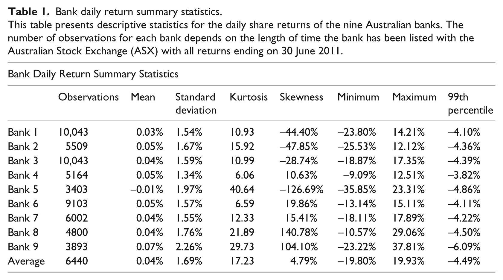
Bank daily return summary statistics.

This table presents descriptive statistics for the daily share returns of the nine Australian banks. The number of observations for each bank depends on the length of time the bank has been listed with the Australian Stock Exchange (ASX) with all returns ending on 30 June 2011.

Bank Daily Return Summary Statistics
	Observations	Mean	Standard deviation	Kurtosis	Skewness	Minimum	Maximum	99th percentile
Bank 1	10,043	0.03%	1.54%	10.93	−44.40%	−23.80%	14.21%	−4.10%
Bank 2	5509	0.05%	1.67%	15.92	−47.85%	−25.53%	12.12%	−4.36%
Bank 3	10,043	0.04%	1.59%	10.99	−28.74%	−18.87%	17.35%	−4.39%
Bank 4	5164	0.05%	1.34%	6.06	10.63%	−9.09%	12.51%	−3.82%
Bank 5	3403	−0.01%	1.97%	40.64	−126.69%	−35.85%	23.31%	−4.86%
Bank 6	9103	0.05%	1.57%	6.59	19.86%	−13.14%	15.11%	−4.11%
Bank 7	6002	0.04%	1.55%	12.33	15.41%	−18.11%	17.89%	−4.22%
Bank 8	4800	0.04%	1.76%	21.89	140.78%	−10.57%	29.06%	−4.50%
Bank 9	3893	0.07%	2.26%	29.73	104.10%	−23.22%	37.81%	−6.09%
Average	6440	0.04%	1.69%	17.23	4.79%	−19.80%	19.93%	−4.49%

The approach in this study also follows the workings of Berkowitz and O’Brien (2002), which focuses on bank VaR estimates using a parametric model with 99 percent confidence, consistent with the Basel II and III requirements. In this study we also use a 1-year, 3-year, 5-year, 7-year and 10-year time frame to determine the parameters of μ and σ, where

VaR = μ - 2.33 σ

for a 99 percent parametric model, μ is the the mean of the daily share price returns and σ is the standard deviation of the daily share price returns.

In this study we also use the historical approach to calculate VaR. Using this approach we calculate the lowest 1 percentile loss in daily returns. A 1-year, 3-year, 5-year, 7-year and 10-year time frame is again used to calculate the VaR. These VaR measures are then compared to the return that is realised on the following day. Therefore, all comparison are out-of sample.

Monte Carlo simulations are used to generate share returns using formula provided in Boyle (1977), namely

S_{t + 1} = S_{t} \exp [r - σ^{2} / 2 + σ \tilde{x}]

where S_t is the the current stock price at time t, r is the risk-free rate of return, σ is the standard deviation of the stock price returns and $\tilde{x}$ is a normally distributed random variable with zero mean and unit variance.

In addition, the antithetic variate method, as described by Boyle (1977), is used as a variance reduction technique to reduce simulation error. Five thousand simulated pathways are derived for the bank share prices, followed by 5000 simulated pathways where the random numbers generated are the negative of the first 5000 random numbers. The returns generated using the Monte Carlo simulations are then used to estimate VaR by examining the lowest quantile of returns from the simulated distribution. This measure of VaR is compared with the current return, so that all comparisons are out-of-sample.

We also use an ARMA(1,1) plus GARCH(1,1) model of share returns as an alternative VaR model as suggested by Berkowitz and O’Brien (2002). The reduced form model of r_t _{+ 1} is estimated by

r_{t + 1} = μ + ρ {rt + u}_{t + 1} + λ u_{t}

(1)

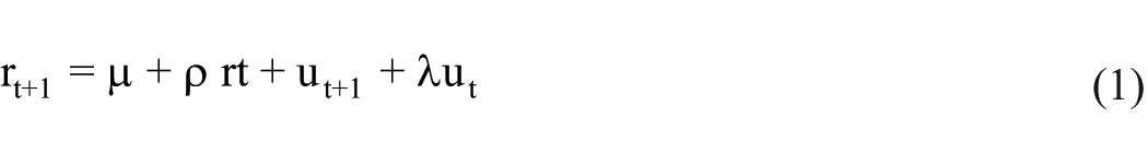
where u_t₊₁ is an independent and identically distributed (i.i.d.) innovation with mean zero and variance σ²_t. The volatility process σ²_t+1 is described by

σ_{t + 1}^{2} = ω + θ u_{t}^{2} + σ_{t}^{2}

(2)

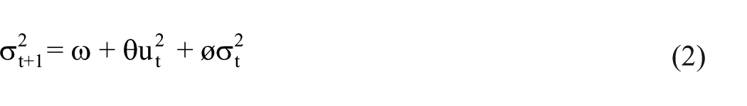
where ω, θ and ø are parameters to be estimated. We apply the standard GARCH model where innovations are assumed to be conditionally normal. Thus, the 99 percent VaR forecast at time t is given by ŕ_t₊₁ – 2.33ờ_t+1, where ŕ_t₊₁ is the predicted value of r_t₊₁ from equation (1) and ờ_t+1 is the estimated standard deviation from equation (2).

Assessment of each of the models is conducted out of sample. Therefore, there are no forecasts for the first 260 days, with forecasts thereafter using only information that would have been available on that day to calculate VaR. VaR estimates are calculated every day thereafter. The sample size is different for each of the banks due to the availability of historical share prices. This process forms the basis for our model validation.

As described by Dowd (2005), model validation involves applying statistical methods to determine whether the forecasts of a VaR model are consistent with the model assumptions. This process may also be used to compare different models that may be used for VaR forecasts. Model validation is considered vital to making a judgement on the performance of risk models. Hence, this approach is adopted in this paper in two ways. First, the bank’s share returns are examined to assess the normality or otherwise of the distribution. Second, model validation is used to compare the parametric, historical, Monte Carlo simulation and ARMA GARCH models. This process of out of sample forecast evaluation is also known as backtesting. As explained by Alexander (2008) failure of a backtest indicates VaR model misspecification and/or large estimation errors. A Kupiec measure is calculated to evaluate whether the number of exceptions is statistically significantly different to what would be expected. This method was first introduced by Kupiec (1995), stating that the number of exceptions should follow a binomial distribution, where the probability of experiencing x exceptions is

\Pr (x | n, p) = (_{x}^{n}) p^{x} {(1 - p)}^{n - x}

where x is the number of exceptions, n is the number of trials and p is the probability of an exception for a given confidence interval. The figures shown in the results tables are the p-value associated with the test, whereby a figure less than 0.05 indicates that the number of exceptions is not consistent with the binomial distribution.

5. Results

Summary statistics are reported in Table 1 for each of the nine banks daily share price returns representing the profits and losses for these banks. The length of time varies from 3403 trading days to 30 June 2011 to 10,043 trading days to 30 June 2011. Table 1 shows that eight of the nine banks had positive average returns following the bank’s listing, with a minimum daily return of −35.85% and a maximum daily return of 37.81%. The highest standard deviation was 2.26% and the lowest standard deviation was 1.34%.

Histograms of the daily share price returns are presented in Figure 1. These figures also incorporate the measures of kurtosis and skewness as shown in Table 1. The kurtosis and skewness estimates (relative to the normal distribution) displayed in columns 5 and 6 appear to be quite large. This is reflected in the histograms of daily share price returns and is consistent with previous research such as that by Lucas (2001) and Cuoco and Liu (2006).

Figure 1.

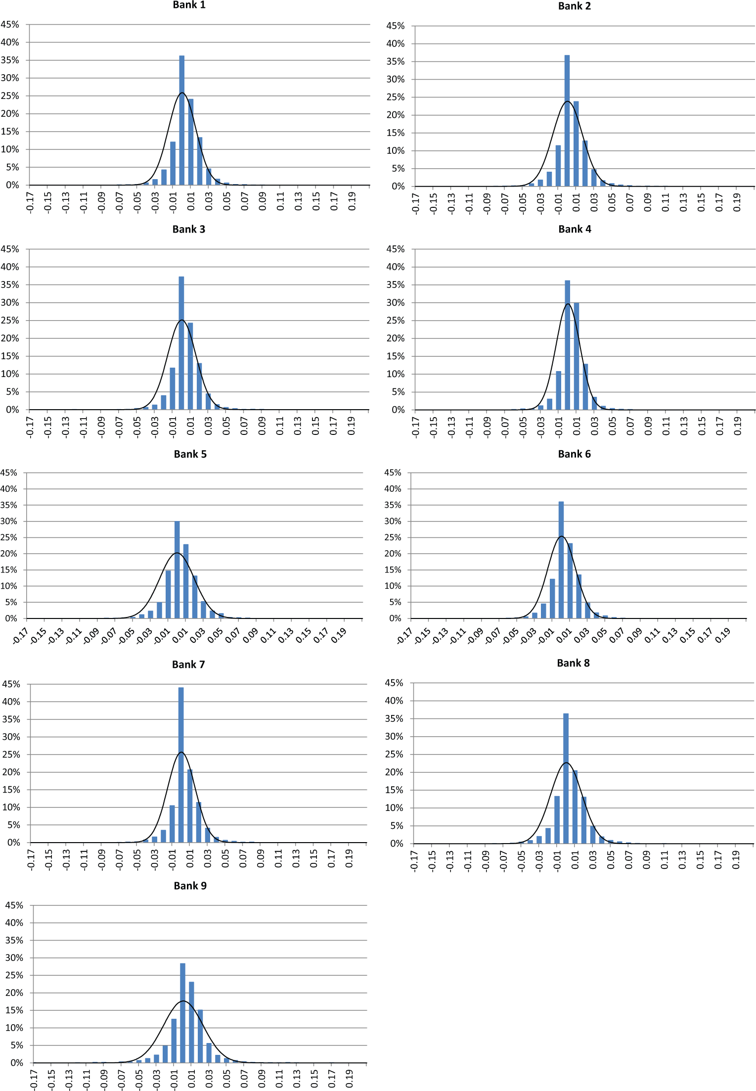
Bank daily return distributions.

Table 2 provides the results of the analysis of a 99% 1-year VaR parametric model. It shows that the losses are occurring about 1.78 of every 100 days for these large commercial Australian banks. This appears to be a high number of violations as we would expect 1 violation in every 100 days. However, this result is consistent with prior literature such as Pérignon et al. (2008) and Berkowitz and O’Brien (2002) which shows that VaR estimates are higher than expected and higher than proves to be the case. These research papers postulate an understatement of the diversification benefits achieved by banks investing in a wide range of assets. However, Pérignon and Smith (2010a, 2010b) further investigate the reasons behind the high VaR estimates and shows that the diversification benefits are not understated by the banks. In addition, as discussed in Section 4, this result of 1.78 violations in every 100 days would be considered to be in the green zone under the Basel III methodology. This methodology suggests that a model is in the “green zone”, acceptable level, if the number of exceptions from VaR backtesting during the previous 250 days is less than 5. Our results fall in this category.

Table 2.

Summary of bank 99% 1-year VaR parametric models.

This table presents the results of the 99% 1 year parametric VaR model. The number of observations is less than the total number of observations presented in Table 1 as the model uses the first year of returns to estimate the VaR measure to be compared with the subsequent actual return. Mean VaR shows the average VaR estimate for each bank based on a 99% 1-year parametric model. The number (%) of violations represents the number (%) of times the actual return on a given day is lower than the VaR estimate for that day. The mean violation shows the average exceedance of the actual share return below the VaR estimate when a violation occurs. The Kupiec measure shows the p-value associated with the Kupiec (1995) test which demonstrates whether the number of violations is statistically significantly different to the number of violations expected from a 99% model.

	Observations	Mean VaR	Number of violations	Percentage of violations	Mean violation	Kupiec
Bank 1	9782	−3.42%	171	1.75%	−1.29%	0.0000
Bank 2	5249	−3.56%	99	1.89%	−1.18%	0.0000
Bank 3	9782	−3.43%	164	1.68%	−1.64%	0.0000
Bank 4	4903	−2.91%	86	1.75%	−1.09%	0.0000
Bank 5	3142	−4.37%	65	2.07%	−1.67%	0.0000
Bank 6	8842	−3.45%	169	1.91%	−1.12%	0.0000
Bank 7	5741	−3.40%	99	1.72%	−1.23%	0.0000
Bank 8	4539	−3.89%	75	1.65%	−0.93%	0.0000
Bank 9	3631	−4.67%	57	1.57%	−2.04%	0.0003
Average	6179	−3.68%	109	1.78%	−1.35%

Column 6 of Table 2 shows mean violation, which suggests that when a loss does occur the daily return is on average 1.35% below the estimated VaR. Figures 2 and 3 provide a graphical representation of this information. Figure 2 shows the daily returns for each of the banks along with the VaR estimate for each day. Figure 3 isolates each violation of VaR. These figures show the timing of each of the violations of VaR and the magnitude of each violation. Figures 2 and 3 show that the largest violation was for bank 5, which experienced a violation of VaR by approximately 30% in June 2003. This event clearly influenced the kurtosis and skewness estimates for bank 5 as shown in Table 1. The Kupiec test in column 7 of Table 2 attempts to determine whether the observed number of violations of the model is consistent with the expected number of violations. The null hypothesis is that the model is correct and with such low p-values we can reject this null hypothesis for each of the banks using this test.

Figure 2.

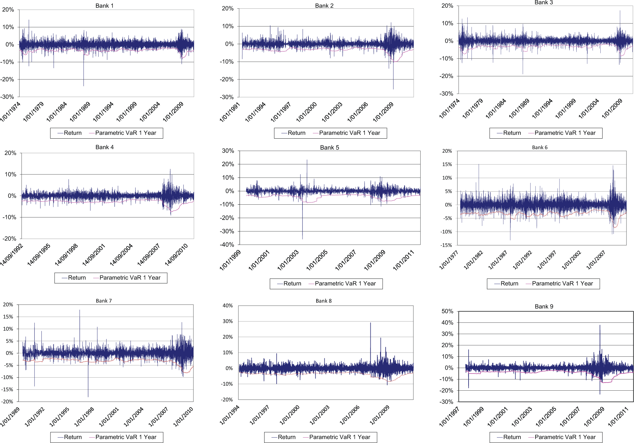
Bank daily VaR models.

Figure 3.

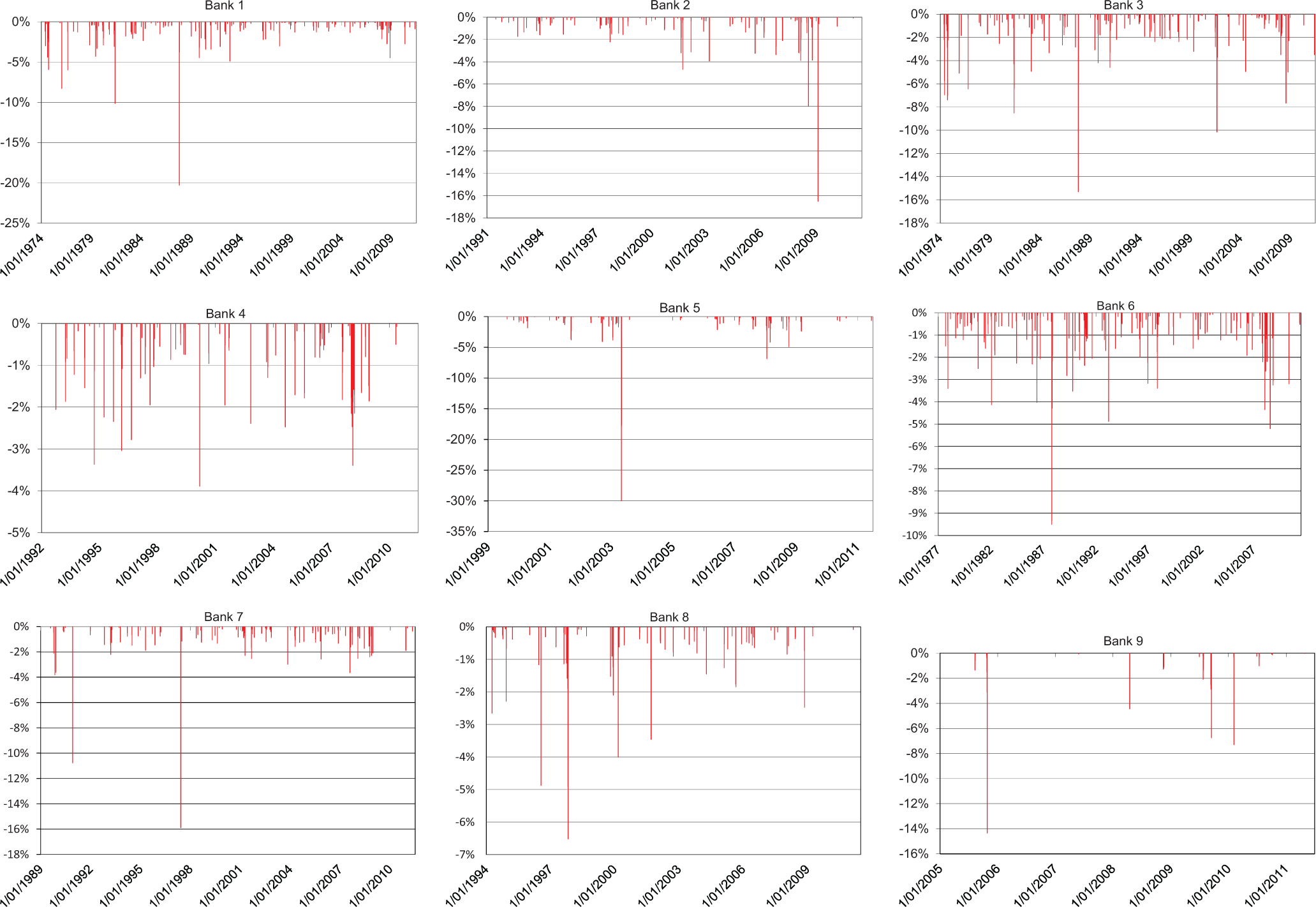
Bank daily 99% VaR violations.

Table 3 provides a comparison of parametric VaR models using different lengths of time to estimate μ and σ. Column 5 shows that 1 year model has the lowest percentage of violations and column 6 shows that the 1-year model also has the lowest mean violation when such an event occurs. However, it is likely that our results are influence by events at the time of the GFC. During this time large and expected negative returns occurred. Models with longer time horizons took longer to incorporate this new information. However, the models with a shorter time horizon were faster to respond to the changing economic conditions incorporating larger VaRs, as shown in column 3 of Table 3. Using the Kupiec test we can reject the null hypothesis that this is the correct model for each of the banks using the parametric VaR model. This result is consistent with the findings of Sjölander (2009), which shows that shorter estimation periods produce better out of sample risk predictions.

Table 3.

Comparison of parametric bank VaR models.

This table presents the results of 99% parametric VaR models with varying estimation periods. Mean VaR shows the average VaR estimate for each bank based on each model. The number (%) of violations represents the number (%) of times the actual return on a given day is lower than the VaR estimate for that day. The mean violation shows the average exceedance of the actual share return below the VaR estimate when a violation occurs. The Kupiec measure shows the p-value associated with the Kupiec (1995) test which demonstrates whether the number of violations is statistically significantly different to the number of violations expected from a 99% model.

	Observations	Mean VaR	Number of violations	Percentage of violations	Mean violation
Average 1-year	6179	−3.68%	109	1.78%	−1.35%
Average 2-year	5921	−3.75%	108	1.85%	−1.42%
Average 3-year	5655	−3.76%	112	2.04%	−1.49%
Average 4-year	5386	−3.71%	114	2.20%	−1.53%
Average 5-year	5128	−3.79%	100	2.11%	−1.52%
Average 6-year	4868	−3.76%	94	2.11%	−1.55%
Average 7-year	4614	−3.64%	103	2.36%	−1.52%
Average 8-year	4355	−3.76%	90	2.38%	−1.62%
Average 9-year	4092	−3.66%	98	2.75%	−1.55%
Average 10-year	3824	−3.69%	93	2.84%	−1.59%

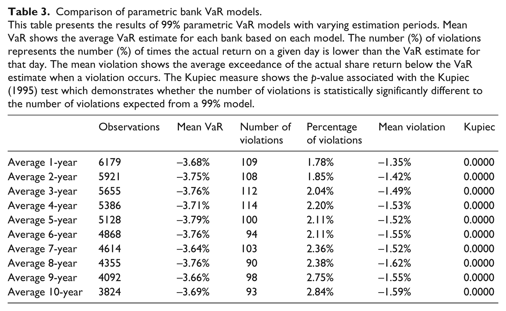
Table 4 provides an analysis of a 99% 1-year VaR historical model. It shows that the losses are occurring 1.47 in every 100 days for each these large commercial Australian banks. Column 3 of Table 4 shows that that the average VaR for the banks is −3.92% which is more negative than that of the equivalent parametric model in Table 2. Column 5 of Table 4 shows that there was an average of 1.47% violations which is lower than the parametric model however, it is still above the expected 1% or 1 in 100 days. Column 6 of Table 4 shows that when a loss does occur it is on average 1.41% below the estimated VaR, only slightly higher than that of the parametric model. Using the Kupiec test we can reject the null hypothesis that this is the correct model for 8 of the 9 banks at the 1% level.

Table 4.

Summary of bank 99% 1-year VaR historical models.

This table presents the results of the 99% 1-year historical VaR model. Mean VaR shows the average VaR estimate for each bank based on a 99% 1-year parametric model. The number (%) of violations represents the number (%) of times the actual return on a given day is lower than the VaR estimate for that day. The mean violation shows the average exceedance of the actual share return above the VaR estimate when a violation occurs. The Kupiec measure shows the p-value associated with the Kupiec (1995) test which demonstrates whether the number of violations is statistically significantly different to the number of violations expected from a 99% model.

	Observations	Mean VaR	Number of violations	Percentage of violations	Mean violation	Kupiec
Bank 1	9782	−3.77%	136	1.39%	−1.35%	0.0000
Bank 2	5249	−3.82%	75	1.43%	−1.41%	0.0006
Bank 3	9782	−3.88%	130	1.33%	−1.81%	0.0003
Bank 4	4903	−3.12%	71	1.45%	−0.98%	0.0006
Bank 5	3142	−4.54%	56	1.78%	−1.64%	0.0000
Bank 6	8842	−3.77%	136	1.54%	−1.13%	0.0000
Bank 7	5741	−3.63%	89	1.55%	−1.19%	0.0000
Bank 8	4539	−3.96%	67	1.48%	−1.01%	0.0005
Bank 9	3631	−4.78%	46	1.27%	−2.18%	0.0177
Average	6179	−3.92%	90	1.47%	−1.41%

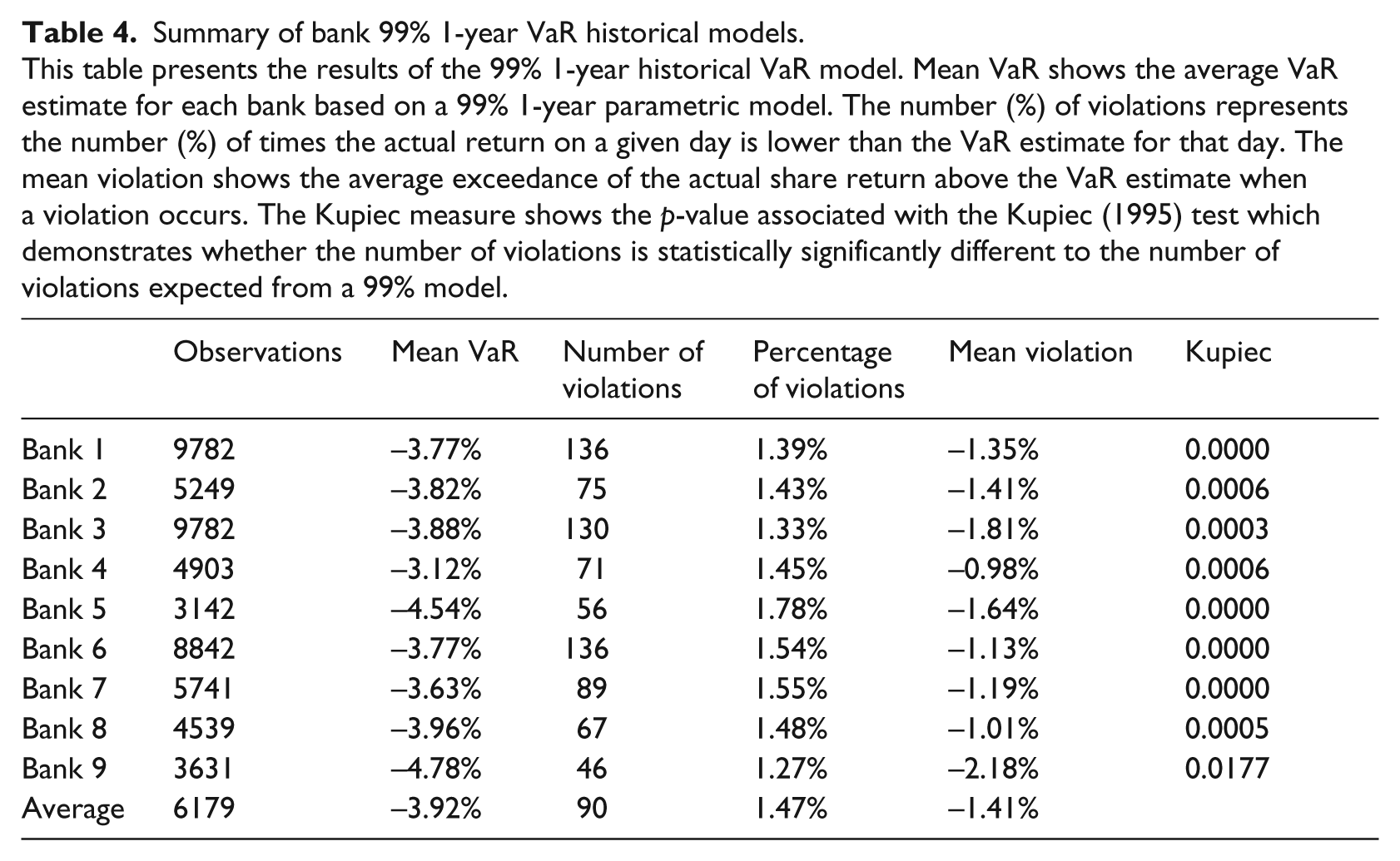
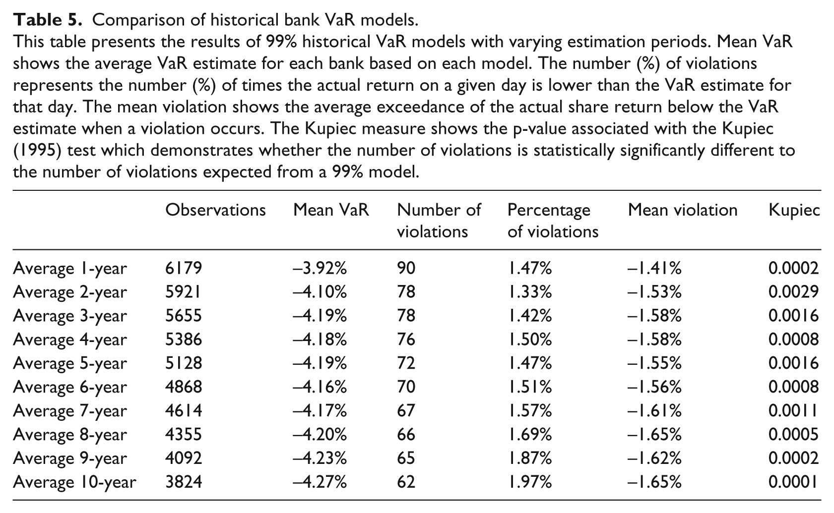
Table 5 provides a comparison of historical VaR models using different lengths of time. Column 5 shows that the 1-year model has a relatively low percentage of violations and column 6 shows that the 1-year model has the lowest mean violation when such an event occurs. This is consistent with Table 3 and is likely to be influence by the GFC. However, this table also shows that the lower level of violations is able to be achieved without larger VaR estimates. This suggests that by adapting more quickly to the economic conditions lower levels of violations can occur by raising the VaR estimates when conditions are good and lowering VaR estimates when conditions are poor. Using the Kupiec test we can reject the null hypothesis that this is the correct model for each of the banks at the 1% level.

Table 5.

Comparison of historical bank VaR models.

This table presents the results of 99% historical VaR models with varying estimation periods. Mean VaR shows the average VaR estimate for each bank based on each model. The number (%) of violations represents the number (%) of times the actual return on a given day is lower than the VaR estimate for that day. The mean violation shows the average exceedance of the actual share return below the VaR estimate when a violation occurs. The Kupiec measure shows the p-value associated with the Kupiec (1995) test which demonstrates whether the number of violations is statistically significantly different to the number of violations expected from a 99% model.

	Observations	Mean VaR	Number of violations	Percentage of violations	Mean violation	Kupiec
Average 1-year	6179	−3.92%	90	1.47%	−1.41%	0.0002
Average 2-year	5921	−4.10%	78	1.33%	−1.53%	0.0029
Average 3-year	5655	−4.19%	78	1.42%	−1.58%	0.0016
Average 4-year	5386	−4.18%	76	1.50%	−1.58%	0.0008
Average 5-year	5128	−4.19%	72	1.47%	−1.55%	0.0016
Average 6-year	4868	−4.16%	70	1.51%	−1.56%	0.0008
Average 7-year	4614	−4.17%	67	1.57%	−1.61%	0.0011
Average 8-year	4355	−4.20%	66	1.69%	−1.65%	0.0005
Average 9-year	4092	−4.23%	65	1.87%	−1.62%	0.0002
Average 10-year	3824	−4.27%	62	1.97%	−1.65%	0.0001

Berkowitz and O’Brien (2002) suggest that high correlations across banks may be a potential concern to bank supervisors because it raises the spectre of systematic risk, that is, the simultaneous realisation of large losses at several banks. Table 6 shows the correlations between the nine Australian bank’s daily share price returns and their VaR estimates, with t-statistics shown in parentheses. Panel A of Table 6 shows that the correlations between the bank’s daily share price returns are all positive but generally quite low, ranging from 0.35 to 0.73 with an average of 0.49. The associated t statistics are shown in parenthesis. None of the correlations are significant at the 10% level. This is consistent with the finding of Berkowitz and O’Brien (2002) suggesting that this reflects some differences in portfolio compositions among banks. Panel B of Table 6 shows the correlations for daily VaR across the nine banks. The correlations are consistently positive and relatively high, ranging from 0.38 to 1.00 with an average of 0.85. All correlations are significant at the 1% level. These correlations show the similarities in bank VaRs in Figure 2 and are consistent with the positive correlations of the daily share price return between the nine banks.

Table 6.

Correlations of bank returns and VaR across individual banks.

This table presents the correlation between the daily share returns for each bank (Panel A) and the VaR estimates (Panel B) across individual banks. The figures shown are the Pearson correlation and the associated t-statistic in parentheses.

Panel A: Return correlation coefficients
	Bank 1	Bank 2	Bank 3	Bank 4	Bank 5	Bank 6	Bank 7	Bank 8	Bank 9
Bank 1	1.00
Bank 2	0.51 (–48.82)	1.00
Bank 3	0.64 (–25.06)	0.47 (41.00)	1.00
Bank 4	0.71 (31.61)	0.47 (62.43)	0.68 (49.44)	1.00
Bank 5	0.42 (–38.96)	0.40 (–11.95)	0.43 (–27.03)	0.42 (–43.05)	1.00
Bank 6	0.73 (–21.26)	0.47 (59.94)	0.70 (16.11)	0.68 (–47.3)	0.42 (31.34)	1.00
Bank 7	0.45 (–59.67)	0.37 (7.41)	0.48 (–31.02)	0.46 (–73.49)	0.35 (15.26)	0.47 (–42.48)	1.00
Bank 8	0.42 (–44.41)	0.39 (–6.59)	0.44 (–31.89)	0.45 (–52.4)	0.35 (7.54)	0.44 (–37.11)	0.44 (–17.04)	1.00
Bank 9	0.48 (–55.81)	0.47 (–45.53)	0.56 (–56.06)	0.49 (–60.75)	0.43 (–10.51)	0.54 (–62.26)	0.41 (–36.4)	0.43 (–26.92)	1.00
Panel B: VaR correlation coefficients
	Bank 1	Bank 2	Bank 3	Bank 4	Bank 5	Bank 6	Bank 7	Bank 8	Bank 9
Bank 1	1.00
Bank 2	0.97 (–0.87)	1.00
Bank 3	0.97 (–0.96)	0.96 (0.11)	1.00
Bank 4	0.99 (–0.06)	0.98 (0.82)	0.99 (0.98)	1.00
Bank 5	0.59 (–1.28)	0.55 (–0.46)	0.53 (–0.6)	0.57 (–1.27)	1.00
Bank 6	0.99 (–0.13)	0.98 (0.74)	0.99 (0.91)	1.00 (–0.07)	0.58 (1.18)	1.00
Bank 7	0.94 (–0.09)	0.96 (0.66)	0.94 (0.66)	0.94 (–0.05)	0.42 (1.09)	0.95 (0.00)	1.00
Bank 8	0.82 (0.04)	0.84 (0.76)	0.84 (0.73)	0.82 (0.08)	0.38 (1.16)	0.84 (0.12)	0.90 (0.12)	1.00
Bank 9	0.96 (–0.09)	0.96 (0.58)	0.96 (0.54)	0.96 (–0.06)	0.52 (0.95)	0.97 (–0.02)	0.96 (–0.02)	0.90 (–0.12)	1.00

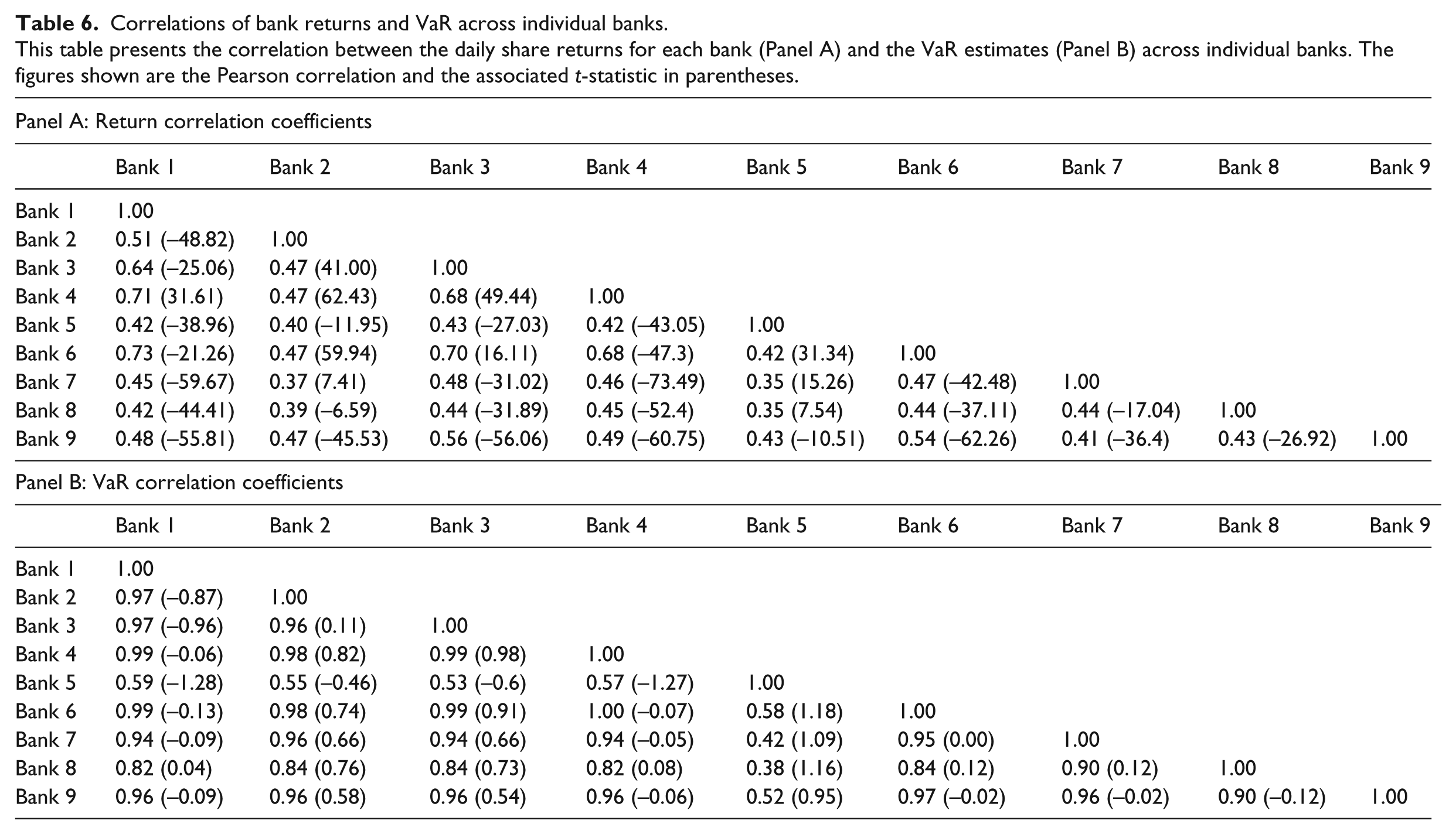
Table 7 demonstrates the VaR estimates produced by the model using Monte Carlo simulations. Column 5 shows a higher average percentage of violations than would be expected under a 99% model at 2.00%. This is higher than both the parametric model and historical models which had an average percentage violation of 1.78% and 1.47%, respectively, over the same period. Column 3 shows that this was at least partly due to a higher VaR estimate. The mean VaR estimate for Monte Carlo simulations was −3.52% compared with −3.68% (−3.92%) for the parametric (historical) models. Column 5 shows that the Monte Carlo simulation model has the lowest level of violations at −1.32% when a violation does occur, compared with the parametric (−1.35%) and historical (−1.41%) models. This demonstrates that even though the Monte Carlo Simulation model is a more sophisticated method of calculating VaR it does not necessarily provide better estimates for Australian banks and produces similar results to the other methods. Using the Kupiec test we can reject the null hypothesis that this is the correct model for all of the 9 banks at the 1% level.

Table 7.

Backtests of Monte Carlo simulation VaR model.

This table presents the results of the VaR model produced using Monte Carlo simulations. Mean VaR shows the average VaR estimate for each bank based on the Monte Carlo simulation model. The number (%) of violations represents the number (%) of times the actual return on a given day is lower than the VaR estimate for that day. The mean violation shows the average exceedance of the actual share return below the VaR estimate when a violation occurs. The Kupiec measure shows the p-value associated with the Kupiec (1995) test which demonstrates whether the number of violations is statistically significantly different to the number of violations expected from a 99% model.

	Observations	Mean VaR	Number of violations	Percentage of violations	Mean violation	Kupiec
Bank 1	9781	−3.28%	193	1.97%	−1.26%	0.0000
Bank 2	5247	−3.41%	111	2.12%	−1.19%	0.0000
Bank 3	9781	−3.29%	185	1.89%	−1.57%	0.0000
Bank 4	4902	−2.79%	93	1.90%	−1.11%	0.0000
Bank 5	3141	−4.17%	71	2.26%	−1.68%	0.0000
Bank 6	8841	−3.31%	184	2.08%	−1.15%	0.0000
Bank 7	5740	−3.26%	112	1.95%	−1.21%	0.0000
Bank 8	4538	−3.72%	86	1.90%	−0.94%	0.0000
Bank 9	3631	−4.44%	71	1.96%	−1.80%	0.0000
Average	6178	−3.52%	123	2.00%	−1.32%

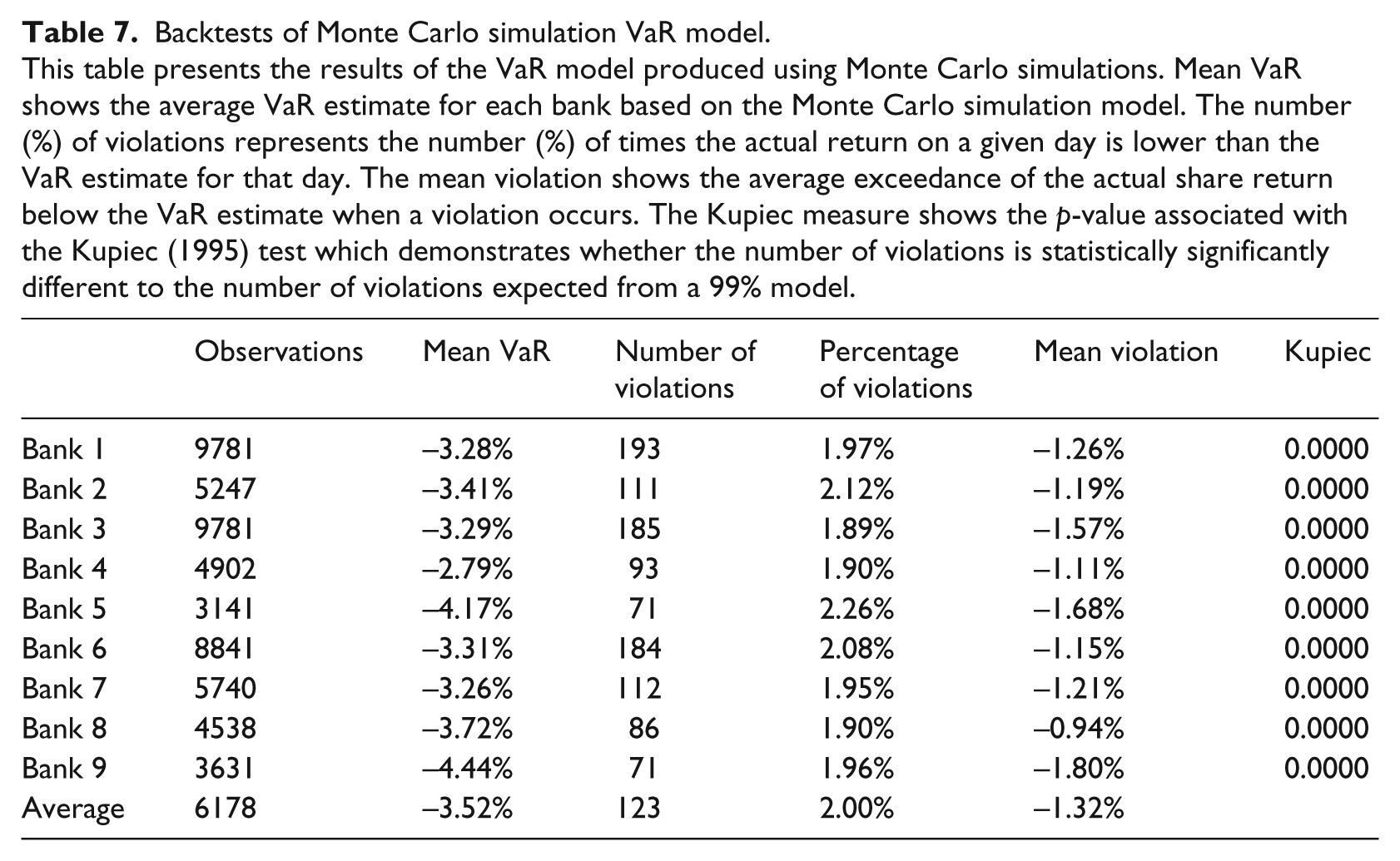
Table 8 demonstrates the VaR estimates produced by the ARMA GARCH model. Consistent with the other methodologies tested, column 5 shows an average percentage of violations higher than would be expected under a 99% model at 1.79%. This is similar to the percentage of violations by the parametric model at 1.78% over the same period. Column 3 shows that the higher level of violations occurred even though this model produced a lower VaR estimate. The mean VaR estimate for the ARMA GARCH model was −3.59% compared with −3.52% for the Monte Carlo simulations, −3.68% for the parametric model and −3.92% for the historical method. Column 6 shows that the ARMA GARCH model has the lowest level of violations, when a violation occurs, at −1.15% compared with the parametric (−1.35%), historical (−1.41%) and Monte Carlo simulation (−1.32%) models. This demonstrates that the sophisticated methodology of the ARMA GARCH model produces a relatively large percentage of violations, however the magnitude of violations, when they occur, are relatively low. This result was achieved through relatively low levels of VaR. Using the Kupiec test we can reject the null hypothesis that this is the correct model for each of the banks at the 1% level.

Table 8.

Backtests of ARMA(1,1) + GARCH(1,1) VaR model.

This table presents the results of the ARMA GARCH VaR model. Mean VaR shows the average VaR estimate for each bank based on the ARMA GARCH model. The number (%) of violations represents the number (%) of times the actual return on a given day is lower than the VaR estimate for that day. The mean violation shows the average exceedance of the actual share return below the VaR estimate when a violation occurs. The Kupiec measure shows the p-value associated with the Kupiec (1995) test which demonstrates whether the number of violations is statistically significantly different to the number of violations expected from a 99% model.

	Observations	Mean VaR	Number of violations	Percentage of violations	Mean violation	Kupiec
Bank 1	9783	−3.35%	164	1.68%	−1.11%	0.0000
Bank 2	5249	−3.55%	89	1.70%	−1.18%	0.0000
Bank 3	9783	−3.31%	194	1.98%	−1.14%	0.0000
Bank 4	4904	−2.84%	88	1.79%	−0.78%	0.0000
Bank 5	3143	−4.35%	61	1.94%	−1.67%	0.0000
Bank 6	8843	−3.39%	165	1.87%	−0.98%	0.0000
Bank 7	5742	−3.31%	99	1.72%	−1.09%	0.0000
Bank 8	4540	−3.84%	81	1.78%	−0.82%	0.0000
Bank 9	3633	−4.40%	60	1.65%	−1.59%	0.0001
Average	6180	−3.59%	111	1.79%	−1.15%

Overall, the ARMA GARCH model appears to offer the best results when compared with parametric, historical and Monte Carlo simulation models. The ARMA GARCH model demonstrates a relatively low violation level when such an event occurs, which appears to be achieved without estimating lower levels of VaR. This result is consistent with Berkowitz and O’Brien (2002), Kim et al. (2011) and Weng and Trück (2011).

6. Conclusion

This study examines different methodologies and parameter selection for calculating VaR measures, including those adopted under the Basel II Accords and subsequently Basel III. The Basel VaR methodology was heavily criticised during the GFC due to its inability to account for downside risk, following the failure of some key financial institutions. This study focuses on VaR measures for Australian banks, which were particularly resilient GFC.

Consistent with prior literature, such as studies by Lucas (2001) and Cuoco and Liu (2006), analysis of the daily share price returns shows that the kurtosis and skewness estimates, relative to the normal distribution, appear to be quite large. Analysis of a 99% 1-year VaR parametric model shows that losses are occurring about 1.78 of every 100 days for each these nine large commercial Australian banks. When a loss does occur it is on average 1.35% below the estimated VaR. The largest violation of VaR was by approximately 30% in June 2003. This event clearly influenced the kurtosis and skewness estimates for the return distribution of this bank.

A comparison of parametric VaR models using different lengths of time to estimate the VaR measure show that the 1-year model has the lowest percentage of violations and the lowest mean violation when such an event occurs, a result that is consistent with Sjölander (2009). It is likely that the results are influence by events at the time of the Global Financial Crisis. During this time large and unexpected negative returns occurred. Models with longer time horizons took longer to incorporate this new information. However, models with a shorter time horizons were faster to respond to the changing economic conditions, producing more negative VaR’s at crucial times. This is consistent with the findings using historical VaR models. However, the lower level of violations is able to be achieved without lower overall VaR estimates on average. This suggests that by adapting more quickly to the economic conditions lower levels of violations can occur by raising the VaR estimates when conditions are good and lowering VaR estimates when conditions are poor.

Our research findings support the VaR methodology adopted under the Basel II revision and Basel III as the 99% 1-year historical model incorporates new information quickly into the VaR calculation. Consistent with Berkowitz and O’Brien (2002), Kim (2011) and Weng and Trück (2011) the more sophisticated models appear to add sufficient improvement to justify the additional resources required to run such models. This information is relevant in relation to the banking sector for further policy-making purpose and the design of internal models.

Footnotes

Acknowledgements

We thank the referee, Tom Smith, Paul Docherty, Daniel Smith and other participants at the Queensland University of Technology seminar, participants at the University of Newcastle seminar and an anonymous referee for helpful comments and suggestions. We also thank Professor Hiroshi Takamori, Professor Megumi Suto and other participants at the Finance Research Center seminar of the Waseda University for their suggestions.

Final transcript accepted 28 September 2014 by Tom Smith (AE Finance).

Funding

This research received no specific grant from any funding agency in the public, commercial, or not-for-profit sectors.

Notes

References

Adrian

Brunnermeier

(2011) CoVaR. NBER Working Paper No. 17454. Cambridge, MA: National Bureau of Economic Research.

Alali

Romero

(2013) Characteristics of failed U.S. commercial banks: An exploratory study. Accounting and Finance 53: 1149–1174.

Alexander

(2008) Value-at-Risk Models: Market Risk Analysis, vol. IV. Hoboken, NJ: John Wiley & Sons Ltd.

Alexander

Baptista

(2006) Does the Basel Capital Accord reduce bank fragility? An assessment of the value-at-risk approach. Journal of Monetary Economics 53: 1631–1660.

Allen

Powell

(2007) Industry market value at risk in Australia. FEMARC Working Paper Series 0704. Joondalup WA: Edith Cowan University.

Allen

Powell

(2009a) Structural credit modelling and its relationship to market value at risk: An Australian sectoral perspective. In: Gregoriou

(ed.) The VAR Implementation Handbook. New York: McGraw-Hill, pp. 403–414.

Allen

Powell

(2009b) Transitional credit modelling and its relationship to market value at risk: An Australian sectoral perspective. Accounting and Finance 49: 425–444.

Allen

Singh

Powell

(2012a) A Gourmet’s delight: CAViaR and the Australian stock market. Applied Economic Letters 19: 1493–1498.

Allen

Singh

Powell

(2012b) The fluctuating default risk of Australian banks. Australian Journal of Management 37: 297–325.

10.

Basak

Shapiro

(2001) Value-at-risk-based risk management: Optimal policies and asset price. Review of Financial Studies 14: 371–450.

11.

Basel Committee on Banking Supervision (BCBS) (2006) Basel II: International Convergence of Capital Measurement and Capital Standards—A Revised Framework. Basel, Switzerland: Bank for International Settlements.

12.

Basel Committee on Banking Supervision (BCBS) (2011) Basel III: A Global Regulatory Framework for More Resilient Banks and Banking System. Basel, Switzerland: Bank for International Settlements.

13.

Berkowitz

O’Brien

(2002) How accurate are value-at-risk models at commercial banks. Journal of Finance 57: 1093–1111.

14.

Berkowitz

Christoffersen

Pelletier

(2011) Evaluating value-at-risk models with desk-level data. Management Science 15: 2213–2227.

15.

Bollerslev

(1986) Generalized autoregressive conditional heteroskedasticity. Journal of Econometrics 31: 307–327.

16.

Boyle

(1977) Options: A Monte Carlo approach. Journal of Financial Economics 4: 323–338.

17.

Brummelhuis

Kaufmann

(2007) Time-scaling of value-at-risk in GARCH(1,1) and AR(1)-GARCH(1,1) processes. Journal of Risk 9: 39–94.

18.

Cuoco

Liu

(2006) An analysis of VaR-based capital requirements. Journal of Financial Intermediation 15: 362–394.

19.

Da Veiga

Chan

McAleer

(2011) It pays to violate: How effective are the Basel accord penalties in encouraging risk management. Accounting and Finance 52: 95–116.

20.

De la Pena

Rivera

Ruiz-Mata

(2006) Quality control of risk measures: Backtesting VAR models. Journal of Risk 9: 39–54.

21.

Dowd

(2005) Measuring Market Risk. 2nd ed. Hoboken, NJ: John Wiley & Sons Ltd.

22.

Dowd

(2006) Backtesting market risk models in a standard normality framework. Journal of Risk 9: 93–111.

23.

Engle

(1982) Autoregressive conditional heteroscedasticity with estimates of variance of United Kingdom inflation. Econometrica 50: 987–1008.

24.

Fiori

Iannotti

(2007) Scenario-based principal component value-at-risk when the underlying risk factors are skewed and heavy-tailed: An application to Italian banks’ interest rate risk exposure. Journal of Risk 9: 63–99.

25.

Gaglianone

Lima

Linton

. (2011) Evaluating value-at-risk models via quantile regression. Journal of Business & Economic Statistics 29: 150–160.

26.

Ganegoda

Evans

(2014) A framework to manage the measurable, immeasurable and the unidentifiable financial risk. Australian Journal of Management 39: 5–34.

27.

Gupta

Liang

(2005) Do hedge funds have enough capital? A value-at-risk approach. Journal of Financial Economics 77: 219–253.

28.

Gürtler

Hibbeln

Vöhringer

(2010) Measuring concentration risk for regulatory purposes. Journal of Risk 12: 69–104.

29.

Haq

Faff

Seth

. (2014) Disciplinary tools and bank risk exposure. Pacific-Basin Finance Journal 26: 37–64.

30.

Hoang

Faff

Haq

(2013) Market discipline and bank risk taking. Australian Journal of Management 39: 327–350.

31.

Hurlin

Tokpavi

(2006) Backtesting value-at-risk accuracy: A simple new test. Journal of Risk 9: 19–37.

32.

Jorion

(2007) Value at Risk: The New Benchmark for Managing Financial Risk. 3rd ed. New York: MaGraw-Hill.

33.

Kaplanski

Levy

(2007) Basel’s value-at-risk capital requirement regulation: An efficiency analysis. Journal of Banking & Finance 31: 1887–1906.

34.

Kerkhof

Melenberg

(2004) Backtesting for risk-based regulatory capital. Journal of Banking & Finance 28: 1845–1865.

35.

Kerkhof

Melenberg

Schumacher

(2010) Model risk and capital reserves. Journal of Banking & Finance 34: 267–279.

36.

Kim

Rachev

Bianchi

. (2011) Time series analysis for financial market meltdowns. Journal of Banking & Finance 35: 1879–1891.

37.

Kupiec

(1995) Techniques for verifying the accuracy of risk management models. Journal of Derivatives 3: 73–84.

38.

(2013) Risk Management and Regulatory Features of Basel II and Basel III for Smart Banking Management. Hershey, PA: IGI Global Publishing.

39.

Lucas

(2001) Evaluating the Basel guidelines for backtesting banks’ internal risk management models. Journal of Money, Credit and Banking 33: 826–846.

40.

McAleer

Jiménez-Martín

Pérez-Amaral

(2013) International evidence on GFC-robust forecasts for risk management under the Basel accord. Journal of Forecasting 32: 267–288.

41.

Obi

Sil

Jeong-Gil

(2010) Value-at-risk with time varying volatility in South African equities. Journal of Global Business & Technology 6: 1–11.

42.

Pérignon

Smith

(2010a) Diversification and value-at-risk. Journal of Banking & Finance 34: 55–56.

43.

Pérignon

Smith

(2010b) The level and quality of value-at-risk disclosure by commercial banks. Journal of Banking & Finance 34: 362–377.

44.

Pérignon

Deng

Wang

(2008) Do banks overstate their value-at-risk. Journal of Banking & Finance 32: 783–794.

45.

Pesaran

(2010) Conditional volatility and correlations of weekly returns and the VaR analysis of 2008 stock market crash. Economic Modelling 27: 1398–1416.

46.

Sjölander

(2009) Are the Basel II requirements justified in the presence of structural breaks? Applied Financial Economics 19: 985–998.

47.

Szegö

(2002) Measures of risk. Journal of Banking & Finance 26: 1253–1272.

48.

Vlaar

(2000) Value at risk models for Dutch bond portfolios. Journal of Banking & Finance 24: 1131–1154.

49.

Wang

Yeh

Cheng

(2011) How accurate is the square-root-of-time rule in scaling tail risk: A global study. Journal of Banking & Finance 35: 1158–1169.

50.

Weng

Trück

(2011) Style analysis and value-at-risk of Asia-focused hedge funds. Pacific-Basin Finance Journal 19: 491–510.

51.

Winker

Maringer

(2007) The hidden risks of optimizing bond portfolios under VaR. Journal of Risk 9: 1–19.

52.

Yun

Moon

(2014) measuring systemic risk in the Korean banking sector via dynamic conditional correlation models. Pacific-Basin Finance Journal 27: 94–114.

53.

Zhao

Scarrott

Oxley

. (2010) Extreme value modelling for forecasting market crisis impacts. Applied Financial Economics 20: 63–72.