Social capital and idiosyncratic return volatility

Abstract

We examine whether regional social capital has any impact on idiosyncratic return volatility. Using US data, we find that firms headquartered in high social capital counties exhibit significantly lower idiosyncratic return volatility. This effect is more pronounced in the presence of financial reporting quality and corporate social responsibility. When we estimate the direct and indirect effects of social capital, our study reveals that the direct effect of social capital captures around 80% of the total effect. These findings suggest that firm-specific variables do not explain all of a firm’s idiosyncratic return volatility, but regional social capital also plays a role.

JEL classification: G10, G12, G30, M14

Keywords

Corporate social responsibility financial reporting quality idiosyncratic return volatility social capital

1. Introduction

Idiosyncratic return volatility (IRV) constitutes the largest component of risk in an individual stock, and it has valuable implications for portfolio analysis, asset pricing, valuation of employee stock options and managerial compensation policies (e.g. Goyal and Santa-Clara, 2003; Liu and Di lorio, 2016; March and Shapira, 1987; Morck et al., 2013; Nartea et al., 2011). Therefore, the determinants of IRV have received considerable research interest in the finance and accounting literature.

In this article, we examine whether county-level social capital in the United States affects the IRV of firms headquartered in those counties. Social capital ‘… is an instantiated informal norm that promotes co-operation between two or more individuals’ (Fukuyama, 2001: 7). Recent studies in the area of finance and accounting show that firms headquartered in high social capital counties are associated with more socially responsible behaviour (Jha and Cox, 2015), lower bank loan spreads (Hasan et al., (2017a)), lower corporate tax avoidance (Hasan et al., (2017b)) and lower audit fees (Jha and Chen, 2015). An important, yet unexplored issue is whether county-level social capital reduces investors’ uncertainty about future cash flows and return. Therefore, this study explores the effect of social capital on firm-level IRV and the channels through which the relationship, if any, manifests itself.

There remains divergence of opinion as to whether IRV represents market efficiency or risk. Proponents supporting the former argue that higher IRV represents incorporation of more firm-specific information into stock prices, thus making stock price more informative (Dasgupta et al., 2010; Fox et al., 2003). Risk-based arguments, however, propose that cash flow uncertainty and deteriorating financial reporting quality (FRQ) have been primarily responsible for a surge in the IRV which is detrimental to shareholders’ value (Irvine and Pontiff, 2009; Rajgopal and Venkatachalam, 2011). Consistent with this argument, Ang et al. (2006) document that stocks in the bottom quintile of IRV outperform stocks in the top quintile by more than 1% per month. Pontiff (2006) contends that IRV is the single largest cost faced by arbitrageurs resulting from noise trading. Consistent with the risk-based explanation of IRV, we contend that IRV increases investors’ valuation risk and hence investigate whether the social capital of the counties in which firms are headquartered reduces such risk.

Traditional asset pricing theory contends that investors can diversify IRV by holding a portfolio of stocks and therefore such risk is not priced in equilibrium (McAlister et al., 2007; Nartea et al., 2011). However, studies indicate that investors, in reality, may not hold perfectly diversified portfolios for several reasons, including (1) transaction and search costs associated with a diversified portfolio (Ang et al., 2006; Merton, 1987); (2) attraction towards stocks with certain characteristics such as higher volatility, higher market beta, higher skewness and higher turnover (Goetzmann and Kumar, 2008); (3) excessive exposure to a single firm; (4) ‘erroneous’ diversification strategy (Goetzmann and Kumar, 2008) and (5) investor sophistication and investor-specific attributes (Dorn and Huberman, 2005). Given that under-diversification exposes investors to high IRV, the largest source of riskiness of the stock – understanding the determinants of IRV – is crucial for maximizing investors’ wealth. Extant literature documents that information asymmetry generates heterogeneous beliefs among investors about future cash flows and return, which in turn influence IRV (Chen et al., 2012; Rajgopal and Venkatachalam, 2011). An improvement in the quality of corporate disclosures and financial reporting can mitigate such information asymmetries, leading to a reduction in uncertainties and, hence, IRV (Diamond and Verrecchia, 1991; Healy et al., 1999). In the context of social capital, prior research has found that the ‘cooperative norms’ aspect of social capital constrains opportunistic behaviours in transactions (Coleman, 1988), while ‘density in social networks’ fosters an environment for effective communication and enforcement of deviant behaviour (Guiso et al., 2004) – in our case, financial reporting manipulation and pro-active corporate social responsibility (CSR) behaviour. Therefore, we argue that the prevalent social capital enhances FRQ, thereby reducing information asymmetry and the associated return volatility. We also consider firms’ involvement in CSR as another channel through which social capital reduces the IRV. Jha and Cox (2015) show that firms from high social capital counties exhibit higher CSR, implying that the altruistic inclination of the region in which a firm is headquartered plays an important role in explaining firms’ involvement in CSR. Extant studies also show that ‘relational wealth’ emanating from CSR provides insurance-like protection and reduces cash flow uncertainty and thus IRV (Luo and Bhattacharya, 2009; Mishra and Modi, 2013). Since firms headquartered in high social capital counties exhibit more CSR, we expect the cooperative norm, dense network and relational wealth stemming from social capital and CSR to help the firm develop a bulwark against future loss of economic value, which is likely to reduce risk, vulnerability of future cash flows and thus IRV.

Since social capital affects FRQ and CSR, and both FRQ and CSR affect the IRV, we expect social capital to play a more dominant role when interacted with FRQ or CSR. Therefore, in the regression analysis, we interact social capital with FRQ or CSR to examine the association between social capital and IRV. Additionally, to isolate the extent to which social capital directly and indirectly (through FRQ or CSR) affects IRV, we use the simultaneous equations model.

Our primary measures of social capital are two variants of social norms and two measures of networks (Rupasingha and Goetz, 2008). Using these four indicators, Rupasingha and Goetz (2008) conducted a principal component analysis for each year (1997, 2005 and 2009) and used the first component for each year as the social capital index. Recent finance and accounting studies (e.g. Hasan et al., (2017a, 2017b); Jha and Chen, 2015; Jha and Cox, 2015) use the same index as a proxy for social capital. A linear interpolation fills the missing years. As is consistent with prior research, we measure IRV as the standard deviation of the residuals from the asset pricing models.

Using a comprehensive sample during the period 1997–2014, we document a negative and significant effect of social capital on IRV after controlling for firm characteristics, county-level demographic factors, and year and industry effects. Our results suggest that a firm headquartered in a county with social capital in the 75th percentile is associated with 24% less IRV compared to a firm headquartered in a county with social capital in the 25th percentile. We also find that FRQ and CSR moderate the relationship between social capital and IRV. Importantly, when we isolate the direct and indirect effects of social capital on IRV, we find that the direct effect of social capital captures around 80% of the effects. Our findings are robust to alternative specifications of social capital and IRV, and to the use of two-stage least squares analysis to alleviate the endogeneity concern.

Our study contributes to the literature in a number of important ways. First, we present evidence of the effect of social capital on IRV, which has not been documented before. Extant studies (e.g. Goyal and Santa-Clara, 2003; Lui et al., 2007) document that IRV accounts for more than 80% of the variation in a firm’s stock risk. Given that individual investors are largely undiversified (Goetzmann and Kumar, 2008), it is important to understand the determinants of this risk – social capital, in our setting. To the best of our knowledge, this is the first study to introduce social capital into the IRV literature. Second, we contribute to the nascent literature on the effects of social capital on corporate financial outcomes. Although Guiso et al. (2004) suggest that social capital entails positive economic outcomes, very few studies have investigated the effect of social capital on corporate decisions (Hasan et al., (2017a, 2017b); Jha, (2017); Jha and Chen, 2015; Jha and Cox, 2015 are exceptions). Our study fills this gap in the literature. Third, we enrich the CSR literature by incorporating social capital into the CSR domain. Although prior evidence reveals that firms headquartered in high social capital counties engage more in positive CSR activities (Jha and Cox, 2015) and CSR activities also reduce IRV (Luo and Bhattacharya, 2009), the extent to which social capital-induced CSR activities affect IRV remains unexplored.

The remainder of the article proceeds as follows. In Section 2, we review the related literature and develop our hypotheses. Section 3 describes the research design, followed by Section 4 describing the descriptive statistics. Section 5 reports the results. Section 6 concludes the article.

2. Literature review and hypotheses development

Idiosyncratic risk reflects firm-specific return volatility, which results primarily from a firm’s actions and is independent of the common market movement. Interestingly, prior studies consistently document that idiosyncratic risk, rather than market risk, constitutes the largest component of variation (around 80 per cent) in the risk of an individual stock (Goyal and Santa-Clara, 2003; Lui et al., 2007). Therefore, it is pertinent to managers, employees and investors (e.g. Clayton et al., 2005; Mueller, 2011; Sault, 2005). A stream of research has investigated the determinants of the persistent increase in IRV in the United States, first documented by Campbell et al. (2001). They find that some of the drivers of a persistent increase in IRV include leverage, conglomerate spin-offs and option-based compensation. Other explanations for this upward trend in IRV include FRQ (Chen et al., 2012; Rajgopal and Venkatachalam, 2011) earnings uncertainty (Wei and Zhang, 2006); cash flow volatility due to intense market competition (Irvin and Pontiff, 2009); changes in the investment opportunity set (Guo and Savickas, 2008); institutional ownership and family control (Bennett et al., 2003; Leung et al., 2012; Xu and Malkiel, 2003); firm life cycle (Hasan and Habib, 2017b); and changing firm characteristics, with newly listed firms becoming riskier (Brown and Kapadia, 2007). Pastor and Veronesi (2003) show that firms with greater uncertainty in valuation have higher idiosyncratic return. The core of the aforementioned sources of IRV revolves around the fact that information asymmetry arising from managerial opportunism and/or opaque financial reporting induces uncertainty in equity valuation, which, in turn, gives rise to high IRV.

Modern risk-based asset pricing theories (e.g. Sharpe, 1964) predict no relationship between IRV and expected returns under the assumptions that markets are complete and frictionless, and investors are well diversified. However, Ang et al. (2006) document a surprising negative relationship between IRV and subsequent stock returns, ushering in a plethora of subsequent research trying to explain this puzzle. Some of the proposed predictor variables are idiosyncratic skewness (Boyer et al., 2010), maximum daily return (Bali et al., 2011), retail trading proportion (Han and Kumar, 2013), illiquidity (Bali and Cakici, 2008), uncertainty (Johnson, 2004), financial distress (Avramov et al., 2013) and earnings surprises (Jiang et al., 2009).

The literature on whether high or low IRV is desirable for investors provides mixed evidence. On the one hand, high IRV is desired since this indicates the incorporation of more firm-specific information into stock prices, making stock price more informative. Fox et al. (2003) report a high IRV for firms that experienced better corporate information brought about by a major historical tightening of US disclosure laws. Dasgupta et al. (2010) find a positive relationship between IRV and the disclosures of new information.

On the other hand, Pontiff (2006) contends that idiosyncratic risk is the single largest cost faced by arbitrageurs resulting from noise trading. A reduction in IRV shows relatively strong positive long-term abnormal returns following the dividend announcement – a shareholder value-enhancing channel. High IRV is detrimental to shareholders’ wealth, as investors set a lower cost of capital for firms with a lower risk (e.g. Merton, 1987). Furthermore, extant studies provide puzzling evidence that stocks with high IRV have low expected returns (Ang et al., 2006; Hou and Loh, 2016). Thus, taking these findings into account, we view IRV from a risk-based perspective and argue that the social capital of regions where firms are headquartered is likely to reduce IRV.

Social capital consists of a certain set of informal values, norms, networks and trust, fostering cooperation and facilitating collective action (Fukuyama, 1997; Guiso et al., 2004; Woolcock, 2010). The strength of cooperative norms and the density of social networks foster honest behaviour and enhance the punishment for deviant behaviour (Coleman and Coleman, 1994). Social capital also helps entrepreneurs to overcome resource constraints (Bauernschuster et al., 2010). In high social capital regions, participation in the stock market is less costly, as is access to bank loans (Guiso et al., 2004). The high social capital regions also have more honest bureaucrats and judges (LaPorta et al., 1997), and less criminal activity (Buonanno et al., 2009). A common theme in these studies is that the high social capital regions have values and networks that facilitate socially responsible behaviour. Fukuyama (1997) notes that in a dense network, a strong code of conduct for honouring mutual obligations emerges.

Human beings, including managers, develop a set of ideas following the prevalent social norms and take into account the costs associated with deviating from the accepted norms (Milgram et al., 1969). Therefore, strong norms and dense social networks in a region foster an environment that constraints managerial opportunism. Furthermore, opportunistic managerial behaviour is perceived to be socially deviant in high social capital regions, and managers should be subjected to significant social costs for such behaviour. One implication of this is that managers from high social capital regions are expected to behave more honestly, as manifested in the production of high-quality financial statements that are reflective of underlying economics (Jha, 2017). It also follows that investors might perceive information disclosed by firms from high social capital regions to be more credible (Pevzner et al., 2015). Moreover, cooperative norm and a dense network of social capital provide firms with ‘insurance-like’ protection (Fukuyama, 1997), making firms less susceptible to external environmental shocks and volatile cash flows (Gruca and Rego, 2005). Therefore, we contend that social capital reduces IRV by reducing information asymmetry and providing insurance-like protection.

High-quality financial reporting mitigates information asymmetry about a firm’s future performance and therefore reduces stock price volatility (Diamond and Verrecchia, 1991; Healy et al., 1999). A decrease in stock return volatility is likely to decrease the information asymmetry component of the cost of capital (Easley and O’Hara, 2004; Froot et al., 1992; Leuz and Verrecchia, 2000; O’Hara, 2003). We argue that social capital reduces information asymmetry in two ways. First, the social norm perspective suggests that a firm headquartered in a high social capital region has norms that are conducive to honest behaviour as well as honouring one’s obligations, and these positive norms lead managers to disclose credible information. Thus, social norms provide investors with information about the true economics of the firm, which reduces uncertainty about future cash flow. Second, the network density perspective of social capital suggests that managers in a dense network environment interact more in the community and therefore perceive a higher opportunity cost for deviant behaviour (Coleman, 1988; Spagnolo, 1999). Therefore, firms from high social capital regions exhibit better FRQ (Jha, 2017). In sum, we argue that the norm and network components of social capital encourage managers to provide high-quality firm-specific information, which reduces investors’ heterogeneity about future cash flows and return and, therefore, IRV.

We also consider firms’ involvement in CSR as another channel though which social capital might reduce IRV. Jha and Cox (2015) show that altruistic inclination from the region plays a role in affecting CSR. The authors contend that in high social capital counties, people generally are more altruistic. Therefore, firms headquartered in high social capital counties are also likely to have suppliers, workers, lenders and customers who expect the firm to be socially responsible, leading firms to invest more in positive CSR projects. We argue that CSR stemming from regional social capital reduces IRV in two ways. First, CSR emanating from a cooperative norm and dense network helps the firm to benefit from reputational capital (Fombrun et al., 2000), better marketing of products and services (Fombrun, 1996), and brand and customer loyalty (Luo and Bhattacharya, 2006), which in turn reduce uncertainty about firms’ future earnings and cash flows, and therefore reduce IRV. Second, CSR stemming from regional social capital helps a firm to develop relational capital, which not only disposes stakeholders to hold beliefs about the firm but also provides a firm with insurance-like protection during crisis (Luo and Bhattacharya, 2009). Studies show that CSR involvement potentially mitigates the likelihood of negative regulatory sanctions (Freeman, 1984; Hillman and Keim, 2001) and stakeholders impose less severe sanctions on the firm when bad acts occur (Bansal and Clelland, 2004; Luo and Bhattacharya, 2009). In sum, social capital-induced CSR helps the firm build a bulwark against future loss of economic value which, in turn, stabilizes future cash flows and reduces IRV. Based on the preceding discussion, we develop the following three hypotheses:

H1: Firms headquartered in higher (lower) social capital counties exhibit lower (higher) IRV.

H2A: Firms headquartered in higher (lower) social capital counties exhibit lower (higher) IRV because of better (poorer) quality financial reporting.

H2B: Firms headquartered in higher (lower) social capital counties exhibit lower (higher) IRV because of more (less) positive CSR activities.

3. Research design

3.1. Sample and data

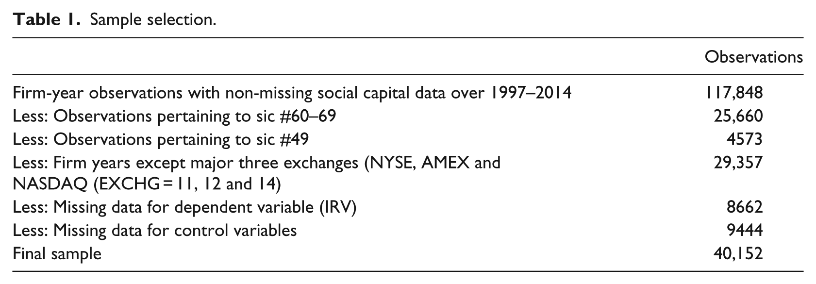
We collect data for this study from several sources: financial information from the Compustat annual database, stock returns and prices data from the Centre for Research in Security Prices (CRSP), daily factor data (e.g. SMB, HML and UMD) from the Kenneth R. French web site,¹ social capital data from the Northeast Regional Centre for Rural Development (NRCRD) at the Pennsylvania State University and finally, demographic data from the US Census Bureau and US Bureau of Economic Analysis (BEA). We use the state and county name of each firm’s headquarters’ location to match Compustat data with social capital data from the NRCRD. Our sample begins with 117,104 firm-year observations with available social capital data for the 1997–2014 sample period. We begin our sample period in 1997 because the new dataset on social capital became available from that point onward.² We then exclude firm-year observations from the financial industries (SIC 6000–6999) and regulated industries (SIC 4900–4949). This eliminates 30,233 firm-year observations. We exclude 29,357 firm-year observations pertaining to firms traded outside NYSE, AMEX and NASDAQ (EXCHG = 11, 12 and 14). Missing data for calculating the dependent variable (IRV) and the control variables reduce the sample to 40,152 firm-year observations. To avoid the undesirable influence of outliers, we winsorize the key variables in the extreme 1% of the respective distributions. Table 1 presents the sample selection. Variable definitions are presented in Appendix 1.

Table 1.

Sample selection.

	Observations
Firm-year observations with non-missing social capital data over 1997–2014	117,848
Less: Observations pertaining to sic #60–69	25,660
Less: Observations pertaining to sic #49	4573
Less: Firm years except major three exchanges (NYSE, AMEX and NASDAQ (EXCHG = 11, 12 and 14)	29,357
Less: Missing data for dependent variable (IRV)	8662
Less: Missing data for control variables	9444
Final sample	40,152

3.2. Empirical model

We estimate the following regression equation to test H1

\begin{matrix} I R V_{i, t} = γ_{0} + γ_{1} S C_{i, t} + γ_{2} S I Z E_{i, t} + γ_{3} L E V_{i, t} + γ_{4} M T B_{i, t} + γ_{5} R O A_{i, t} + γ_{6} D I V_{i, t} \\ + γ_{7} S T D_C F_{i, t} + γ_{8} H I N D E X_{i, t} + γ_{9} A G E_{i, t} + γ_{10} R E T_{i, t} + γ_{11} F R Q_{i, t} \\ + γ_{12} I N C O M E_{i, t} + γ_{13} E D U_{i, t} + γ_{14} % Δ P O P_{i, t} + \sum γ_{t} Y E A R_{t} + \sum γ_{t} I N D_{t} + ε_{i, t} \dots \end{matrix}

(1)

where the dependent variable, IRV, is estimated using a market model, capital asset pricing model (CAPM) and Fama–French (1993) model. The main independent variable is social capital (SC), which follows the social capital index developed by Rupasingha and Goetz (2008). We include a set of control variables that prior studies find to be associated with IRV. Large firms tend to diversify their businesses more efficiently and are less prone to bankruptcy. Therefore, these firms experience lower return volatility (Pastor and Veronesi, 2003). Hence, we control for firm size (SIZE) in the regression model. Rajgopal and Venkatachalam (2011) suggest that leverage (LEV) increases stockholders’ risk associated with the firm’s cash flow, suggesting a positive relationship between stock return volatility and financial leverage. Cao et al. (2008) show that firms with more growth opportunities are likely to experience higher IRV. We control for firm growth by using the market-to-book (MTB) ratio. Prior studies (e.g. Brown and Kapadia, 2007; Pastor and Veronesi, 2003; Wei and Zhang, 2006) argue that high profitability and stock return, and lower volatility in profit can enhance companies’ ability to lower financial instability and thus lessen idiosyncratic risk. Therefore, in the regression models, we control for firm profitability (ROA), stock return (RET), dividend payout (DIV) and cash flow risk (STD_CF).

Irvine and Pontiff (2009) suggest that competition among firms has important implications for idiosyncratic risk in terms of increasing cash flow variability. Therefore, we control for market competition using the Herfindahl index (HINDEX). Cao et al. (2008) argue that future cash flows of younger firms are more uncertain than those of older firms, indicating that firm age (AGE) affects firm-specific volatility. Rajgopal and Venkatachalam (2011) show that FRQ is associated with IRV. We estimate FRQ using the model developed by Kothari et al. (2005).³

We also include some county-level control variables to reduce the omitted variables problem. Recent research on the effects of social capital on different outcome variables follows this procedure (Hasan et al., 2017a, 2017b; Jha and Cox, 2015). INCOME is the natural log of median household income per capita in a county in a given year. EDU is the percentage of persons 25 years and over with at least 1 year of college in a county in a given year. Finally, ∆POP is the percentage of the population growth of the county since the previous year.⁴

To examine the moderating role of FRQ on the association between social capital and IRV (test of H2A), we develop the following model

\begin{matrix} I R V_{i, t} = γ_{0} + γ_{1} S C_{i, t} + γ_{2} F R Q_{i, t} + γ_{3} S C_{i, t} * F R Q_{i, t} + γ_{4} S I Z E_{i, t} + γ_{5} L E V_{i, t} + γ_{6} M T B_{i, t} \\ + γ_{7} R O A_{i, t} + γ_{8} D I V_{i, t} + γ_{9} S T D_C F_{i, t} + γ_{10} H I N D E X_{i, t} + γ_{11} A G E_{i, t} + γ_{12} R E T_{i, t} \\ + γ_{13} I N C O M E_{i, t} + γ_{14} E D U_{i, t} + γ_{15} % Δ P O P_{i, t} + \sum γ_{t} Y E A R_{t} + \sum γ_{t} I N D_{t} + ε_{i, t} \dots \end{matrix}

(2)

We expect the coefficient for SC*FRQ to be negative and significant to suggest that social capital, in concert with lower information asymmetry (proxied by FRQ), reduces the IRV of firms headquartered in high social capital regions.⁵

Finally, the following model is used to test the moderating role of CSR on the association between social capital and IRV (test of H2B)

\begin{matrix} I R V_{i, t} = γ_{0} + γ_{1} S C_{i, t} + γ_{2} C S R_{i, t} + γ_{3} S C_{i, t} * C S R_{i, t} + γ_{4} S I Z E_{i, t} + γ_{5} L E V_{i, t} \\ + γ_{6} M T B_{i, t} + γ_{7} R O A_{i, t} + γ_{8} D I V_{i, t} + γ_{9} S T D_C F_{i, t} + γ_{10} H I N D E X_{i, t} \\ + γ_{11} A G E_{i, t} + γ_{12} R E T_{i, t} + γ_{13} F R Q_{i, t} + γ_{14} I N C O M E_{i, t} + γ_{15} E D U_{i, t} \\ + γ_{16} % Δ P O P_{i, t} + \sum γ_{t} Y E A R_{t} + \sum γ_{t} I N D_{t} + ε_{i, t} \dots \end{matrix}

(3)

where CSR is the net CSR score estimated as the total strengths minus total concerns of CSR dimensions (Hasan and Habib, 2017a). Other variables are previously defined. We expect the coefficients for SC*CSR to be negative and significant to suggest that social capital, in concert with high CSR, reduces the IRV of firms headquartered in high social capital counties.

In order to isolate the direct and indirect effect (through FRQ) of social capital on IRV, we specify the following empirical model

I R V_{i, t} = γ_{0} + γ_{1} F R Q_{i, t} + γ_{2} S C_{i, t} + \sum_{j = 3}^{m} γ_{j} C o n t r o l s_{i, t} + \sum γ_{t} Y E A R_{t} + \sum γ_{t} I N D_{t} + ε_{i, t}

(4)

F R Q_{i, t} = α_{0} + α_{1} S C_{i, t} + \sum_{j = 3}^{n} α_{j} C o n t r o l s_{i, t} + \sum α_{t} Y E A R_{t} + \sum α_{t} I N D_{t} + ε_{i, t}

(5)

The model consists of two equations. Equation (4) exhibits how the FRQ channel influences IRV. The presence of SC in equation (4) allows for the possibility that SC may have a direct effect on IRV. Equation (5) shows how SC affects IRV through the FRQ channel (indirect effect). The controls for equation (4) are explained in Section 3.2. In equation (5), we control for SIZE, LEV, MTB, ROA, AGE, STD_CF, LOSS, Big4, ANALYST, %∆SALES, and year (YEAR) and industry (IND) fixed effects.

Furthermore, we specify the following empirical model to isolate the indirect effect of CSR on the association between social capital and IRV

I R V_{i, t} = γ_{0} + γ_{1} C S R_{i, t} + γ_{2} S C_{i, t} + \sum_{j = 3}^{m} γ_{j} C o n t r o l s_{i, t} + \sum γ_{t} Y E A R_{t} + \sum γ_{t} I N D_{t} + ε_{i, t}

(6)

C S R_{i, t} = α_{0} + α_{1} S C_{i, t} + \sum_{j = 3}^{n} α_{j} C o n t r o l s_{i, t} + \sum γ_{t} Y E A R_{t} + \sum γ_{t} I N D_{t} + ε_{i, t}

(7)

The empirical process for the CSR channel is same as outlined for the FRQ channel. In equation (7), we control for SIZE, LEV, MTB, ROA, AGE, STD_CF, CASH_RATIO, R&D and YEAR and IND fixed effects.⁶

For the above estimation, we use the Maximum Likelihood (ML) method as a simultaneous equations model which allows for correlations between the error terms across equations (Cheung, 2016). The direct effect of SC on IRV is $γ_{2}$ , while the indirect effect is $γ_{1} α_{1}$ for the FRQ and CSR channels in equations (4) and (6), respectively.

3.3. Dependent variable: IRV

We use daily stock returns as a basis of calculating annual estimates of IRV. In doing so, we run the following market model, CAPM and Fama–French (1993) three-factor regressions for each firm in each year. We require at least 175 daily observations to compute IRV.

3.3.1. Market model

R_{i, t} = α_{i} + β_{i} (R_{m, t}) + ε_{i, t}, i = 1, \dots, N a n d t = 1, \dots, T

(8)

where R_i,t is the raw stock return on day t for firm i, R_m,t is the daily return from the CRSP value-weighted market index, α_i (or alpha) is the intercept term, β_i (or beta) is the slope coefficient that captures systematic risk and ε_i,t is an error term. The standard deviation of the residuals from the above regression model is our annual measure of IRV.

3.3.2. CAPM model

R_{i, t} - R_{f, t} = α_{i} + β_{i} (R_{m, t} - R_{f, t}) + ε_{i, t}, i = 1, \dots, N a n d t = 1, \dots, T

(9)

where R_i,t is the stock return on day t for firm i, R_f,t is the simple daily return from holding a 30-day risk-free treasury bill and the remaining variables are as in equation (8).

3.3.3. Fama–French (1993) model

R_{i, t} - R_{f, t} = α_{i} + β_{i} (R_{m, t} - R_{f, t}) + γ_{i} S M B_{t} + ϕ_{i} H M L_{t} + ε_{i, t}, i = 1, \dots, N a n d t = 1, \dots, T

(10)

where SMB_t and HML_t are the size premium (small minus big) and the value premium (high minus low) respectively, collected from Kenneth French’s web site, and the remaining variables are as in equation (8).

3.4. Independent variable (social capital)

Following Rupasingha and Goetz (2008), we construct a county-level index to measure social capital. As in their study, we use two measures of norms and two measures of networks. The two measures of norms are the census-mail response rate and the votes cast in presidential elections. The two measures of networks are the number of associations and non-profit organizations each per 10,000 people. Using these four indicators, we conduct a principal component analysis for each year (1997, 2005 and 2009). We use the first component for each year and consider it the social capital index. We linearly interpolate the data to fill in the years 1998–2004, 2006–2008 and 2010–2014, as in Hasan et al. (2017a and 2017b) and Jha and Cox (2015).

4. Descriptive statistics

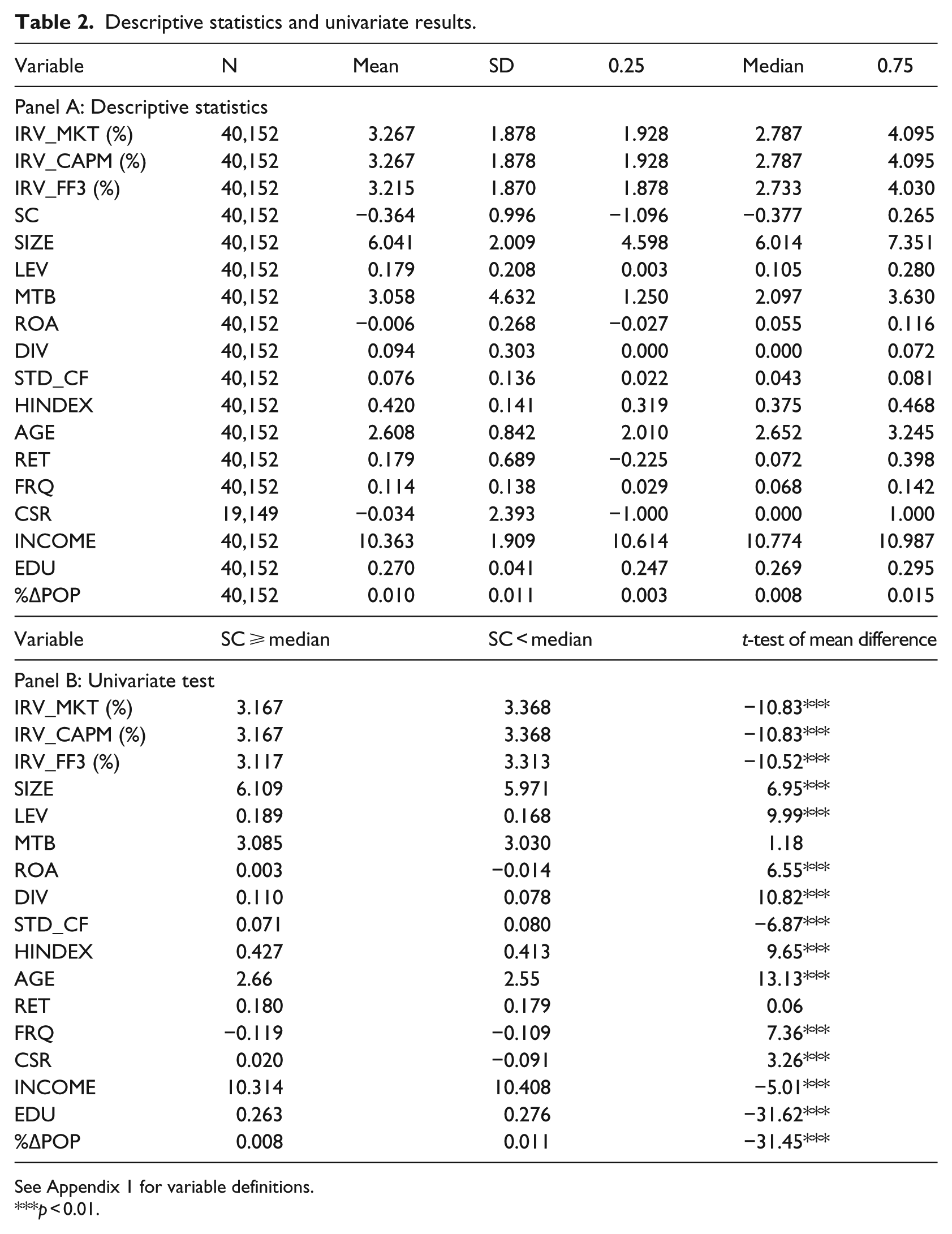
Panel A of Table 2 presents the descriptive statistics for the key variables used in the regression models. Results indicate that the annual estimates of mean (median) IRV based on the market and CAPM models are 3.27% (2.79%), whereas the IRV measure based on the Fama–French three-factor model is 3.22% (2.73%). The mean (median) value of SC is −0.36 (−0.38). The standard deviation of SC is 0.996 and the corresponding interquartile spread ranges from −1.10 to 0.27, indicating considerable variation in the levels of social capital. Sample firms, on average, are growth firms (an average MB ratio of 3.06) with negative profitability (mean ROA is −0.60%), low payout ratio (mean DIV is 9.4%) and low leverage (mean LEV is 17.9%).

Table 2.

Descriptive statistics and univariate results.

Variable	N	Mean	SD	0.25	Median	0.75
Panel A: Descriptive statistics
IRV_MKT (%)	40,152	3.267	1.878	1.928	2.787	4.095
IRV_CAPM (%)	40,152	3.267	1.878	1.928	2.787	4.095
IRV_FF3 (%)	40,152	3.215	1.870	1.878	2.733	4.030
SC	40,152	−0.364	0.996	−1.096	−0.377	0.265
SIZE	40,152	6.041	2.009	4.598	6.014	7.351
LEV	40,152	0.179	0.208	0.003	0.105	0.280
MTB	40,152	3.058	4.632	1.250	2.097	3.630
ROA	40,152	−0.006	0.268	−0.027	0.055	0.116
DIV	40,152	0.094	0.303	0.000	0.000	0.072
STD_CF	40,152	0.076	0.136	0.022	0.043	0.081
HINDEX	40,152	0.420	0.141	0.319	0.375	0.468
AGE	40,152	2.608	0.842	2.010	2.652	3.245
RET	40,152	0.179	0.689	−0.225	0.072	0.398
FRQ	40,152	0.114	0.138	0.029	0.068	0.142
CSR	19,149	−0.034	2.393	−1.000	0.000	1.000
INCOME	40,152	10.363	1.909	10.614	10.774	10.987
EDU	40,152	0.270	0.041	0.247	0.269	0.295
%∆POP	40,152	0.010	0.011	0.003	0.008	0.015
Variable	SC ⩾ median		SC < median		t-test of mean difference
Panel B: Univariate test
IRV_MKT (%)	3.167		3.368		−10.83***
IRV_CAPM (%)	3.167		3.368		−10.83***
IRV_FF3 (%)	3.117		3.313		−10.52***
SIZE	6.109		5.971		6.95***
LEV	0.189		0.168		9.99***
MTB	3.085		3.030		1.18
ROA	0.003		−0.014		6.55***
DIV	0.110		0.078		10.82***
STD_CF	0.071		0.080		−6.87***
HINDEX	0.427		0.413		9.65***
AGE	2.66		2.55		13.13***
RET	0.180		0.179		0.06
FRQ	−0.119		−0.109		7.36***
CSR	0.020		−0.091		3.26***
INCOME	10.314		10.408		−5.01***
EDU	0.263		0.276		−31.62***
%∆POP	0.008		0.011		−31.45***

See Appendix 1 for variable definitions.

***

p < 0.01.

Panel B of Table 2 presents the mean difference test of variables between high and low SC counties. Our results show that the mean IRV (e.g. IRV_MKT and IRV_CAPM) for firms in high SC counties is 3.17%, but it is 3.37% in the low SC counties. A two-tailed t-test (p-value) for the difference between the two groups is −10.83 (< 0.001), suggesting that the IRVs of firms headquartered in high SC counties are significantly lower than firms headquartered in low SC counties. Firms in high SC counties are significantly larger, older, more levered, more profitable and pay more dividends. Moreover, firms headquartered in high SC counties are less risky and characterized by better FRQ.

Table 3 presents the correlation analysis. The correlation between IRV and SC is negative and significant at p < 0.001 (correlation of −0.06) supporting H1. With respect to the correlation among IRV and other control variables, we find that larger, older, profitable firms and firms with more dividends and better FRQ are negatively correlated with IRV, while firms with more leverage and volatile cash flows are positively correlated with IRV.

Table 3.

Correlation analysis.

	IRV_MKT	SC	SIZE	LEV	MTB	ROA	DIV	CFO	HINDEX	AGE	RET	FRQ	INCOME	EDU	%∆POP
IRV_MKT
SC	−0.058	–
SIZE	−0.592	0.032	–
LEV	0.089	0.043	−0.105	–
MTB	−0.034	0.008	0.204	−0.203	–
ROA	−0.452	0.031	0.321	−0.021	−0.009	–
DIV	−0.215	0.048	0.158	0.032	0.015	0.122	–
STD_CF	0.294	−0.040	−0.211	−0.143	0.088	−0.395	−0.083	–
HINDEX	−0.097	0.040	0.018	0.047	−0.030	0.085	0.047	−0.062	–
AGE	−0.348	0.080	0.256	0.062	−0.054	0.216	0.142	−0.222	0.161	–
RET	0.020	−0.009	0.077	−0.104	0.155	0.117	−0.014	−0.014	0.003	−0.002	–
FRQ	−0.265	0.035	0.155	0.134	−0.114	0.265	0.091	−0.270	0.064	0.188	−0.048	–
INCOME	0.105	−0.029	−0.031	0.030	−0.001	−0.038	−0.003	0.029	0.001	−0.016	−0.003	0.005	–
EDU	−0.018	−0.114	−0.036	0.028	−0.025	0.011	0.025	−0.009	0.060	0.009	0.009	−0.015	−0.018	–
%∆POP	0.031	−0.218	0.015	0.045	0.002	0.015	−0.013	−0.004	−0.028	−0.077	0.004	0.009	0.015	0.205	−

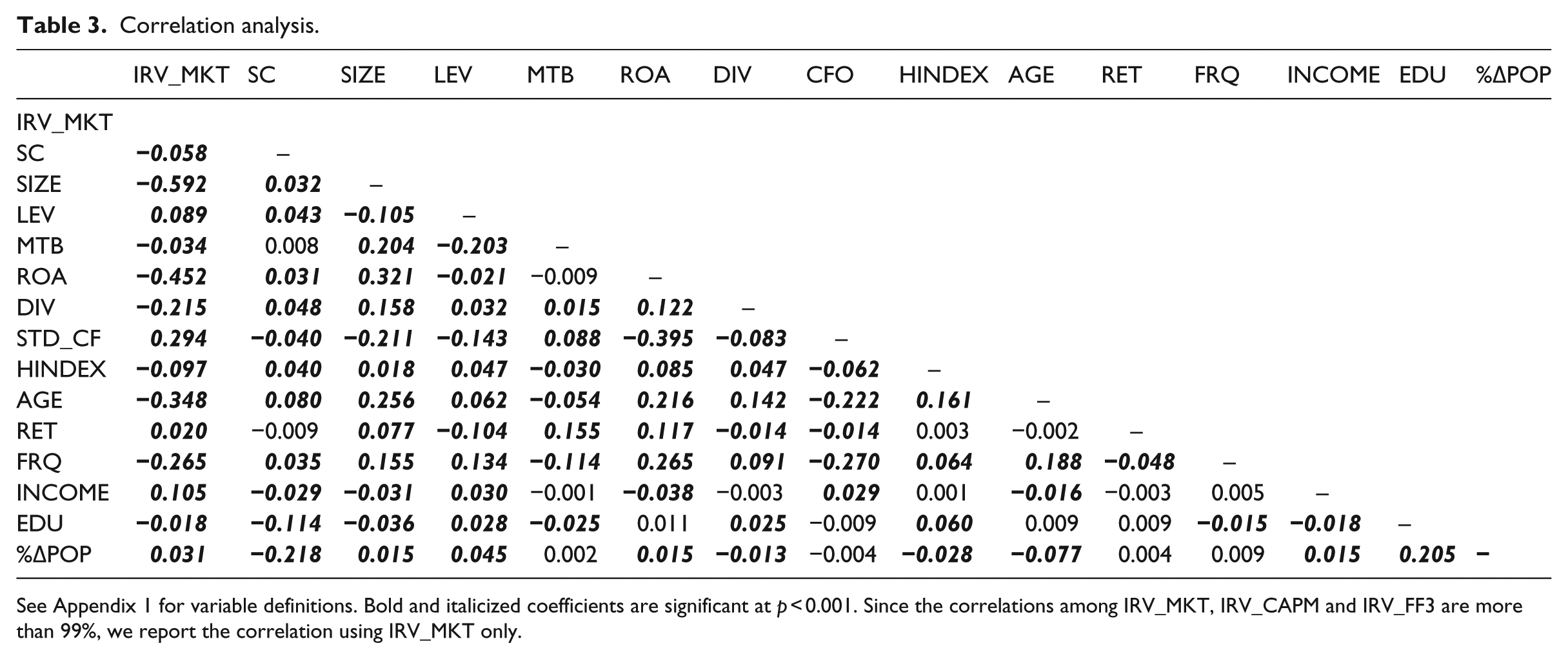
See Appendix 1 for variable definitions. Bold and italicized coefficients are significant at p < 0.001. Since the correlations among IRV_MKT, IRV_CAPM and IRV_FF3 are more than 99%, we report the correlation using IRV_MKT only.

5. Relationship between social capital and IRV

5.1. Baseline multiple regression results

Table 4 presents the baseline regression results of the association between SC and IRV. We estimate the regression models using ordinary least squares (OLS) regressions with standard errors adjusted for heteroscedasticity and within-firm clustering.⁷ In Table 4, across all models, the dependent variable is IRV, the test variable is SC and regression models include firm-level and county-level controls, with dummies to control for industry and year fixed effects. The estimates for SC across all models are negative and significant. In particular, the coefficients in columns (1), (2) and (3) are −0.028 (p < 0.01), −0.028 (p < 0.01) and −0.026 (p < 0.05), respectively.⁸ These results suggest that firms headquartered in US counties with higher levels of SC are associated with significantly lower IRV after controlling for firm and county characteristics, lending support to our H1.⁹ The effect of SC on IRV is economically meaningful as well. In Model 1, for example, an increase in social capital from the 25th percentile to 75th percentile would reduce the IRV by 0.038 ( = −0.028 × 1.361, where −0.028 is the coefficient estimate in column (1) of Table 4, and 1.361 is the interquartile range of SC calculated from descriptive statistics reported in Panel A of Table 2. The reported coefficients in column (1) also suggests that a firm that is headquartered in a county in the 75th percentile of the SC is associated with a 24% lower IRV compared to a firm headquartered in a county in the 25th percentile of SC ((−0.028*0.265)/( −0.028*−1.096)).

Table 4.

Social capital and idiosyncratic return volatility: Baseline regressions.

Variables	(1)	(2)	(3)
Variables	IRV_MKT	IRV_CAPM	IRV_FF3
Constant	4.642*** [18.92]	4.642*** [18.92]	4.659*** [18.91]
SC	−0.028*** [−2.64]	−0.028*** [−2.64]	−0.026** [−2.43]
SIZE	−0.382*** [−47.49]	−0.382*** [−47.49]	−0.389*** [−47.60]
LEV	0.678*** [10.15]	0.678*** [10.15]	0.672*** [10.07]
MTB	0.015*** [7.31]	0.015*** [7.31]	0.015*** [7.30]
ROA	−1.603*** [−33.11]	−1.603*** [−33.11]	−1.590*** [−32.87]
DIV	−0.401*** [−15.75]	−0.401*** [−15.75]	−0.393*** [−15.43]
STD_CF	0.698*** [7.35]	0.698*** [7.35]	0.702*** [7.42]
HINDEX	0.035 [0.30]	0.035 [0.30]	0.039 [0.34]
AGE	−0.235*** [−16.19]	−0.235*** [−16.19]	−0.230*** [−15.86]
RET	0.264*** [20.24]	0.264*** [20.24]	0.268*** [20.72]
FRQ	−1.079*** [17.96]	−1.079*** [17.96]	−1.064*** [17.71]
INCOME	0.028*** [7.12]	0.028*** [7.12]	0.027*** [6.86]
EDU	−0.029 [−0.10]	−0.029 [−0.10]	−0.087 [−0.29]
%∆POP	0.716 [0.75]	0.716 [0.75]	0.775 [0.82]
YEAR FE	YES	YES	YES
INDUSTRY FE	YES	YES	YES
Adj. R²	0.60	0.60	0.60
Observations	40,152	40,152	40,152
No. of firms	4,056	4,056	4,056

See Appendix 1 for variable definitions. Robust t-statistics in brackets.

***

p < 0.01; **p < 0.05.

The regression results in Table 4 show that the coefficients of most of the control variables have the predicted signs and statistical significance. For example, in accordance with the empirical findings (e.g. Brown and Kapadia, 2007; Chen et al., 2012; Ferreira and Laux, 2007; Rajgopal and Venkatachalam, 2011), we find that large (SIZE), profitable (ROA) and mature (AGE) firms and firms with better FRQ are associated with a lower level of IRV, but growth (MTB) and leveraged firms (LEV), and firms with volatile cash flows (STD_CF), are associated with a higher level of IRV. Moreover, the positive coefficient of RET is consistent with the findings of Brown and Kapadia (2007).

5.2. Sensitivity tests

5.2.1. Alternative measure of social capital

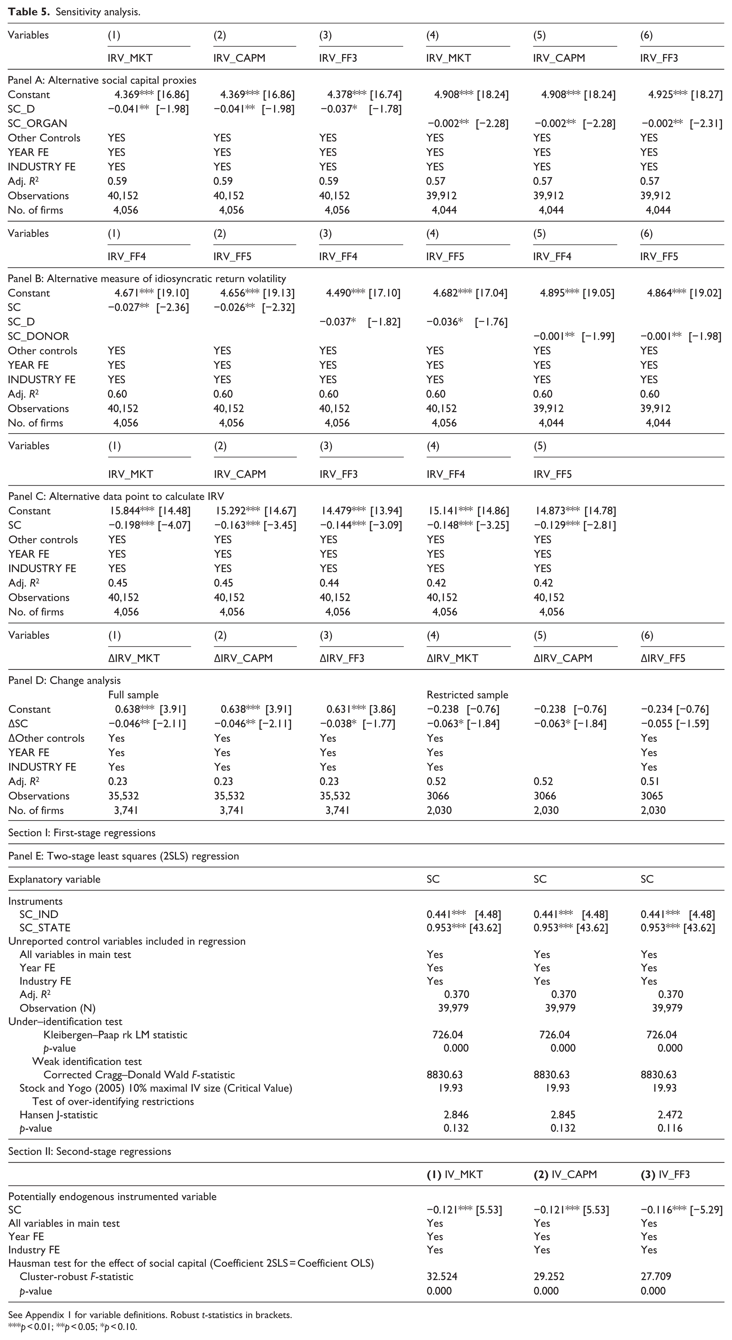
To allay concerns that our results might be biased because of measurement error associated with the calculation of social capital index, we follow Jha and Cox (2015) and use a dichotomous measure of social capital instead of a continuous variable. We create an indicator variable, SC_D, that takes a value of 1 if the firm is headquartered in a county with more than the median level of social capital, and 0 otherwise. Regression results reported in columns (1)–(3) in Panel A of Table 5 are consistent with those in the baseline regression; the coefficient of SC_D is both negative and significant.

Table 5.

Sensitivity analysis.

Variables	(1)	(2)	(3)	(4)	(5)	(6)
Variables	IRV_MKT	IRV_CAPM	IRV_FF3	IRV_MKT	IRV_CAPM	IRV_FF3
Panel A: Alternative social capital proxies
Constant	4.369*** [16.86]	4.369*** [16.86]	4.378*** [16.74]	4.908*** [18.24]	4.908*** [18.24]	4.925*** [18.27]
SC_D	−0.041** [−1.98]	−0.041** [−1.98]	−0.037* [−1.78]
SC_ORGAN				−0.002** [−2.28]	−0.002** [−2.28]	−0.002** [−2.31]
Other Controls	YES	YES	YES	YES	YES	YES
YEAR FE	YES	YES	YES	YES	YES	YES
INDUSTRY FE	YES	YES	YES	YES	YES	YES
Adj. R²	0.59	0.59	0.59	0.57	0.57	0.57
Observations	40,152	40,152	40,152	39,912	39,912	39,912
No. of firms	4,056	4,056	4,056	4,044	4,044	4,044
Variables	(1)	(2)	(3)	(4)	(5)	(6)
Variables	IRV_FF4	IRV_FF5	IRV_FF4	IRV_FF5	IRV_FF4	IRV_FF5
Panel B: Alternative measure of idiosyncratic return volatility
Constant	4.671*** [19.10]	4.656*** [19.13]	4.490*** [17.10]	4.682*** [17.04]	4.895*** [19.05]	4.864*** [19.02]
SC	−0.027** [−2.36]	−0.026** [−2.32]
SC_D			−0.037* [−1.82]	−0.036* [−1.76]
SC_DONOR					−0.001** [−1.99]	−0.001** [−1.98]
Other controls	YES	YES	YES	YES	YES	YES
YEAR FE	YES	YES	YES	YES	YES	YES
INDUSTRY FE	YES	YES	YES	YES	YES	YES
Adj. R²	0.60	0.60	0.60	0.60	0.60	0.60
Observations	40,152	40,152	40,152	40,152	39,912	39,912
No. of firms	4,056	4,056	4,056	4,056	4,044	4,044
Variables	(1)	(2)	(3)	(4)	(5)
Variables	IRV_MKT	IRV_CAPM	IRV_FF3	IRV_FF4	IRV_FF5
Panel C: Alternative data point to calculate IRV
Constant	15.844*** [14.48]	15.292*** [14.67]	14.479*** [13.94]	15.141*** [14.86]	14.873*** [14.78]
SC	−0.198*** [−4.07]	−0.163*** [−3.45]	−0.144*** [−3.09]	−0.148*** [−3.25]	−0.129*** [−2.81]
Other controls	YES	YES	YES	YES	YES
YEAR FE	YES	YES	YES	YES	YES
INDUSTRY FE	YES	YES	YES	YES	YES
Adj. R²	0.45	0.45	0.44	0.42	0.42
Observations	40,152	40,152	40,152	40,152	40,152
No. of firms	4,056	4,056	4,056	4,056	4,056
Variables	(1)	(2)	(3)	(4)	(5)	(6)
Variables	ΔIRV_MKT	ΔIRV_CAPM	ΔIRV_FF3	ΔIRV_MKT	ΔIRV_CAPM	ΔIRV_FF5
Panel D: Change analysis
	Full sample			Restricted sample
Constant	0.638*** [3.91]	0.638*** [3.91]	0.631*** [3.86]	−0.238 [−0.76]	−0.238 [−0.76]	−0.234 [−0.76]
ΔSC	−0.046** [−2.11]	−0.046** [−2.11]	−0.038* [−1.77]	−0.063* [−1.84]	−0.063* [−1.84]	−0.055 [−1.59]
ΔOther controls	Yes	Yes	Yes	Yes		Yes
YEAR FE	Yes	Yes	Yes	Yes		Yes
INDUSTRY FE	Yes	Yes	Yes	Yes		Yes
Adj. R²	0.23	0.23	0.23	0.52	0.52	0.51
Observations	35,532	35,532	35,532	3066	3066	3065
No. of firms	3,741	3,741	3,741	2,030	2,030	2,030
Section I: First-stage regressions
Panel E: Two-stage least squares (2SLS) regression
Explanatory variable				SC	SC	SC
Instruments
SC_IND				0.441*** [4.48]	0.441*** [4.48]	0.441*** [4.48]
SC_STATE				0.953*** [43.62]	0.953*** [43.62]	0.953*** [43.62]
Unreported control variables included in regression
All variables in main test				Yes	Yes	Yes
Year FE				Yes	Yes	Yes
Industry FE				Yes	Yes	Yes
Adj. R²				0.370	0.370	0.370
Observation (N)				39,979	39,979	39,979
Under–identification test
Kleibergen–Paap rk LM statistic				726.04	726.04	726.04
p-value				0.000	0.000	0.000
Weak identification test
Corrected Cragg–Donald Wald F-statistic				8830.63	8830.63	8830.63
Stock and Yogo (2005) 10% maximal IV size (Critical Value)				19.93	19.93	19.93
Test of over-identifying restrictions
Hansen J-statistic				2.846	2.845	2.472
p-value				0.132	0.132	0.116
Section II: Second-stage regressions
				(1) IV_MKT	(2) IV_CAPM	(3) IV_FF3
Potentially endogenous instrumented variable
SC				−0.121*** [5.53]	−0.121*** [5.53]	−0.116*** [−5.29]
All variables in main test				Yes	Yes	Yes
Year FE				Yes	Yes	Yes
Industry FE				Yes	Yes	Yes
Hausman test for the effect of social capital (Coefficient 2SLS = Coefficient OLS)
Cluster-robust F-statistic				32.524	29.252	27.709
p-value				0.000	0.000	0.000

See Appendix 1 for variable definitions. Robust t-statistics in brackets.

***

p < 0.01; **p < 0.05; *p < 0.10.

Prior studies (e.g. Buonanno et al., 2009; Guiso et al., 2004; Hasan et al., 2017a,b) also use blood and organ donation as an alternate proxy for social capital. Following these studies, we use the organ donation data from the Organ Procurement and Transplantation Network (OPTN) to construct an alternative measure of social capital (SC_ORGAN). Columns (4)–(6) in Panel A of Table 5 show that the coefficient of SC_ORGAN, the alternative proxy for social capital, is negative (β₁ = –0.002) and significant (p < 0.05 or better), suggesting that our finding is robust to the alternative measure of social capital.

5.2.2. Alternative measure of IRV

In our main analysis, we use three measures of IRV: the market model, CAPM and Fama–French three-factor model. In this section, we re-estimate our analysis using the three-factor Fama–French (1993) model, including a momentum factor as in Carhart (1997) and Fama–French (2016) four-factor models. Panel B of Table 5 shows that regression results using IRV_FF4 and IRV_FF5, alternative estimates of IRV, corroborate the conclusions from our main analyses. In particular, we continue to find a negative and statistically significant coefficient for all variants of SC, suggesting that the specific measure of IRV does not drive our main finding.

As a further robustness check, we use monthly stock returns instead of daily returns to construct the IRV. Results reported in Panel C of Table 5 are largely consistent with the results reported in the main analysis. In particular, coefficients for SC are all negative and significant (p < 0.01), indicating the robustness of the reported results. Our inference from analysis remains robust even if we use 5-year rolling IRV estimated from monthly stock returns (results unreported).

5.2.3. Omitted variable bias

It is possible that our analysis omits some other determinants of IRV from the regressions that are correlated with other included variables. Xu and Malkiel (2003) show that the proportion of institutional ownership is correlated with firm-specific risk. Prior studies (Luo and Bhattacharya, 2009; Mishra and Modi, 2013) show that CSR is associated with IRV. To mitigate potential problems arising from correlated omitted variables, we re-estimate the regression incorporating institutional shareholding and net CSR. Data requirements for these additional control variables reduce the sample size to around 18,000 firm-year observations. Despite the reduction in sample size, the coefficient of untabulated results shows that the association between SC and IRV remains qualitatively similar in terms of sign, significance and magnitude, suggesting that our reported results are unlikely to be driven by omitted correlated time-invariant variables.

5.2.4. Change analysis

Although our analysis controls for a variety of firm characteristics that might account for the association between social capital and IRV, there might still be concern over the use of a mostly time-invariant proxy of social capital. One way to address this potential concern is to conduct a ‘change’ analysis. We argue that if social capital drives the decrease in IRV, then the change in social capital should have a first-order effect on changes in IRV. Therefore, we modify the ‘levels’ specification in equation (1) to a ‘change’ specification, wherein we regress annual changes in IRV on changes in social capital along with changes in other economic determinants. Reported results in Panel D of Table 5 (columns 1–3) show a negative and significant association between changes in SC index and changes in IRV over time. For example, the coefficient in columns (1) and (2) is −0.046 (both p < 0.05). In addition to annual change analysis, we also conduct a change specification between 1997 and 2005, and between 2005 and 2009. This restricted change analysis alleviates any concern over the use of interpolated data in this study. Reported results (columns 4–6) largely corroborate the findings in the main analysis. Interestingly, the coefficients in change analysis are relatively large, even though the statistical significance is relatively moderate. Overall, we are able to document that firms headquartered in a high social capital counties are associated with less IRV.

5.2.5. Fama–MacBeth regression

One may argue that SC is largely time-invariant and most of the variation in this variable is cross-sectional instead of time-series. Therefore, as a robustness test, we rerun the regressions using the Fama and MacBeth (1973) cross-sectional regression method. Untabulated results show that the coefficient for the baseline SC variable is −0.040 (p < 0.01) for IRV_MKT and IRV_CAPM, and −0.037 (p < 0.01) for IRV_FF3. These results are consistent with our main regression results reported in Table 4. Furthermore, our results remain robust even when we re-estimate equation (1) with time-level cluster (i.e. cluster by year).

5.2.6. Is the association between social capital and IRV driven by an endogeneity problem?

Our analysis so far suggests that social capital reduces firms’ IRV. However, the sign, magnitude and statistical significance of these estimates may be biased if social capital is correlated with the error term (ε). We use an instrumental variable technique to validate our interpretation of the results documented in Table 4. This should also alleviate any concerns over reverse causality or omitted variable bias in the OLS (Wooldridge, 2010). Motivated by Jha and Cox (2015), we use (1) the industry-level mean social capital in each year, where an industry is defined by its two-digit SIC code and (2) the state-level mean social capital in each year. The spatially sticky nature of social capital (Rutten et al., 2010) makes industry and state-level social capital suitable instruments. Prior studies (Baptista and Swann, 1998) show that industries tend to cluster in certain geographic areas. It follows that the social capital of firms in an industry might be similar (Jha and Cox, 2015). Moreover, it is reasonable to expect that state-level social capital is highly correlated with the social capital of the counties located in that particular state. Therefore, we expect both industry and state-level social capital to be highly and positively correlated with our endogenous variable, social capital. It is highly unlikely that IRV affects the industry and state-level social capital. It is also unlikely that the industry and state-level social capital affects IRV other than through the social capital of the firm where it is headquartered; thus, the essential requirements of the instruments are satisfied.

Panel E of Table 5 (Section 1) reports that coefficients on the instrumental variables are positive and significant (p < 0.001), suggesting that the included industry and state-level SC are significantly associated with the county-level SC. Results in Section 2 suggest that the relationship between social capital and IRV remains robust after accounting for the endogenous relationship between social capital and IRV. For example, the estimated coefficients (and p values) of social capital are −0.121 (p < 0.01), −0.121 (p < 0.01) and −0.116 (p < 0.01) for the IRV_MKT, IRV_CAPM and IRV_FF3 measures of IRV. Overall, results using 2SLS suggest that endogeneity cannot explain away the documented negative relationship between the social capital and IRV.

In Panel E of Table 5, under-identification test results (LM statistic) reveal that the excluded instruments are ‘relevant’ because the Kleibergen–Paap rk LM statistic is significant at p < 0.001. The weak instrument test results show that the excluded instruments are correlated with the endogenous regressors, because the Cragg–Donald Wald F statistic (8830.63) is greater than the Stock and Yogo (2005) critical value (i.e. 19.93) at 10%. Results from Hansen’s over-identifying restrictions test do not reject the null hypothesis (p > 0.10), suggesting that the instruments are uncorrelated with the error term and are correctly excluded from the second stage regression, which reflects the validity of the instruments used for the 2SLS regression. Finally, the Hausman (1978) test significantly rejects (p < 0.001) the exogeneity of the social capital, justifying the use of the 2SLS regression estimates. Overall, this result corroborates our primary findings that social capital reduces the IRV of the firm.

5.3. Empirical analysis of the FRQ and CSR channels (test of H2)

5.3.1. Social capital, FRQ and IRV: Interaction results

Extant studies document that better FRQ reduces IRV (Chen et al., 2012; Rajgopal and Venkatachalam, 2011). Recent empirical evidence suggests that firms headquartered in high social capital regions are associated with better FRQ (Jha, 2017). Our main regression results also indicate a significant negative association between social capital and IRV. Since firms from high social capital regions are associated with better FRQ (and lower IRV), and FRQ reduces IRV, it follows that SC, when interacted with FRQ, should have a more profound effect on reducing IRV. To test this assertion, we add the term SC×FRQ to our baseline model. We present the results of this analysis in columns (1), (2) and (3) of Table 6 (Panel A). We estimate FRQ using the model developed by Kothari et al. (2005) and multiply the absolute value of FRQ by −1, so that higher values indicate better FRQ. We find the coefficient for FRQ to be negative and significant (coefficient −1.085 in columns (1) and (2) and −1.065 in column (3), both significant at p < 0.01), suggesting that FRQ reduces the IRV. We continue to find negative and significant coefficients for SC. Our variable of primary interest is the interactive coefficient SC × FRQ. We find a significantly (p < 0.01) negative coefficient for the interaction variable (coefficient −1.017 in columns (1) and (2) and −1.023 for column (3)). These results indicate that the effect of social capital in reducing IRV is more pronounced in the presence of FRQ. In particular, the role of SC in reducing IRV is expected to accentuate from 0.111 to −0.004 when FRQ moves from the first to the third quartile. For brevity, we present only the coefficients of the key independent variables in the Table.

Table 6.

Interaction results.

Variables	IRV_MKT	IRV_CAPM	IRV_FF3
Panel A: Social capital, FRQ and IRV
Constant	4.732*** [19.20]	4.732*** [19.20]	4.747*** [19.19]
SC	−0.033*** [−2.83]	−0.033*** [−2.83]	−0.030*** [−2.61]
FRQ	−1.085*** [−17.78]	−1.085*** [−17.78]	−1.065*** [−17.58]
SC ×FRQ	−1.017*** [−3.23]	−1.017*** [−3.23]	−1.023*** [−3.21]
Other Controls	Yes	Yes	Yes
YEAR FE	Yes	Yes	Yes
INDUSTRY FE	Yes	Yes	Yes
Adj. R²	0.60	0.60	0.60
Observations	40,152	40,152	40,152
No. of firms	4,056	4,056	4,056
Variables	IRV_MKT	IRV_CAPM	IRV_FF3
Panel B: Social capital, CSR and IRV
Constant	4.141*** [21.37]	4.141*** [21.37]	4.085*** [21.60]
SC	−0.033*** [−3.07]	−0.033*** [−3.07]	−0.031*** [−2.89]
CSR	0.014*** [3.52]	0.014*** [3.52]	0.016*** [3.91]
SC ×CSR	−0.094*** [−3.64]	−0.094*** [−3.64]	−0.116*** [−4.54]
Other Controls	Yes	Yes	Yes
YEAR FE	Yes	Yes	Yes
INDUSTRY FE	Yes	Yes	Yes
Adj. R-squared	0.54	0.54	0.53
Observations	19,149	19,149	19,149
No. of firms	2,696	2,696	2,696

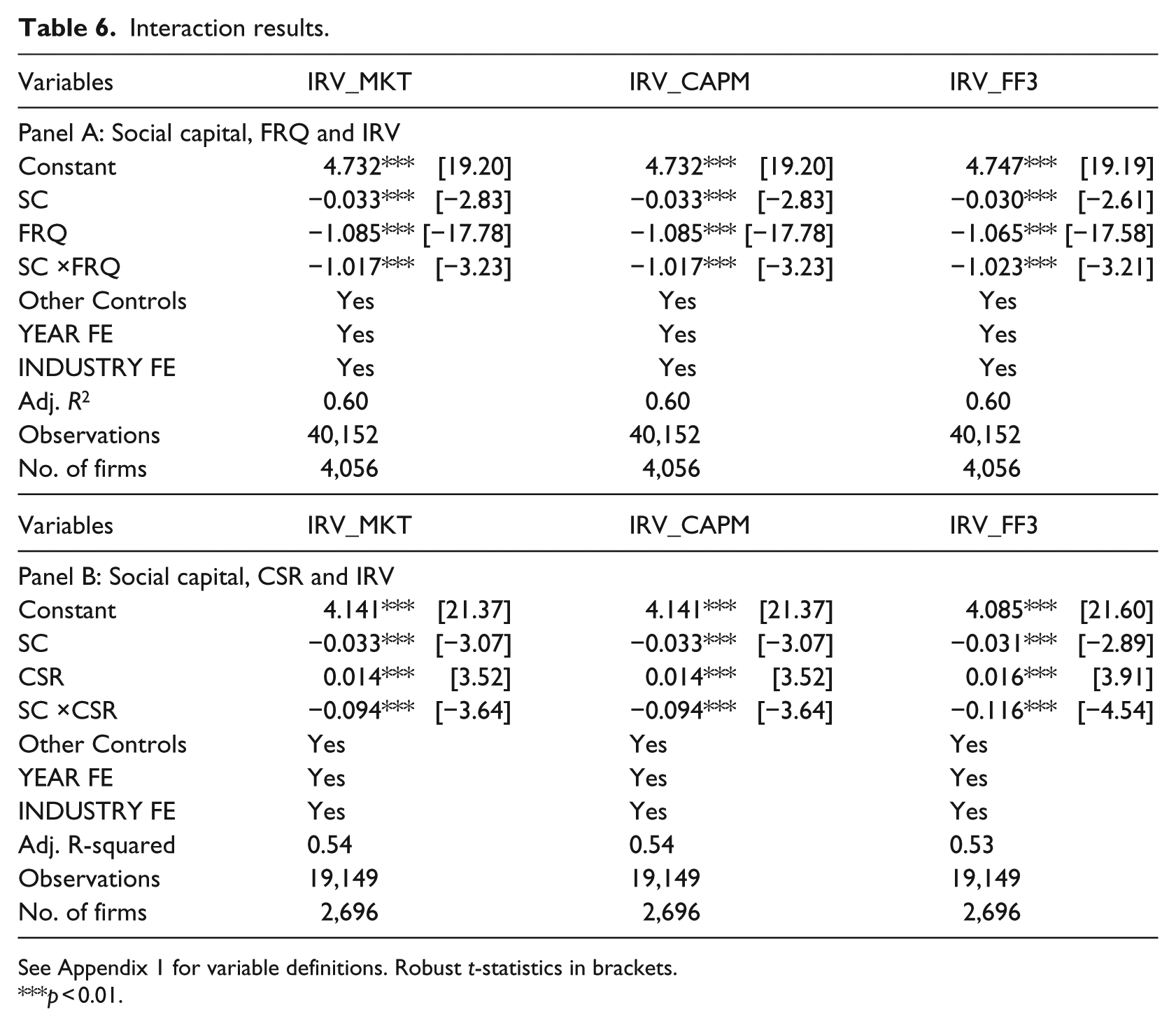
See Appendix 1 for variable definitions. Robust t-statistics in brackets.

***

p < 0.01.

5.3.2. Social capital, CSR and IRV: Interaction results

Extant studies provide evidence that CSR lowers undesirable firm-idiosyncratic risk (Luo and Bhattacharya, 2009; Mishra and Modi, 2013). In a recent study, Jha and Cox (2015) show that firms headquartered in high social capital regions exhibit higher CSR. To test whether CSR, when interacted with social capital, has any incremental effect on reducing IRV, we include CSR and the interaction term SC × CSR in our baseline model and report the results in Panel B of Table 6. We continue to find negative and significant coefficients for SC. Coefficients for CSR are positive and significant. Interestingly, we find a significantly (p < 0.01) negative coefficient for the interaction variable (SC × CSR), implying that in the presence of CSR, SC reduces IRV. In particular, the role of SC in IRV accentuates from 0.061 to −0.127 when CSR moves from the first to the third quartile.

5.4. Distinguishing the direct and indirect effects of social capital

Table 4 suggests that social capital has additional explanatory power in reducing IRV, even after explicitly controlling for known firm-specific variables, county-level demographic variables, and industry and year fixed effects. A related issue is the extent to which social capital affects IRV directly (without mediation by any other variable in the model) and indirectly through its effect on firms’ FRQ or CSR activities, the so-called mediation effect. We use simultaneous equation models to define and estimate such effects. In our settings, direct effects are effects from social capital to IRV (SC→IRV) that are not mediated by any other variable in the model. Indirect effects are paths from social capital to IRV that travel through at least one other variable (FRQ or CSR). The sum of direct and indirect effects represents the total effect.

Panel A of Table 7 tests FRQ as a channel and Panel B tests CSR as another channel. Results reported in Panel A show that the effect of SC and FRQ on IRV is negative and significant, suggesting that SC and FRQ directly (i.e. independently) reduce IRV (direct effect, without the inclusion of the mediator). Furthermore, SC, through its effect on firms’ FRQ (indirect effect), reduces IRV, but this effect is statistically insignificant. However, the total effect of SC on IRV is negative (coefficients of −0.024 for IRV_MKT and IRV_CAPM, and −0.017 for IRV_FF3) and statistically significant (p < 0.01). Panel A also indicates that the proportion of total effect that is mediated is less than 20%. The coefficient of determination suggests that the models explain more than 64% of the variation. The Sobel test (p < 0.01) also signifies the partial mediation effect.

Table 7.

Direct and indirect effects of social capital.

Variables	IRV_MKT	FRQ	IRV_CAPM	FRQ	IRV_FF3	FRQ
Panel A: FRQ as the channel
I. Maximum likelihood (ML) estimation results
Constant	2.448*** [9.37]	0.181*** [10.16]	2.448*** [9.37]	0.181*** [10.16]	2.481*** [9.52]	0.182*** [10.16]
FRQ	−8.50*** [11.32]	–	−8.50*** [11.32]	–	−8.298*** [10.98]	–
SC	−0.020** [2.21]	0.0005 [0.61]	−0.020** [2.16]	0.0005 [0.61]	−0.017** [−1.96]	0.0005 [0.61]
All Other Controls	Yes	Yes	Yes	Yes	Yes	Yes
Industry and Year Dummies	Yes	Yes	Yes	Yes	Yes	Yes
Log pseudolikelihood	1911842.4	–	1911842.4	–	1910952.6	–
Observations	31,470	31,470	1,470	31,470	31,470	31,470
Coefficient of Determination	0.64	0.64	0.64	0.64	0.64	0.64
Sobel Z	−0.017***	−0.017***	−0.017***	−0.017***	−0.017***	−0.017***
p–value of Sobel Z	0.000	0.000	0.000	0.000	0.000	0.000
II. Direct, indirect and total effect of social capital
	IRV_MKT		IRV_CAPM		IRV_FF3
Direct effect
SC	−0.020** [2.21]		−0.020** [2.16]		−0.017** [−1.96]
Indirect effect – through FRQ
SC	−0.004 [−0.61]		−0.004 [−0.61]		−0.004 [−0.63]
Total effect
SC	−0.024*** [−3.34]		−0.024*** [−3.16]		−0.021*** [−2.93]
Proportion of total effect that is mediated	16.67%		16.67%		19.05%
Indirect to direct effect	20.00%		20.00%		23.53%
Variables	IRV_MKT	CSR	IRV_CAPM	CSR	IRV_FF3	CSR
Panel B: CSR as the channel
I. Maximum likelihood (ML) estimation results
Constant	3.029*** [15.77]	−3.002*** [6.15]	3.029*** [15.76]	−3.002*** [6.15]	2.989*** [15.84]	−3.002*** [6.15]
CSR	−0.114*** [2.98]	–	−0.114*** [2.98]	–	−0.110*** [2.85]	–
SC	−0.025*** [−3.37]	0.050*** [2.82]	−0.025*** [−3.25]	0.050*** [2.82]	−0.023* [−1.88]	0.050*** [2.82]
All Other Controls	Yes	Yes	Yes	Yes	Yes	Yes
Industry and Year Dummies	Yes	Yes	Yes	Yes	Yes	Yes
Log pseudolikelihood	1281066.7	–	1281066.7	–	1281310.4	–
Observations	19,149	19,149	19,149	19,149	19,149	19,149
Coefficient of Determination	0.57	0.57	0.57	0.57	0.57	0.57
Sobel Z	−0.006***	−0.006***	−0.006***	−0.006***	−0.006***	−0.006***
p–value of Sobel Z	0.000	0.000	0.000	0.000	0.000	0.000
II. Direct, indirect and total effect of social capital
	IRV_MKT		IRV_CAPM		IRV_FF3
Direct effect
SC	−0.025*** [−3.37]		−0.025*** [−3.25]		−0.023* [−1.88]
Indirect effect – through CSR
SC	−0.006** [−2.11]		−0.006** [−1.98]		−0.006** [−2.00]
Total effect
SC	−0.031*** [−4.27]		−0.031*** [−3.08]		−0.029** [−2.48]
Proportion of total effect that is mediated	19.35%		19.35%		20.69%
Indirect to direct effect	24.00%		24.00%		26.09%

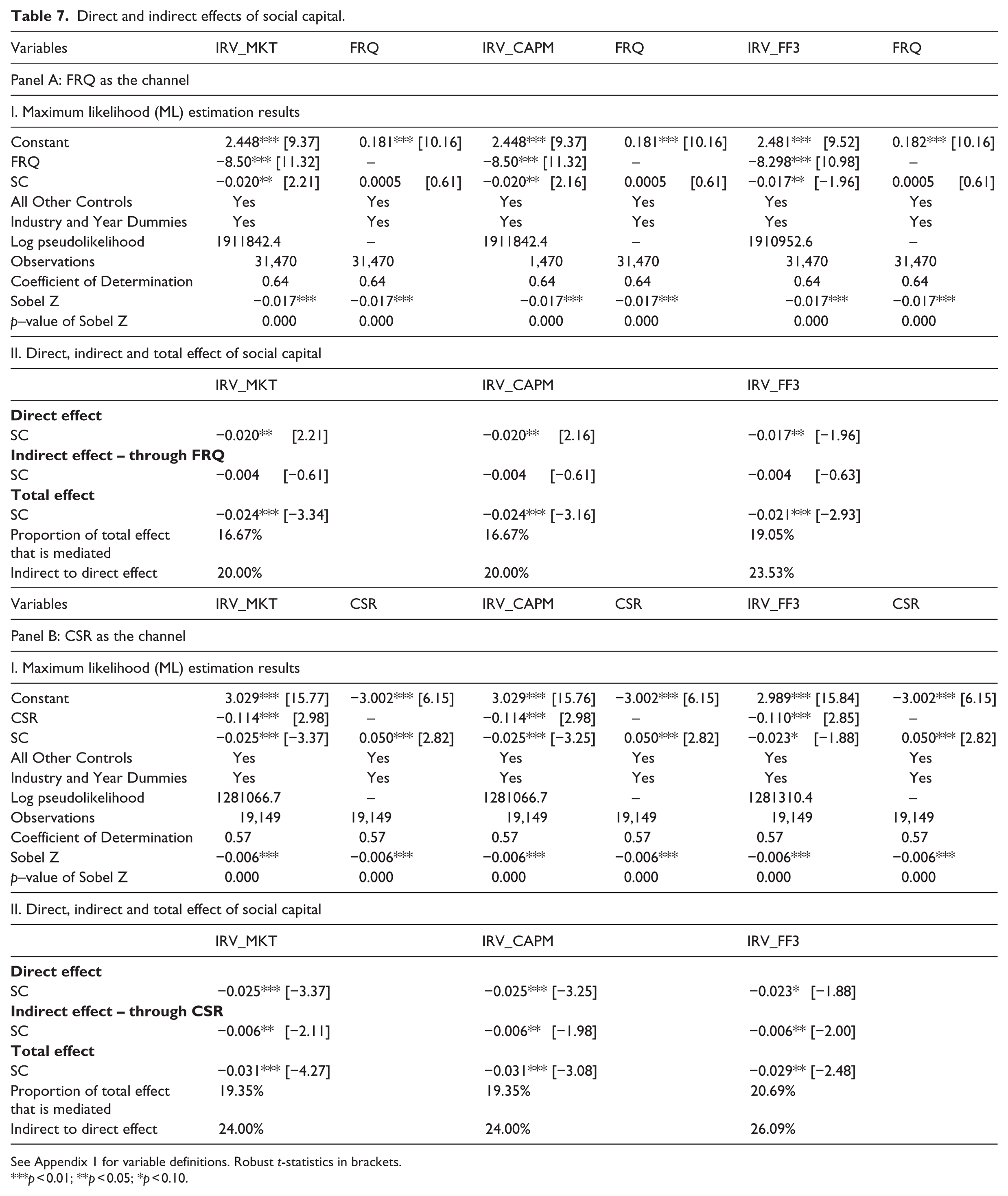
See Appendix 1 for variable definitions. Robust t-statistics in brackets.

***

p < 0.01; **p < 0.05; *p < 0.10.

Panel B shows that the direct and indirect effects of SC (through CSR) on IRV are negative and significant (p < 0.01), suggesting that SC, both individually and through CSR, reduces IRV. The total effect of SC (sum of direct and indirect effects) on IRV is negative (coefficients of −0.031 for IRV_MKT and IRV_CAPM, and −0.029 for IRV_FF3) and significant (p < 0.01). Results indicate that the proportion of the total effect that is mediated is around 20%. The coefficient of determination (57%) indicates the goodness of fit of the model, and the Sobel test (p < 0.01) suggests the significance of the mediation effect (CSR). Overall, these results signify that social capital, both individually and collectively (though FRQ and CSR channels), reduces firm-level IRV, lending support to our hypotheses.

5.5. Additional analysis: Social capital, geographic dispersion of firms and IRV

Our key argument is that prevalent social capital favourably affects the informational environment and CSR: hence, firms headquartered in a high social capital county are associated with less IRV. If this is the case, then we should expect the relationship between social capital and IRV to be more pronounced for firms that are less geographically dispersed. As is consistent with Jha and Cox (2015), we emphasize that social norms of less geographically dispersed firms are likely to be largely congruent with the norms of the managers, and therefore, the social capital’s effect is much more salient. Following Jha and Cox (2015), we split the sample firms by the median level of subsidiaries, which is six in our case. Results reported in columns (1) and (2) of Table 8 show that the effect of social capital on IRV is much stronger (−0.042) and statistically significant (p < 0.01) for less geographically dispersed firms. However, the effect of social capital on IRV is much weaker (−0.019) and statistically insignificant (p > 0.10) for more geographically dispersed firms. We continue to find similar results when we split the sample by the mean number of subsidiaries (five). An F-test suggests that the difference between high and low subsidiaries is significant at 5%. We obtain qualitatively similar results with alternative measure of IRV (results untabulated).

Table 8.

Social capital, geographic dispersion and IRV.

Dept. Var. = IRV_MKT	(Model 1)	(Model 2)	(Model 3)	(Model 4)
Dept. Var. = IRV_MKT	No. of subsidiaries ⩾6	No. of subsidiaries < 6	No. of subsidiaries ⩾5	No. of subsidiaries < 5
Constant	3.837*** [9.82]	5.135*** [18.76]	3.826*** [9.84]	5.199*** [18.75]
SC	−0.019 [−1.46]	−0.042*** [−2.89]	−0.019 [−1.48]	−0.042*** [−2.86]
SIZE	−0.280*** [−23.41]	−0.432*** [−41.67]	−0.284*** [−24.29]	−0.436*** [−41.18]
LEV	0.686*** [6.52]	0.686*** [8.67]	0.685*** [6.70]	0.693*** [8.62]
MTB	0.016*** [5.89]	0.013*** [5.38]	0.018*** [6.56]	0.012*** [4.94]
ROA	−1.604*** [−17.07]	−1.573*** [−28.46]	−1.602*** [−17.92]	−1.571*** [−27.81]
DIV	−0.314*** [−11.32]	−0.440*** [−13.27]	−0.317*** [−11.64]	−0.438*** [−12.99]
STD_CF	1.208*** [4.95]	0.568*** [5.79]	1.313*** [5.29]	0.539*** [5.53]
HINDEX	0.021 [0.15]	0.065 [0.44]	0.039 [0.27]	0.045 [0.30]
AGE	−0.223*** [−11.56]	−0.283*** [−15.55]	−0.223*** [−11.85]	−0.288*** [−15.46]
RET	0.120*** [4.37]	0.303*** [20.38]	0.122*** [4.67]	0.307*** [20.42]
FRQ	1.319*** [11.90]	0.989*** [14.26]	1.235*** [11.53]	1.001*** [14.11]
INCOME	0.029*** [5.40]	0.027*** [5.58]	0.028*** [5.34]	0.027*** [5.37]
EDU	0.057 [0.15]	0.005 [0.01]	0.087 [0.23]	−0.22 [−0.06]
%∆POP	0.331 [0.25]	1.031 [0.88]	0.222 [0.18]	1.087 [0.92]
Diff in Coeff. of SC
p -value		0.026		0.034
YEAR FE	YES	YES	YES	YES
INDUSTRY FE	YES	YES	YES	YES
Adj. R²	0.59	0.57	0.58	0.57
Observations	13,176	29,676	14,244	25,908
No. of firms	2,578	3,400	2,657	3,341

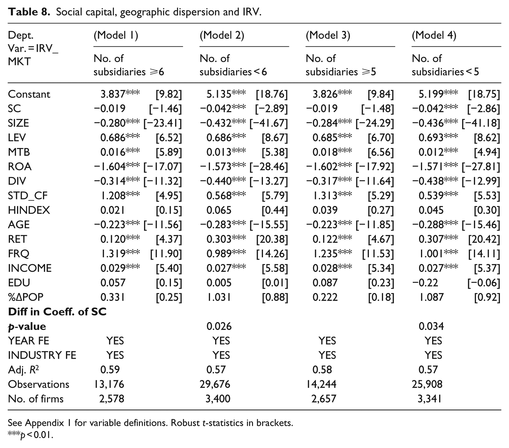
See Appendix 1 for variable definitions. Robust t-statistics in brackets.

***

p < 0.01.

6. Conclusion

In this study, we explore the association between the social capital of US counties and the IRV of the firms. We argue that the prevalent social capital favourably affects the informational environment and CSR, reducing uncertainty about future cash flows and associated IRV. As is consistent with our expectation, we find that firms headquartered in US counties with higher social capital are associated with significantly lower levels of IRV than are firms from low social capital regions. Through a range of sensitivity analyses, we establish that the effect of social capital on IRV is robust. Additional analysis shows that the association between social capital and IRV is moderated by FRQ and CSR. When we estimate the direct and indirect effects of social capital on IRV, we find that the direct effect of social capital captures around 80% of the total effect. Finally, we find that the effect of social capital on IRV is more pronounced for less geographically dispersed firms.

Our results contribute to an emerging stream of literature that examines the influence of social capital on corporate economic behaviour. To date, very few studies have examined the effect of social influences on publicly listed corporations, with the notable exceptions of Hasan et al. (2017a,b), Jha and Chen (2015) and Jha and Cox (2015). We bring together the two disparate streams of literature on social capital and IRV and thereby contribute to this nascent literature.

Footnotes

Appendix

Appendix 1.

Variable definitions.

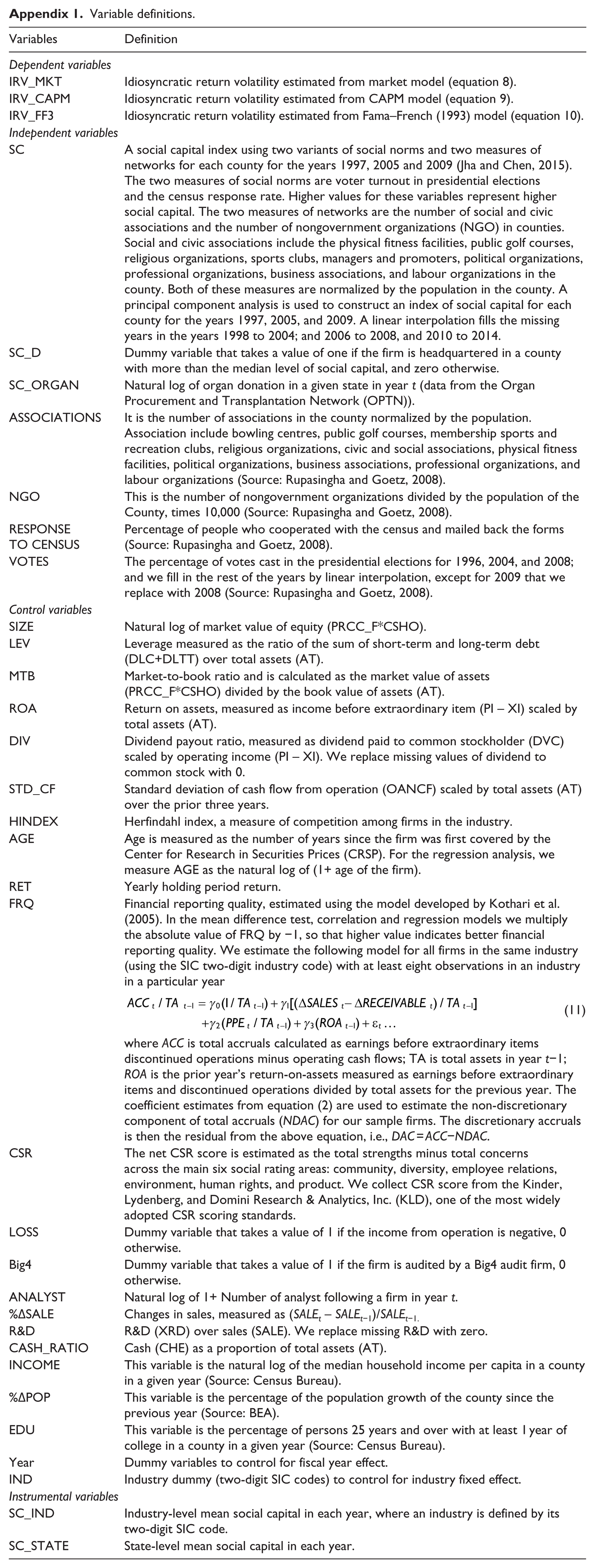
Variables	Definition
Dependent variables
IRV_MKT	Idiosyncratic return volatility estimated from market model (equation 8).
IRV_CAPM	Idiosyncratic return volatility estimated from CAPM model (equation 9).
IRV_FF3	Idiosyncratic return volatility estimated from Fama–French (1993) model (equation 10).
Independent variables
SC	A social capital index using two variants of social norms and two measures of networks for each county for the years 1997, 2005 and 2009 (Jha and Chen, 2015). The two measures of social norms are voter turnout in presidential elections and the census response rate. Higher values for these variables represent higher social capital. The two measures of networks are the number of social and civic associations and the number of nongovernment organizations (NGO) in counties. Social and civic associations include the physical fitness facilities, public golf courses, religious organizations, sports clubs, managers and promoters, political organizations, professional organizations, business associations, and labour organizations in the county. Both of these measures are normalized by the population in the county. A principal component analysis is used to construct an index of social capital for each county for the years 1997, 2005, and 2009. A linear interpolation fills the missing years in the years 1998 to 2004; and 2006 to 2008, and 2010 to 2014.
SC_D	Dummy variable that takes a value of one if the firm is headquartered in a county with more than the median level of social capital, and zero otherwise.
SC_ORGAN	Natural log of organ donation in a given state in year t (data from the Organ Procurement and Transplantation Network (OPTN)).
ASSOCIATIONS	It is the number of associations in the county normalized by the population. Association include bowling centres, public golf courses, membership sports and recreation clubs, religious organizations, civic and social associations, physical fitness facilities, political organizations, business associations, professional organizations, and labour organizations (Source: Rupasingha and Goetz, 2008).
NGO	This is the number of nongovernment organizations divided by the population of the County, times 10,000 (Source: Rupasingha and Goetz, 2008).
RESPONSE TO CENSUS	Percentage of people who cooperated with the census and mailed back the forms (Source: Rupasingha and Goetz, 2008).
VOTES	The percentage of votes cast in the presidential elections for 1996, 2004, and 2008; and we fill in the rest of the years by linear interpolation, except for 2009 that we replace with 2008 (Source: Rupasingha and Goetz, 2008).
Control variables
SIZE	Natural log of market value of equity (PRCC_F*CSHO).
LEV	Leverage measured as the ratio of the sum of short-term and long-term debt (DLC+DLTT) over total assets (AT).
MTB	Market-to-book ratio and is calculated as the market value of assets (PRCC_F*CSHO) divided by the book value of assets (AT).
ROA	Return on assets, measured as income before extraordinary item (PI – XI) scaled by total assets (AT).
DIV	Dividend payout ratio, measured as dividend paid to common stockholder (DVC) scaled by operating income (PI – XI). We replace missing values of dividend to common stock with 0.
STD_CF	Standard deviation of cash flow from operation (OANCF) scaled by total assets (AT) over the prior three years.
HINDEX	Herfindahl index, a measure of competition among firms in the industry.
AGE	Age is measured as the number of years since the firm was first covered by the Center for Research in Securities Prices (CRSP). For the regression analysis, we measure AGE as the natural log of (1+ age of the firm).
RET	Yearly holding period return.
FRQ	Financial reporting quality, estimated using the model developed by Kothari et al. (2005). In the mean difference test, correlation and regression models we multiply the absolute value of FRQ by −1, so that higher value indicates better financial reporting quality. We estimate the following model for all firms in the same industry (using the SIC two-digit industry code) with at least eight observations in an industry in a particular year (11) $\begin{matrix} A C C_{t} / T A_{t - 1} = γ_{0} (1 / T A_{t - 1}) + γ_{1} [(Δ S A L E S_{t} - Δ R E C E I V A B L E_{t}) / T A_{t - 1}] \\ + γ_{2} (P P E_{t} / T A_{t - 1}) + γ_{3} (R O A_{t - 1}) + ε_{t} \dots \end{matrix}$ where ACC is total accruals calculated as earnings before extraordinary items discontinued operations minus operating cash flows; TA is total assets in year t−1; ROA is the prior year’s return-on-assets measured as earnings before extraordinary items and discontinued operations divided by total assets for the previous year. The coefficient estimates from equation (2) are used to estimate the non-discretionary component of total accruals (NDAC) for our sample firms. The discretionary accruals is then the residual from the above equation, i.e., DAC = ACC−NDAC.
CSR	The net CSR score is estimated as the total strengths minus total concerns across the main six social rating areas: community, diversity, employee relations, environment, human rights, and product. We collect CSR score from the Kinder, Lydenberg, and Domini Research & Analytics, Inc. (KLD), one of the most widely adopted CSR scoring standards.
LOSS	Dummy variable that takes a value of 1 if the income from operation is negative, 0 otherwise.
Big4	Dummy variable that takes a value of 1 if the firm is audited by a Big4 audit firm, 0 otherwise.
ANALYST	Natural log of 1+ Number of analyst following a firm in year t.
%∆SALE	Changes in sales, measured as (SALE_t – SALE_t₋₁)/SALE_t_−1.
R&D	R&D (XRD) over sales (SALE). We replace missing R&D with zero.
CASH_RATIO	Cash (CHE) as a proportion of total assets (AT).
INCOME	This variable is the natural log of the median household income per capita in a county in a given year (Source: Census Bureau).
%∆POP	This variable is the percentage of the population growth of the county since the previous year (Source: BEA).
EDU	This variable is the percentage of persons 25 years and over with at least 1 year of college in a county in a given year (Source: Census Bureau).
Year	Dummy variables to control for fiscal year effect.
IND	Industry dummy (two-digit SIC codes) to control for industry fixed effect.
Instrumental variables
SC_IND	Industry-level mean social capital in each year, where an industry is defined by its two-digit SIC code.
SC_STATE	State-level mean social capital in each year.

Acknowledgements

We thank Karen Benson (Editor), Sue Wright (Associate Editor), and two anonymous referees for their valuable feedback and suggestions. We also thank Adrian Cheung and Robert Durand for many helpful comments.

Final transcript accepted 4 June 2017 by Sue Wright (AE Accounting).

Funding

The authors disclosed receipt of the following financial support for the research, authorship, and/or publication of this article: We gratefully acknowledge financial support from the School of Economics and Finance, Curtin Business School, Curtin University.

Notes

References

Aiken

West

(1991) Multiple Regression: Testing and Interpreting Interactions. Newbury Park, CA: SAGE.

Ang

Hodrick

Xing

et al . (2006) The cross section of volatility and expected returns. The Journal of Finance 61: 259–299.

Avramov

Chordia

Jostova

et al . (2013) Anomalies and financial distress. Journal of Financial Economics 108: 139–159.

Bali

Cakici

(2008) Idiosyncratic volatility and the cross section of expected returns. Journal of Financial and Quantitative Analysis 43: 29–58.

Bali

Cakici

Whitelaw

(2011) Maxing out: Stocks as lotteries and the cross-section of expected returns. Journal of Financial Economics 99: 427–446.

Bansal

Clelland

(2004) Talking trash: Legitimacy, impression management, and unsystematic risk in the context of the natural environment. Academy of Management Journal 47: 93–103.

Baptista

Swann

(1998) Do firms in clusters innovate more? Research Policy 27: 525–540.

Bauernschuster

Falck

Heblich

(2010) Social capital access and entrepreneurship. Journal of Economic Behavior & Organization 76: 821–833.

Bennett

Sias

Starks

(2003) Greener pastures and the impact of dynamic institutional preferences. Review of Financial Studies 16: 1203–1238.

10.

Boyer

Mitton

Vorkink

(2010) Expected idiosyncratic skewness. Review of Financial Studies 23: 169–202.

11.

Brown

Kapadia

(2007) Firm-specific risk and equity market development. Journal of Financial Economics 84: 358–388.

12.

Buonanno

Montolio

Vanin

(2009) Does social capital reduce crime? Journal of Law and Economics 52: 145–170.

13.

Campbell

Lettau

Malkiel

et al . (2001) Have individual stocks become more volatile? An empirical exploration of idiosyncratic risk. Journal of Finance 56: 1–43.

14.

Cao

Simin

Zhao

(2008) Can growth options explain the trend in idiosyncratic risk? Review of Financial Studies 21: 2599–2633.

15.

Carhart

(1997) On persistence in mutual fund performance. Journal of Finance 52: 57–82.

16.

Chen

Huang

Jha

(2012) Idiosyncratic return volatility and the information quality underlying managerial discretion. Journal of Financial and Quantitative Analysis 47: 873–899.

17.

Cheung

AWK

(2016) Corporate social responsibility and corporate cash holdings. Journal of Corporate Finance 37: 412–430.

18.

Clayton

Hartzell

Rosenberg

(2005) The impact of CEO turnover on equity volatility. Journal of Business 78: 1779–1808.

19.

Coleman

(1988) Social capital in the creation of human capital. American Journal of Sociology 94: S95–S120.

20.

Coleman

(1994) Foundations of Social Theory. Cambridge, MA: Harvard University Press.

21.

Dasgupta

Gan

Gao

(2010) Transparency, price informativeness, and stock return synchronicity: Theory and evidence. Journal of Financial and Quantitative Analysis 45: 1189–1220.

22.

Dechow

Sloan

Sweeney

(1995) Detecting earnings management. The Accounting Review 70: 193–225.

23.

Diamond

Verrecchia

(1991) Disclosure, liquidity, and the cost of capital. Journal of Finance 46: 1325–1359.

24.

Dorn

Huberman

(2005) Talk and action: What individual investors say and what they do. Review of Finance 9: 437–481.

25.

Easley

O’Hara

(2004) Information and the cost of capital. Journal of Finance 59: 1553–1583.

26.

Fama

French

(1993) Common risk factors in the returns on stocks and bonds. Journal of Financial Economics 33: 3–56.

27.

Fama

French

(2016) Dissecting anomalies with a five-factor model. Review of Financial Studies 29: 69–103.

28.

Fama

MacBeth

(1973) Risk, return, and equilibrium: Empirical tests. The Journal of Political Economy 81: 607–636.

29.

Ferreira

Laux

(2007) Corporate governance, idiosyncratic risk, and information flow. Journal of Finance 62: 951–989.

30.

Fombrun

(1996) Reputation. Hoboken, NJ: John Wiley & Sons.

31.

Fombrun

Gardberg

Barnett

(2000) Opportunity platforms and safety nets: Corporate citizenship and reputational risk. Business and Society Review 105: 85–106.

32.

Fox

Morck

Yeung

et al . (2003) Law, share price accuracy, and economic performance: The new evidence. Michigan Law Review 103: 331–386.

33.

Freeman

(1984) Stakeholder Management: Framework and Philosophy. Mansfield, MA: Pitman Publishing.

34.

Froot

Scharfstein

Stein

(1992) Herd on the street: Informational inefficiencies in a market with short-term speculation. Journal of Finance 47: 1461–1484.

35.

Fukuyama

(1997) Social capital and the modern capitalist economy: Creating a high trust workplace. Stern Business Magazine 4: 1–16.

36.

Fukuyama

(2001) Social capital, civil society and development. Third World Quarterly 22: 7–20.

37.

Goetzmann

Kumar

(2008) Equity portfolio diversification. Review of Finance 12: 433–463.

38.

Goyal

Santa-Clara

(2003) Idiosyncratic risk matters! Journal of Finance 58: 975–1008.

39.

Gruca

Rego

(2005) Customer satisfaction, cash flow, and shareholder value. Journal of Marketing 69: 1–130.

40.

Guiso

Sapienza

Zingales

(2004) The role of social capital in financial development. American Economic Review 94: 526–556.

41.

Guo

Savickas

(2008) Average idiosyncratic volatility in G7 countries. Review of Financial Studies 21: 1259–1296.

42.

Han

Kumar

(2013) Speculative retail trading and asset prices. Journal of Financial and Quantitative Analysis 48: 377–404.

43.

Hasan

Hoi

CKS

(2017b) Does social capital matter in corporate decisions? Evidence from corporate tax avoidance. Journal of Accounting Research 55: 629–658.

44.

Hasan

Hoi

CKS

Zhang

(2017a) Social capital and debt contracting: Evidence from bank loans and public bonds. Journal of Financial and Quantitative Analysis 52: 1017–1047.

45.

Hasan

Habib

(2017a) Corporate life cycle, organizational financial resources and corporate social responsibility. Journal of Contemporary Accounting and Economics 13: 20–36.

46.

Hasan

Habib

(2017b) Firm life cycle and idiosyncratic volatility. International Review of Financial Analysis 50: 164–175.

47.

Hausman

(1978) Specification tests in econometrics. Econometrica 46: 1251–1271.

48.

Healy

Hutton

Palepu

(1999) Stock performance and intermediation changes surrounding sustained increases in disclosure. Contemporary Accounting Research 16: 485–520.

49.

Hillman

Keim

(2001) Shareholder value, stakeholder management, and social issues: What’s the bottom line? Strategic Management Journal 22: 125–139.

50.

Hou

Loh

(2016) Have we solved the idiosyncratic volatility puzzle? Journal of Financial Economics 121: 167–194.

51.

Irvine

Pontiff

(2009) Idiosyncratic return volatility, cash flows, and product market competition. Review of Financial Studies 22: 1149–1177.

52.

Jha

(2017) Financial reports and social capital. Journal of Business Ethics. Epub ahead of print 14 March 2017. DOI: 10.1007/s10551-017-3495-5.

53.

Jha

Cox

(2015) Corporate social responsibility and social capital. Journal of Banking and Finance 60: 252–270.

54.

Jha

Chen

(2015) Audit fees and social capital. Accounting Review 90: 611–639.

55.

Jiang

Yao

(2009) The information content of idiosyncratic volatility. Journal of Financial and Quantitative Analysis 44: 1–28.

56.

Johnson

(2004) Forecast dispersion and the cross section of expected returns. The Journal of Finance 59: 1957–1978.

57.

Kothari

Leone

Wasley

(2005) Performance matched discretionary accrual measures. Journal of Accounting and Economics 39: 163–197.

58.

LaPorta

Lopez-De-Silanes

Shleifer

Vishny

(1997) Trust in large organizations. American Economic Review 87: 333–338.

59.

Leung

Srinidhi

Lobo

(2012) Family control and idiosyncratic volatility: Evidence from listed firms in Hong Kong. Journal of Contemporary Accounting and Economics 8: 39–52.

60.

Leuz

Verrecchia

(2000) The economic consequences of increased disclosure. Journal of Accounting Research 38: 91–124.

61.

Liu

Di lorio

(2016) The pricing of idiosyncratic volatility: An Australian study. Australian Journal of Management 41: 353–375.

62.

Lui

Markov

Tamayo

(2007) What makes a stock risky? Evidence from sell-side analysts’ risk ratings. Journal of Accounting Research 45: 629–665.

63.

Luo

Bhattacharya

(2006) Corporate social responsibility, customer satisfaction, and market value. Journal of Marketing 70: 1–18.

64.

Luo

Bhattacharya

(2009) The debate over doing good: Corporate social performance, strategic marketing levers, and firm-idiosyncratic risk. Journal of Marketing 73: 198–213.

65.

McAlister

Srinivasan

Kim

(2007) Advertising, research and development, and systematic risk of the firm. Journal of Marketing 71: 35–48.

66.

March

Shapira

(1987) Managerial perspectives on risk and risk taking. Management Science 33: 1404–1418.

67.

Merton

(1987) A simple model of capital market equilibrium with incomplete information. The Journal of Finance 42: 483–510.

68.

Milgram

Bickman

Berkowitz

(1969) Note on the drawing power of crowds of different size. Journal of Personality and Social Psychology 13: 79–82.

69.

Mishra

Modi

(2013) Positive and negative corporate social responsibility, financial leverage, and idiosyncratic risk. Journal of Business Ethics 117: 431–448.

70.

Morck

Yeung

(2013) R-squared and the Economy. Working paper no. w19017, 7 June. Cambridge, MA: National Bureau of Economic Research.

71.

Mueller

(2011) Returns to private equity-idiosyncratic risk does matter! Review of Finance 15: 545–574.

72.

Nartea

Ward

Yao

(2011) Idiosyncratic volatility and cross-sectional stock returns in Southeast Asian stock markets. Accounting & Finance 51: 1031–1054.

73.

O’Hara

(2003) Presidential address: liquidity and price discovery. Journal of Finance 58: 1335–1354.

74.

Pastor

Veronesi

(2003) Stock valuation and learning about profitability. Journal of Finance 58: 1749–1789.

75.

Pevzner

Xie

Xin

(2015) When firms talk, do investors listen? The role of trust in stock market reactions to corporate earnings announcements. Journal of Financial Economics 117: 190–223.

76.

Pontiff

(2006) Costly arbitrage and the myth of idiosyncratic risk. Journal of Accounting and Economics 42: 35–52.

77.

Rajgopal

Venkatachalam

(2011) Financial reporting quality and idiosyncratic return volatility. Journal of Accounting and Economics 51: 1–20.

78.

Rupasingha

Goetz

(2008) US County-Level Social Capital Data, 1990–2005. University Park, PA: The Northeast Regional Center for Rural Development, Penn State University.

79.

Rutten

Westlund

Boekema

(2010) The spatial dimension of social capital. European Planning Studies 18: 863–871.

80.

Sault

(2005) Movements in Australian stock volatility: A disaggregated approach. Australian Journal of Management 30: 303–320.

81.

Sharpe

(1964) Capital asset prices: A theory of market equilibrium under conditions of risk. The Journal of Finance 19: 425–442.

82.

Spagnolo

(1999) Social relations and cooperation in organizations. Journal of Economic Behavior & Organization 38: 1–25.

83.

Stock

Yogo

(2005) Testing for weak instruments in linear IV regression. In: Andrews

EWK

(ed.) Identification and Inference for Econometric Models: Essays in Honor of Thomas Rothenberg. New York: Cambridge University Press, pp. 80–108.

84.

Wei

Zhang

(2006) Why did individual stocks become more volatile? The Journal of Business 79: 259–292.

85.

Woolcock

(2010) The rise and routinization of social capital, 1988–2008. Annual Review of Political Science 13: 469–487.

86.

Wooldridge

(2010) Econometric Analysis of Cross Section and Panel Data. Cambridge, MA: MIT Press.

87.

Malkiel

(2003) Investigating the behaviour of idiosyncratic volatility. Journal of Business 76: 613–645.