Comparing Driving Cycle Development Methods Based on Markov Chains

Abstract

The transportation sector is a major contributor to greenhouse gas (GHG) emissions, accounting for 14% of global emissions in 2010 according to the United States Environmental Protection Agency. In Quebec, this share amounts to 43%, of which 80% is caused by road transport according to the MinistÉre de l’Environnement et de la Lutte contre les changements climatiques of QuÅbec. It is therefore essential to support the actions taken to reduce GHGs emissions from this sector and to quantify the impact of these actions. To do so, accurate and reliable emission models are needed. Driving cycles are defined as speed profiles over time and they are a key element of emission models. They represent driving behaviors specific to various road types in each region. The most widely used method to construct driving cycles is based on Markov chains and consists of concatenating small sections of speed profiles, called microtrips, following a transition matrix. Two of the main steps involved in the development of driving cycles are microtrip segmentation and microtrip classification. In this study, several combinations of segmentation and clustering methods are compared to generate the most reliable driving cycle. Results show that segmentation of microtrips with a fixed distance of 250 m and clustering of the microtrips by applying a principal component analysis on many key parameters related to their speed and acceleration provide the most accurate driving cycles.

Climate change has become a global concern and its impacts are well known: rising sea levels, extreme weather conditions, mass extinction, and so forth. Because of the urgent need to address this problem effectively, it is necessary to promote measures that cost the least to implement while having the greatest impact. For example, in Quebec in 2016, 43% of greenhouse gas (GHG) emissions causing global warming came from the transportation sector ( 2 ). Therefore, GHG reduction measures targeting this sector have the potential to have a significant impact. To accurately measure these impacts, it is necessary to have tools such as driving cycles to measure GHG emissions and the fuel consumption of motorized vehicles.

Driving cycles are speed profiles over time that represent driving behaviors and they are a key element in modeling emissions precisely. The objective of this study is to evaluate the sensitivity of the driving cycles to variations in the construction process focusing on microtrip definitions and clustering methods using a Markov-chains approach to identify the best method.

The paper is structured as follows. First, a synthesis of practices for developing driving cycles is provided. This is followed by the presentation of the selected methods to develop driving cycles. Then, the methodology used to compare the driving cycles outputted from the various methods is detailed. The performance of the different methods is then presented and discussed. Contributions, limitations, and perspectives conclude the paper.

Background

As mentioned previously, measuring the impact of various transportation strategies on GHG emissions is important. Among such measures, there are those focused on transit operations. In 2018, the City of Montreal had 394 km of preferential measures ( 3 ) accessible to buses, taxis, and sometimes carpool rides at peak hours, which represent an increase of 330 km since 2008 ( 4 ). These types of measures have the advantage of reducing bus travel time and ensuring the reliability of the service, making it more attractive for users and therefore increasing its use ( 5 ). For example, the “Dublin Quality Bus Corridor (QBC)” initiative implemented in 1997 caused an increase of 61% in user ridership ( 5 ). In addition to GHG reduction because of the modal transfer, preferential measures such as reserved lanes, queue bypass lanes, or priority traffic signals for buses have a more direct impact. Indeed, because a bus is less likely to get stuck in stop-and-go traffic, its speed is steadier. This is correlated with a diminution in fuel consumption and GHG emissions ( 6 ).

Quantifying the benefits of these measures, namely GHG reductions, is essential to securing public and political support ( 5 ). The quantification of the advantages of the measures requires an accurate and reliable emissions model. Driving cycles which are a representation of driving behaviors via speed and acceleration variations over time, characterize driving styles under various conditions and allow the estimation of real-world fuel consumption and emissions.

The most common method for constructing driving cycles revolves around six steps: data collection, generation of microtrips, classification of microtrips, selection of assessment measures, development of driving cycles, and driving cycle selection ( 7 , 8 ). The steps are further detailed below.

Data Collection

Data in sufficient quantity and representative of the region being studied are essential, and often a limitation in the construction of driving cycles. The data collection must be spread over space and time, for a given day and throughout the year, to correctly capture variations of driving patterns.

Generation of Microtrips

After the data preprocessing, traces must be divided into smaller segments called microtrips. Microtrips are the bricks used to build driving cycles, that is, small sections of speed profile as a function of time. The most widely used definition of a microtrip is the sequence between two successive stops ( 7 ). That definition was used among others in recent studies conducted by ( 9 , 10 ) and ( 11 ). However, this segmentation method is not appropriate for urban areas where traffic and urban roads cause stop-and-go driving behaviors, which create very short and biased microtrips ( 8 , 12 ). Another prevalent definition is based on speed and acceleration ranges. It consists of dividing microtrips in different driving modes like acceleration, deceleration, idle, cruising, and creeping. That definition was used among others in recent studies conducted by ( 13 ) and ( 14 ). Morency and Nouri ( 8 ) studied and compared the performance of eight microtrip definitions, including stop sequence, speed ranges, and fixed distance. Fixed distance definition involves dividing the data into segments of equal distance. Their results showed that distance-based microtrips allowed the creation of the most representative driving cycles, more precisely those of 250 m.

Microtrip Classification

Generally, driving cycles development continues by classifying microtrips into clusters, thus gathering microtrips with common characteristics. Several algorithms for microtrip classification and several microtrip characteristic parameters are presented in the literature. Clustering in speed range is used in different studies such as ( 9 ) and ( 13 ). This method involves a simple and time-efficient distribution of the microtrips according to their average speed in predefined speed intervals. Other studies preferred classifying the microtrips using clustering algorithms as k-means (11, 14 –16) and k-medoids ( 17 ), combined with different distance measurements.

Moreover, there is no consensus in relation to microtrip description. Ma et al. ( 14 ) decided to characterize the microtrips with their average speed. Fotouhi and Montazeri-Gh ( 16 ) preferred to classify the microtrips based on the correlation between the average speed and idle time divided by total duration of the microtrip. Quirama et al. ( 17 ) chose to describe the microtrips according to their average speed and average positive acceleration. However, if microtrips are described using too few parameters, their classification might be less accurate.

André ( 12 ) chose to categorize microtrips by using the chi-square distance on the speed acceleration time frequency distribution (SAFD). In other studies, a principal component analysis (PCA) was conducted to consider more characteristics of the microtrips. Yuhui et al. ( 15 ) and Peng et al. ( 11 ) characterized the microtrips with approximately 15 parameters linked to speed, acceleration, and driving mode proportions. They applied the PCA on the 15 characteristic parameters and measured the distance between microtrips in their three or four new dimensions. However, ( 12 ) argued that PCA on microtrip characteristic variables such as duration, distance, average speed, and stop duration are not the most appropriate way to describe microtrips since the parameters are often related by nonlinear relashionships.

Selection of Assessment Measures

To measure the validity and the quality of the driving cycles, assessment measures must be identified. The criteria are generally related to speed and acceleration, like average speed, root mean square acceleration, or proportion of several driving modes ( 8 ). The assessment measures are calculated for the entire database and the results quantify the characteristics toward which the driving cycle should tend to properly represent driving behaviors.

Development of Driving Cycles

The two most common methods for constructing driving cycles are the Microtrip and the Markov-chains methods ( 18 , 19 ). In the microtrip approach, the cycle is constructed by selecting and aligning microtrips from clusters quasi-randomly looking at their probability of occurrence. In the Markov-chains approach, once the microtrips are gathered in clusters according to their characteristics, a transition matrix is constructed and contains the probability of transistioning from one cluster to another. The microtrips are then concatenated using the transition matrix until the desired cycle length is obtained. The driving cycle length normally varies between 20 min ( 11 , 13 , 15 ) and 46 min ( 20 ). Comparison of the microtrip and Markov-chains methods have more than once concluded that the Markov-chains method better represents the modal events of the database, and thus better represents driving behaviors ( 18 , 19 ).

Driving Cycle Selection

As brought up by ( 7 , 21 ), one of the limitations of the microtrip and Markov-chains approaches is that they produce a different cycle each time, because of their stochastic nature. To overcome this limitation, ( 22 , 23 ) and the Hong Kong Cycle ( 7 ) repeated the construction process until the cycle met the assessment measures within a threshold ( 23 ). Another approach consists of reducing the number of microtrips by selecting the more representative ones within their cluster according to the assessment measures ( 10 , 24 ). The driving cycle is then constructed with one of the two approaches presented. Others repeat the construction process several times to select later the best candidate among the generated cycles. ( 21 ) argue that 500 iterations allow the confidence intervals of the RDs to stabilize. The same authors used 1,000 iterations in their recent work ( 17 ). For their part, ( 25 ) used 100 iterations in their driving cycle selection process and the Beijing cycles were also selected after 100 iterations ( 7 ). Nouri ( 20 ) repeated the construction process 45 times before choosing the best cycle. After several potential driving cycles have been generated, their characteristics are compared with the characteristics of the entire database. Their performances are ranked according to the chosen assessment measures and the best one is selected.

As emphasized by ( 8 ), the microtrip generation and classification methods are steps about which there is no real consensus in the literature, as for the driving cycle selection methods.

Methodology

In total, three segmentation methods, two clustering algorithms and three microtrip descriptions have been compared looking at their ability to meet the assessment measures calculated for the entire database. Figure 1 summarizes the different steps and variations in the driving cycle construction method. The different microtrip segmentation approaches, clustering algorithm, and microtrip descriptions can be combined into the 15 methods presented in Table 1. Nomenclatures are defined further. The six main steps for constructing driving cycles have been followed for each method to select the most appropriate.

Table 1.

Methods for Creating Driving Cycles

Method numbers	Microtrips segmentation	Clustering algorithm	Microtrip description
1	D250	k-medoid	PCA
2	D250	k-medoid	v_idle
3	D250	k-means	PCA
4	D250	k-means	v_idle
5	D250	na	V-range
6	S0	k-medoid	PCA
7	S0	k-medoid	v_idle
8	S0	k-means	PCA
9	S0	k-means	v_idle
10	S0	na	V-range
11	DM	k-medoid	PCA
12	DM	k-medoid	v_idle
13	DM	k-means	PCA
14	DM	k-means	v_idle
15	DM	na	V-range

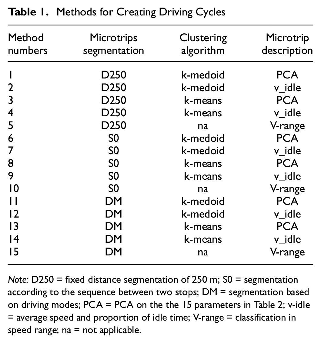
Note: D250 = fixed distance segmentation of 250 m; S0 = segmentation according to the sequence between two stops; DM = segmentation based on driving modes; PCA = PCA on the the 15 parameters in Table 2; v-idle = average speed and proportion of idle time; V-range = classification in speed range; na = not applicable.

Figure 1.

Variations in process for developing driving cycles.

Data Collection

Buses GPS data were provided by the Société de Transport de Montréal (STM), the Montreal Transit Authority. They cover five days of operation for five different buses, from Thursday November 8 to Monday November 12, 2018. From the data contained in the raw database, that is to say the second-by-second GPS position of the bus and instantaneous speed, the necessary information was deduced. The distance traveled and the average acceleration between each point as well as the date, time, and type of road (primary, secondary, tertiary, or residential) for each point were extracted. After the preprocessing, 24 h of tidy data were extracted for more than 450 km traveled.

Microtrip Generation

Three different methods of microtrip segmentation were selected based on what is most used in the literature or according to what is deemed to produce the most representative cycles. As shown in Figure 1, fixed distance segmentation of 250 m (D250), segmentation according to the sequence between two stops (S0), and segmentation based on driving modes (DM) were retained. A stop is defined as a sequence of null speed longer than 3 s. The DMs are itemized in Table 2 in the sub-section about time proportions of DMs. Figure 2 shows a speed profile divided by microtrips with each of the three selected methods. As we can see, S0 microtrip segmentation seems to produce longer microtrips than D250 and DM.

Table 2.

Characteristic Parameters (CP) of the Microtrips

	CP	Parameters	Unit
1	T	Segment duration	s
2	S	Travel distance	m
3	V	Average speed of the entire driving cycle	km/h
4	Vr	Average running speed	km/h
5	Vm	Maximum speed	km/h
6	Vstd	Standard deviation of speed	km/h
7	acc	Average acceleration of all acceleration phases	m/s²
8	dcc	Average deceleration of all deceleration phases	m/s²
9	A^2	Root mean square acceleration	m/s²
10	acc_std	Standard deviation of acceleration	m/s²
	Time proportions of driving modes:
11	Idle_p	Idle (speed = 0)	%
12	Acc_p	Acceleration (acceleration ≥0.1 m/s²)	%
13	Cru_p	Cruising (–0.1 m/s² < acceleration < 0.1 m/s², average speed > 20 km/h)	%
14	Dcc_p	Deceleration (acceleration ≤ –0.1 m/s²)	%
15	Cre_p	Creeping (–0.1 m/s² < acceleration < 0.1 m/s², average speed < 20 km/h)	%

Figure 2.

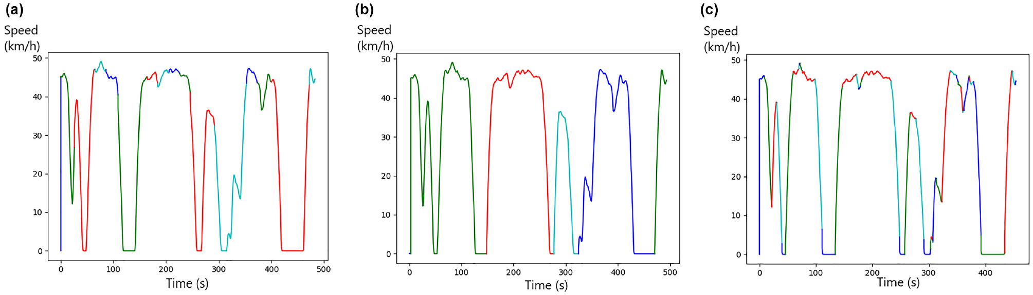
Speed profile with microtrip segmentation with: (a) D250, (b) S0, and (c) DM methods.

For each of the segmentation methods, a microtrip identifier is assigned to the data. Then, a second table is created with the microtrip identifier as an index and contains all the characteristic parameters of Table 2. The choice of microtrip characteristics is a combination of the selections made by ( 11 ) and ( 15 ).

Microtrip Classifications

As previously explained, clustering classifies microtrips into categories according to preselected characteristics. Two different clustering algorithms have been compared: k-medoid (PAM function of R) and k-means (k-means function of R). Both k-means and k-medoid algorithms imply the distribution of the data in several clusters, S₁, S₂, …, S_k, to minimize the sum of the squared distance between each point (x) and the center of its cluster (c). For the k-means algorithm the center of the cluster c is the barycentre, whereas for the k-medoid algorithm the center of the cluster c is the most central point inside the cluster.

In the literature, the number of clusters typically varies between 2 and 7. For example, ( 14 ) and ( 20 ) clustered their microtrips into seven clusters, ( 10 ) used three clusters, and ( 16 ) chose four clusters. In other studies, the silhouette value was used to determine the best number of clusters. The silhouette value allows the measurement of the quality of a clustering, calculating the average difference between the cohesion of a point and its separation from the nearest neighboring cluster. An average silhouette coefficient near 1 represents a high cohesion within the clusters. Yuhui et al. ( 15 ) performed the k-means clustering using two, three, and four clusters and selected two clusters because this configuration maximized the silhouette value. Preliminary results were done to select the number of clusters and to verify if the silhouette coefficient was a good indicator of driving cycle performance.

Moreover, the k-medoids and k-means algorithms require the definition of a distance measurement between the microtrips based on predefined characteristics. Two different ways of defining the microtrips and the distance between them have been compared. First, we describe the microtrips only according to their average speed and proportion of idle time—this is referred to as v_idle. The Euclidian distance between the standardized data couples is then used in the clustering algorithms. Figure 3a shows the clustered data for the seventh method with four clusters. Furthermore, microtrips were described using the 15 parameters in Table 2 and a PCA was applied. A PCA makes it possible to consider a large quantity of variables which are subsequently reduced to only a few main components by decorrelating them. The first four components were chosen as their accumulative contribution rate is 84.95% for the D250 segmentation, 92.55% for the S0 segmentation, and 84.66% for the DM segmentation, which is consistent with the generally accepted compression rates of 20% ( 11 )—this is referred to as PCA. Then, we clustered the microtrips using the Euclidian distance between the four principal components. Figure 3b shows a projection of the clustered data on the two main components for the first method with four clusters.

Figure 3.

(a) Clustering with the 7th method, (b) the 1st method, and (c) the 5th method.

As can be seen in the methodological scheme, we compared the performance of the two clustering methods with a classification in speed range (V-range). The microtrips were simply categorized according to their average speed in speed range which divides the interval [0,100] into 10 sub-intervals of equal length. Figure 3c shows the classified data in their speed range with the fifth method.

Selection of Assessment Measures

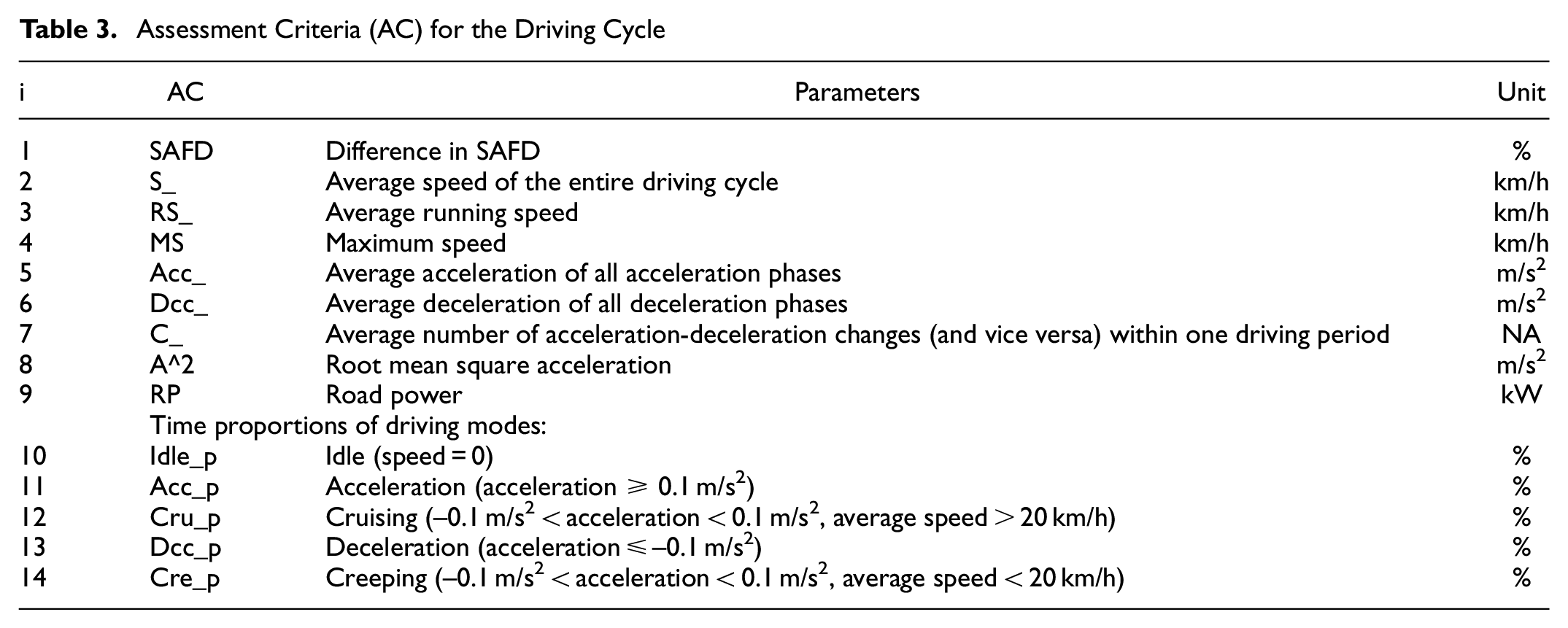
The assessment criteria chosen are those selected by ( 8 ), who followed the selection of criteria of ( 26 ). They are listed in Table 3. As previously explained, the SAFD is a matrix containing the speed acceleration time frequency distribution. The road power is computed in the same way as ( 26 ). The parameters have been computed for the entire database and are referred to as the targeted parameters TP_i. They also have been computed for every potential driving cycle and are referred as the cycle parameters CP_i.

Table 3.

Assessment Criteria (AC) for the Driving Cycle

i	AC	Parameters	Unit
1	SAFD	Difference in SAFD	%
2	S_	Average speed of the entire driving cycle	km/h
3	RS_	Average running speed	km/h
4	MS	Maximum speed	km/h
5	Acc_	Average acceleration of all acceleration phases	m/s²
6	Dcc_	Average deceleration of all deceleration phases	m/s²
7	C_	Average number of acceleration-deceleration changes (and vice versa) within one driving period	NA
8	A^2	Root mean square acceleration	m/s²
9	RP	Road power	kW
	Time proportions of driving modes:
10	Idle_p	Idle (speed = 0)	%
11	Acc_p	Acceleration (acceleration ≥ 0.1 m/s²)	%
12	Cru_p	Cruising (–0.1 m/s² < acceleration < 0.1 m/s², average speed > 20 km/h)	%
13	Dcc_p	Deceleration (acceleration ≤ –0.1 m/s²)	%
14	Cre_p	Creeping (–0.1 m/s² < acceleration < 0.1 m/s², average speed < 20 km/h)	%

Development of Driving Cycles

The Markov-chains approach is chosen for the development of the driving cycles as it is a widely used method ( 8 ). In our case, the entire database is used to develop a transition matrix between cluster types. A transition matrix is a square matrix containing the probabilities of transition from one event to another in a Markov process: it makes it possible to predict the future cluster knowing the present one. Therefore, after selecting a first microtrip randomly, the cluster of the following microtrip is determined using the transition matrix. The next microtrip is then randomly selected within the indicated cluster. These two steps are repeated until the cycle reaches its total length of at least 30 min. This time was chosen because it is in the interval of length of the existing driving cyles in past research.

Driving Cycle Selection

For each method presented in Table 1, the construction process is repeated several times. The number of iterations highly influences the representativeness of the produced driving cycle. Preliminary results have been executed in oder to choose the number of random walks. The relative difference (RD_i) between each of the assessment parameters of the obtained cycle (CP_i) and the targeted parameters (TP_i) is used to compare the cycles ( 21 ) and is calculated with Equation 1:

R D_{i} = | \frac{C P_{i} - T P_{i}}{T P_{i}} |

(1)

For all the assessment measures, the cycles specific to each method are sorted in ascending order according to their RDs. Then, as shown by Nouri and Morency ( 8 ), each cycle receives a rank according to its performance under each criterion. The cycle with the best total rank is designated as the candidate representative of its method. If the RD_i is below 5%, the level of similitude between the cycle and the database is considered to be high ( 7 , 14 ).

Results

Two preliminary tests have been conducted: first, the number of iterations needed to overcome the stochastic nature of the construction process has been estimated; second, the number of clusters for the k-means and k-medoids clustering algorithms has been identified. Then, with the selected number of iterations and number of clusters, the three segmentation methods, two clustering algorithms, and three microtrip descriptions have been compared looking at their ability to meet the assessment measures.

Selection of the Number of Iterations

As ( 21 ), we studied the evolution of the average RD for different numbers of iterations fixing the microtrip segmentation and clustering algorithm to the first method and fixing the number of clusters. We completed the entire process of building and selecting driving cycles several times for several iterations between 1 and 1,000. The objective was to identify the number of iterations where the performance of the selected cycle was steady. The performance was defined as the average RD and its variability was quantified by the standard deviation. Figure 4 shows the behavior of the average RD as a function of the number of iterations performed.

Figure 4.

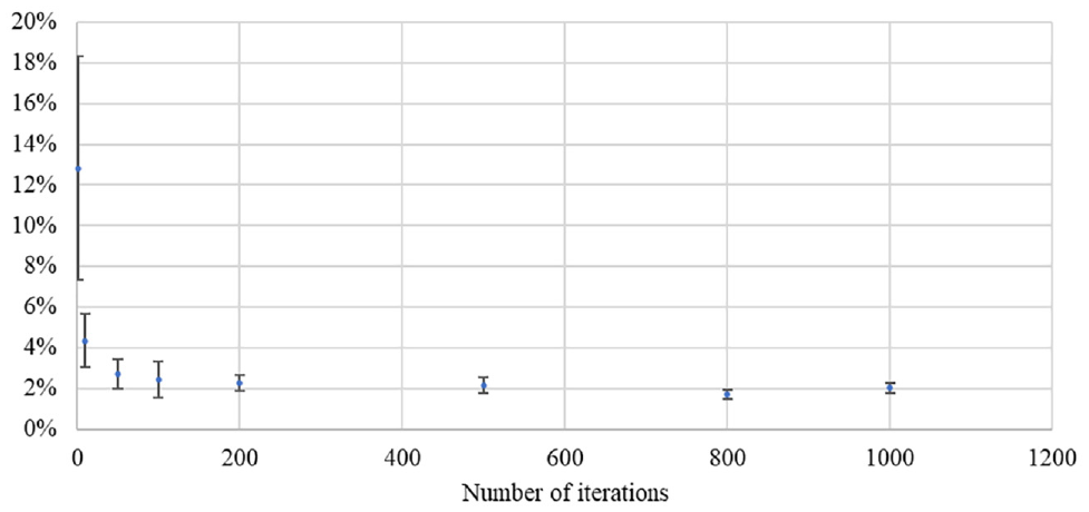
Average performance and standard deviation of the driving cycles for several numbers of iterations.

Because of the stochastic nature of the construction process, the performance of the driving cycle selected with several iterations between 1 and 10 was unpredictable and not reproducible. We noticed that the average performance of the obtained cycle varied very little between 50 and 1,000 iterations. On the other hand, the standard deviation was divided by 3 between 50 iterations and 800 iterations, going from 0.75% to 0.25%. There did not appear to be a gain in accuracy when the number of iterations increased to 1,000. The number of iterations was thus fixed at 800, because the precision associated with it will allowed a better comparison of the performance of the 15 methods with each other. Thus, we were able to set an uncertainty interval of 0.3% around our average RDs. Each criterion also had a specific margin of error listed in Table 4 based on its standard deviation evaluated with the first method.

Table 4.

Performance of the 15 Methods

Method:	1	2	3	4	5	6	7	8	9	10	11	12	13	14	15	Error
MS	39%	27%	43%	22%	30%	33%	35%	35%	36%	34%	0%	22%	0%	17%	17%	1%
S_	1.0%	4.5%	0.5%	0.4%	4.7%	4.4%	1.7%	3.6%	0.6%	1.2%	0.4%	10.8%	1.2%	5.6%	2.9%	0.9%
SAFD	1.3%	1.1%	1.3%	0.8%	1.3%	1.5%	1.6%	1.6%	1.7%	1.2%	0.9%	5.6%	0.3%	5.5%	6.4%	0.2%
Dcc_	2.7%	0.0%	3.5%	5.2%	0.6%	2.3%	1.3%	0.2%	2.0%	0.1%	0.2%	1.4%	1.7%	4.9%	5.2%	1.8%
Acc_	2.2%	1.6%	0.6%	4.1%	3.7%	2.4%	1.2%	2.3%	0.1%	4.0%	0.3%	5.9%	3.2%	9.4%	5.7%	1.2%
A^2	0.4%	1.0%	1.3%	1.5%	7.4%	0.4%	3.4%	0.7%	4.0%	2.3%	4.8%	0.1%	3.0%	5.0%	10.0%	1.0%
RP	5.0%	7.6%	2.3%	0.6%	5.5%	1.2%	0.3%	3.7%	0.6%	0.8%	0.3%	14.5%	1.9%	6.8%	4.4%	0.3%
RS	0.1%	2.7%	3.2%	0.2%	0.2%	1.9%	3.0%	3.5%	0.4%	0.3%	2.0%	9.0%	1.0%	6.1%	3.6%	0.4%
Idle_p	2.0%	3.4%	6.8%	1.1%	8.7%	4.6%	9.0%	0.3%	1.8%	2.8%	7.7%	6.6%	0.7%	1.7%	2.1%	1.5%
Acc_p	4.6%	1.3%	0.2%	1.2%	3.7%	1.8%	4.2%	1.6%	4.4%	4.5%	4.0%	0.3%	4.9%	3.2%	2.6%	1.2%
Dcc_p	1.0%	0.6%	0.3%	3.1%	1.1%	0.5%	1.7%	1.2%	0.7%	6.0%	4.2%	4.5%	1.4%	1.6%	2.9%	1.7%
Cru_p	1.8%	0.9%	0.1%	2.2%	1.3%	0.7%	3.1%	1.4%	2.7%	5.5%	0.0%	2.2%	1.6%	0.9%	2.5%	0.4%
Cre_p	1.8%	0.9%	0.1%	2.2%	1.3%	0.7%	3.1%	1.4%	2.7%	5.5%	0.0%	2.2%	1.6%	0.9%	2.5%	0.4%
C_	0.7%	6.5%	5.0%	10.2%	8.2%	11.2%	1.7%	2.8%	10.2%	1.5%	7.3%	0.3%	2.7%	1.9%	7.3%	2.2%
Mean RD	1.9%	2.5%	1.9%	2.5%	3.7%	2.6%	2.7%	1.9%	2.4%	2.7%	2.5%	4.9%	1.9%	4.1%	4.5%	0.3%
Rank	7	3	2	5	11	7	12	5	9	10	1	14	4	13	15
Rank\{MS}	4	3	1	8	11	6	12	5	9	10	2	14	6	13	15

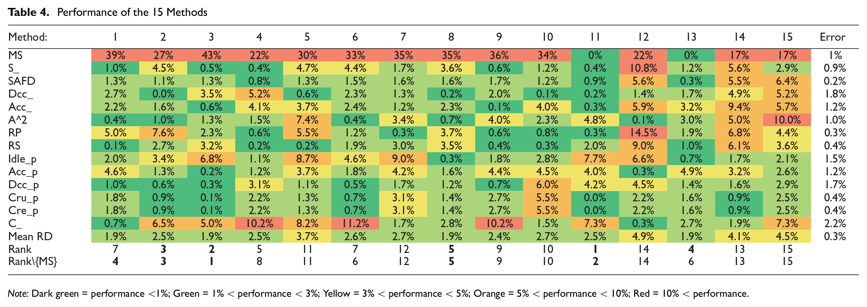
Note: Dark green = performance <1%; Green = 1% < performance < 3%; Yellow = 3% < performance < 5%; Orange = 5% < performance < 10%; Red = 10% < performance.

Selection of the Number of Clusters

A preliminary test made it possible to verify if the number of clusters used during k-means and k-medoids clustering was a good indicator of driving cycle performance. In other words, the test made it possible to verify if a silhouette coefficient close to 1, and therefore a more cohesive cluster configuration, corresponded to a better cycle according to the AC. Figure 5 shows the evolution of the silhouette value according to the number of clusters as well as the variation of the average RD for the first method. The three best RD performances occurred with eight, two, and three clusters for the first method and the best silhouette value performances occurred with two, three, and five clusters. Moreover, the silhouette value local maximas do not match with the average RD local minima. The same test was repeated for the sixth method and the clustering in eight categories stands out again only in the RD performance ranking. Therefore, the silhouette value does not appear to be a significant performance indicator to help in the selection of the number of clusters in the construction of the driving cycles. In addition, the standard deviation of the average RD is 0.55%, which means that the number of clusters has an impact on the performance of the driving cycle considering that for a particular method, the standard deviation is 0.3%. The number of clusters is fixed at eight for all the methods to be able to isolate the impact of microtrip definitions and clustering methods on the performance.

Figure 5.

Average relative difference (RD) and silhouette value according to the number of clusters for the first method.

Comparison of the 15 Combined Methods

As mentioned in the methodology, 15 different microtrip segmentation methods, clustering algorithm, and microtrip descriptions for distance measurement combinations were used to generate driving cycles. For each of the methods, 800 driving cycles were built and the best were selected according to their performance quantified by their RD. The RD_i of the best cycle of each method is presented in Table 4, as well as their average RD. The color spectrum makes it easy to visualize the best performences (green) and the worst performences (red). More precisely, values inferior to 1% are in dark green, those between 1% and 3% are in green, those between 3% and 5% are in yellow, those between 5% and 10% are in orange, and those higher than 10% are in red. The column error provides the margin of error specific to each criterion. To select the best method, the driving cycles representing each method are compared with the same ranking method explained in the section on the development of driving cycles. The average RD does not include the maximum speed RD_MS, which is always higher than 5%. This may be because data were not filtered a priori and that extreme values may not be valid. It is, therefore, not considered further.

To rank the methods, their respective cycles are compared with the same process used to select the best cycle within a construction method. The cycles are ranked in ascending numbers according to their RDs under each criterion. The ranks are summed within a method, and the final rank presented in Table 4 is determined by ranking these summed ranks.

As shown in Table 4, methods 2, 3, 11, and 13 stand out because of their good rank. By contrast, methods 7, 12, 14, and 15 have bad ranks and a high average RD. By grouping the methods with the same segmentation type and by calculating their total rank, we can observe that the D250 segmentation seems to be the best segmentation method, followed by the S0 segmentation and the DM segmentation methods. Because the SAFD is often considered to be particularly representative of the driving behaviors and relevant ( 21 ), this assessment measure deserves attention. The average SAFD was computed for each segmentation method and the results confirm the previous segmentation method ranking. The results are in agreement with those of the previous study conducted by Nouri and Morency ( 8 ). Moreover, the analysis shows that using a PCA on the 15 characteristic parameters of the microtrips presented in Table 2 yields the best performance, followed by the v_idle and V-range microtrip definition for distance measurement. The comparison of k-means and k-medoids clustering algorithm did not show any significant difference.

Conclusion

This study has proposed a systematic comparison of methods to develop driving cycles using a set of GPS data from a bus. As shown by this study, identifying the number of iterations required to have a valid cycle is a crucial step given the stochastic nature of the construction process. This study has demonstrated that 800 iterations seem to allow the performance of the selected cycle to be consistent. It was demonstrated for one method and presumed to hold for the others. Moreover, this study showed that the number of clusters in k-means and k-medoid algorithm has an impact on the performance of the final driving cycle, but that the silhouette value does not seem to be a good indicator of the final performance of the driving cycle. In this study, it was also confirmed that the segmentation with a fixed distance of 250 m is the best among the three tested segmentation methods. It was also discovered that the classification of the microtrips is better when they are characterized by many parameters as in Table 1, and then clustered via a clustering algorithm as k-means or k-medoid.

Further research will be required to confirm these results namely by increasing the size (days of observation), coverage (types of routes and roads sampled), and diversity (types of vehicles and data collection technology) of data used as input.

More consistent performances for a single method make it easier to compare them; therefore, additional methods could be evaluated. For example, the distance measure used by André ( 12 ), namely the chi-square distance on the SAFD, was not evaluated in this study, nor was the fuzzy C-means clustering method ( 10 ). The impact of cycle length and cycle covered distance could also be studied. Moreover, as emphasized by Xiao et al. ( 7 ) and done by ( 17 ), it would be relevant to study the performance of cycles by evaluating their ability to predict emissions using fuel rate data, for example by including the fuel consumption as an assessment criteria.

Footnotes

Acknowledgements

The authors acknowledge the support of the Société de Transport de Montréal in providing access to data for research purposes as well as of the Mobilité Chair Partners for their support.

Author Contributions

The authors confirm contribution to the paper as follows: study conception and design: Roy and Morency; data collection: Société de Transport de Montréal; analysis and interpretation of results: Roy and Morency; draft manuscript preparation: Roy and Morency. All authors reviewed the results and approved the final version of the manuscript.

Declaration of Conflicting Interests

The author(s) declared no potential conflicts of interest with respect to the research, authorship, and/or publication of this article.

Funding

The author(s) disclosed receipt of the following financial support for the research, authorship, and/or publication of this article: This research was funded by NSERC.

References

United States Environmental Protection Agency. Global Greenhouse Gas Emissions Data. EPA. https://www.epa.gov/ghgemissions/global-greenhouse-gas-emissions-data. Accessed April 13, 2017.

Ministère de l’environnement et de la lutte contre les changements climatiques. Inventaire québécois des émissions de gaz à effet de serre en 2016 et leur volution depuis 1990. Québec, 2018.

Société de transport de Montréal. Rapport d’activité 2018. Montreal, 2019.

Aéroports de Montréal. Rapport annuel 2017. Montréal, 2018.

Mundy

Trompet

Cohen

Graham

The Identification and Management of Bus Priority Schemes: A Study of International Experiences and Best Practices. Imperial College London, Railway and Transport Strategy Centre, 2017.

Karekla

Fernandez

Tyler

Environmental Effect of Bus Priority Measures Applied on a Road Network in Santiago, Chile. Transportation Research Record: Journal of the Transportation Research Board, 2018. 2672: 135–142.

Xiao

Dui-Jia

Jun-Min

A Synthesis of Methodologies and Practices for Developing Driving Cycles. Energy Procedia, Vol. 16, 2012, pp. 1868–1873.

Nouri

Morency

Evaluating Microtrip Definitions for Developing Driving Cycles. Transportation Research Record: Journal of the Transportation Research Board, 2017. 2627: 86–92.

Koossalapeerom

Satiennam

Leelapatra

Seedam

Rakpukdee

Comparative Study of Real-World Driving Cycles, Energy Consumption, and CO2 Emissions of Electric and Gasoline Motorcycles Driving in a Congested Urban Corridor. Sustainable Cities and Society, Vol. 45, 2019, pp. 619–627.

10.

Zhao

Wang

Developing an Electric Vehicle Urban Driving Cycle to Study Differences in Energy Consumption. Environmental Science and Pollution Research, Vol. 26, No. 14, 2018, pp. 13839–13853.

11.

Peng

Zhuang

Yang

A Driving Cycle Construction Methodology Combining K-Means Clustering and Markov Model for Urban Mixed Roads. Proceedings of the Institution of Mechanical Engineers, Part D: Journal of Automobile Engineering, Vol. 234, No. 2–3, 2019, pp. 714–724.

12.

André

The ARTEMIS European Driving Cycles for Measuring Car Pollutant Emissions. Science of the Total Environment, Vol. 334–335, 2004, pp. 73–84.

13.

Wang

Zhang

Liu

Driving Cycle Construction for Electric Vehicles Based on Markov Chain and Monte Carlo Method: A Case Study in Beijing. Energy Procedia, Vol. 158, 2019, pp. 2494–2499.

14.

Zheng

Zhou

Real-World Driving Cycles and Energy Consumption Informed by Large-Sized Vehicle Trajectory Data. Journal of Cleaner Production, Vol. 223, 2019, pp. 564–574.

15.

Yuhui

Yuan

Huibao

Development of a Representative Driving Cycle for Urban Buses Based on the K-Means Cluster Method. Cluster Computing, Vol. 22, No. 3, 2017, pp. 1–10.

16.

Fotouhi

Montazeri-Gh

M. J.

Tehran Driving Cycle Development using the K-Means Clustering Method. Scientia Iranica, Vol. 20, No. 2, 2013, pp. 286–293.

17.

Quirama

L. F.

Giraldo

Huertas

J. I.

Jaller

Driving Cycles that Reproduce Driving Patterns, Energy Consumptions and Tailpipe Emissions. Transportation Research Part D: Transport and Environment, Vol. 82, 2020, p. 102294.

18.

Huertas

J. I.

Quirama

L. F.

Giraldo

M. D.

Díaz

Comparison of Driving Cycles Obtained by the Micro-Trips, Markov-Chains and MWD-CP Methods. International Journal of Sustainable Energy Planning and Management, Vol. 22, 2019, pp. 109–120.

19.

Lin

Niemeier

D. A.

An Exploratory Analysis Comparing a Stochastic Driving Cycle to California’s Regulatory Cycle. Atmospheric Environment, Vol. 36, No. 38, 2002, pp. 5759–5770.

20.

Nouri

Enhancing the Gasoline Vehicles’ CO2 Emissions Estimation in Montreal. Doctoral dissertation. École Polytechnique de Montréal, 2015.

21.

Huertas

J. I.

Quirama

L. F.

Giraldo

Díaz

Comparison of Three Methods for Constructing Real Driving Cycles. Energies, Vol. 12, No. 4, 2019, p. 665.

22.

Nyberg

Frisk

Nielsen

Using Real-World Driving Databases to Generate Driving Cycles with Equivalence Properties. IEEE Transactions on Vehicular Technology, Vol. 65, No. 6, 2016, pp. 4095–4105.

23.

Gong

Zou

Yang

Fan

Sun

Goehlich

Generation of a Driving Cycle for Battery Electric Vehicles: A Case Study of Beijing. Energy, Vol. 150, 2018, pp. 901–912.

24.

Kamble

S. H.

Mathew

T. V.

Sharma

G. K.

Development of Real-World Driving Cycle: Case Study of Pune, India. Transportation Research Part D: Transport and Environment, Vol. 14, No. 2, 2009, pp. 132–140.

25.

Wang

Qiao

Approach to Development and Evaluation of Driving Cycles for Classified Roads Based on Vehicle Emission Characteristics. Transportation Research Record: Journal of the Transportation Research Board, 2008, 2058: 58–67.

26.

Ashtari

Bibeau

Shahidinejad

Using Large Driving Record Samples and a Stochastic Approach for Real-World Driving Cycle Construction: Winnipeg Driving Cycle. Transportation Science, Vol. 48, No. 2, 2014, pp. 170–183.