
Abstract
High-resolution vehicle trajectory data can be used to generate a wide range of performance measures and facilitate many smart mobility applications for traffic operations and management. In this paper, a Longitudinal Scanline LiDAR-Camera model is explored for trajectory extraction at urban arterial intersections. The proposed model can efficiently detect vehicle trajectories under the complex, noisy conditions (e.g., hanging cables, lane markings, crossing traffic) typical of an arterial intersection environment. Traces within video footage are then converted into trajectories in world coordinates by matching a video image with a 3D LiDAR (Light Detection and Ranging) model through key infrastructure points. Using 3D LiDAR data will significantly improve the camera calibration process for real-world trajectory extraction. The pan-tilt-zoom effects of the traffic camera can be handled automatically by a proposed motion estimation algorithm. The results demonstrate the potential of integrating longitudinal-scanline-based vehicle trajectory detection and the 3D LiDAR point cloud to provide lane-by-lane high-resolution trajectory data. The resulting system has the potential to become a low-cost but reliable measure for future smart mobility systems.
Traffic operations and management rely heavily on the traffic data collected from intersections and roads. Efficient and reliable traffic sensing and detection empower traffic managers to measure and assess traffic conditions objectively, mitigate traffic congestion, and adjust traffic signal timing. With high-resolution vehicle trajectory data, we can effortlessly estimate intersection delay, travel time, Level of Service (LOS), and so forth. The trajectory data can contribute to incident management, active traffic control, and speed harmonizing, improving the safety and mobility—ranging from individual intersections to the entire roadway network. In the era of connected and autonomous vehicles (CAV), vehicle trajectories obtained from roadside sensors play a critical role for many V2I (Vehicle to Infrastructure) applications such as Cooperative Adaptive Cruise Control, Dynamic Merge Assistance, and Eco-Traffic Signal Timing. However, many current traffic sensing technologies cannot satisfy the data needs of CAV applications. For instance, GPS position data can have errors up to a few meters, which is not sufficiently accurate for vehicle positioning. In this paper, we developed a LiDAR-Camera system to extract vehicle trajectories from traffic video and then generated physical vehicle positions by mapping the 2D video to 3D LiDAR data, considering recent trends of integrating 3D infrastructure data into infrastructure management and maintenance.
Recently, transportation infrastructure data has evolved from 2D map data into the high- definition (HD) 3D map data. These HD map data contain rich spatial information and can provide detailed infrastructure information for multi-resolution and multi-level analysis. Leading technology companies, as well as public agencies, are now shifting to 3D point cloud data for modeling complex urban environments. For instance, 23 state Departments of Transportation in the United States reported having already transitioned to 3D modeling for Civil Integrated Management (CIM) including Utah, Washington, and Oregon ( 1 ). With the growing number of 3D map applications, users such as infrastructure administrators, government agencies, and researchers can now access a large amount of point cloud data.
This paper makes two major contributions. On the one hand, a new longitudinal scanline-based trajectory detection model is developed for the more complex arterial intersection environment to provide high-resolution vehicle trajectory data in traffic videos. The new model uses an integrated adaptive background and foreground subtraction method to cope with the complex noise conditions found at arterial intersections. On the other hand, the 3D infrastructure point clouds collected by static LiDAR scanning were used to convert pixel trajectories in video footage to real-world trajectories by matching feature points between the 2D video image and the 3D infrastructure point cloud. The combination of 3D infrastructure data and computer vision can provide a low-cost, high-accuracy, and more scalable solution for data collection in traffic operations and smart mobility applications.
Literature Review
Traffic Video Analytics
Compared with many other traffic sensing devices, traffic cameras have apparent advantages, which can make them a cost-effective solution in the service of the infrastructure-based detector. Because of their capability to provide rich information and a large coverage area, CCTV Cameras have been applied for vehicle speed measurement, traffic analytics, near-miss reporting, and incident review. Their main disadvantage is that vision sensors are sensitive to illumination changes. The video image processing relies on external illumination, resulting in lower accuracy at night. To resolve this issue, the video image detector is often used together with other types of detectors to provide some level of backup, such as Radar or Remote Traffic Microwave Sensor (RTMS).
Existing video-based vehicle detection and recognition methods can be categorized as either motion-based methods or model-based methods. The motion-based method employs motion information to segment moving objects from the traffic scene between consecutive frames. In contrast, the model-based approach identifies objects based on their appearance using a pre-trained template. Typical motion-based methods include frame differencing, background subtraction, and the optical flow method. Model-based methods include a Histogram of Gradient (HOG) feature detector ( 2 ), Deformable Part Model ( 3 ), and deep learning models ( 4 , 5 ). The rise of AI and deep learning has significantly advanced image object detection in recent years. However, deep learning models usually demand a substantial amount of training data, severe computational cost, and sophisticated model design.
Another commonly seen traffic video analysis is scanline based. A scanline is a group of pixels on selected lanes, which are used for object detection and tracking. There are two types of scanline. One is the latitudinal scanline, which is defined across the traveling path ( 6 – 9 ). The other is the longitudinal scanline that is defined along the traveling direction ( 10 – 12 ). Most of the previous scanline-based vehicle detection can only produce spot-specific traffic parameters, such as volume, vehicle type, and spot speed.
A recent study by Zhang and Jin ( 13 ) explored the potential of using a High Angle Spatial-Temporal Diagram Analysis (HASDA) model to generate high-resolution vehicle trajectories with longitudinal scanlines defined on the centerlines of traffic lanes. The proposed model was developed for traffic video scenarios like those from the NGSIM (Next-Generation Simulation) project. However, directly applying HASDA to medium-angle intersection traffic video can be quite challenging. HASDA raises several key issues. First, the pixel-to-physical coordinate transformation methods that require manually picking and measuring the distance along the direction of traffic in HASDA will be inefficient for arterial intersection scenarios with curved vehicle trajectories for turning movements and pan-tilt-zoom (PTZ) operations by roadside cameras. Second, the noise conditions at arterial intersections are much more complex, especially considering that an intersection is a space shared by vehicles and pedestrians and the amount of traffic control devices, markings, and wirings at the intersection. Third, with medium-angle cameras, the vehicle occlusions become more severe. Finally, vehicle trajectories at arterial intersections have more frequent stop-and-go trajectories because of signal control. In this paper, a LiDAR-Camera (3D-2D) matching method is proposed to address the coordinate transformation issues. An improved video processing model is proposed with significant enhancement on most of the modules in the HASDA model to address the image processing challenges for medium-angle arterial intersection traffic video.
Traffic Camera Calibration
Camera calibration is to provide a mapping relationship between real-world coordinates and a 2D image, which is the foundation for extracting vehicle trajectories, measuring speeds, and acquiring other traffic information from video footage. Some camera calibration techniques require detection of the vanishing point (VP) in the 2D image, which is the point on the image plane formed by the convergence of mutually parallel lines in three-dimensions. Others are using reference objects to calculate the camera pose based perspective transformation. Dailey, Cathey, and Pumrin ( 14 ) developed an algorithm to estimate mean traffic speed from uncalibrated cameras without knowing information such as camera focus, tilt, or angle. Their algorithm is constrained to several assumptions, such as the limitation of the speed of the vehicle, motion constraints on the road plain, linear change of the scale factor, and known vehicle length distribution. Schoepflin and Dailey ( 15 ) presented a three-stage method to calibrate the roadside camera to turn it into a speed sensor for traffic management. Their model used the motion of the vehicle to estimate the camera position and calibrated the camera by determining the VP of the roadway. Cathey and Dailey ( 16 ) proposed an algorithm to calibrate a PTZ camera, consisting of three phases: (1) lane boundary detection, (2) computation of VP and image straightening transformation, and (3) calculation of the image-to-highway scale factor (feet per pixel). Grammatikopoulos, Karras, and Petsa ( 17 ) developed an approach for the automatic estimation of camera parameters (camera constant, location of principal point, and two coefficients of radial lens distortion) from images with three VPs of orthogonal directions. Dubská et al. ( 18 ) proposed a fully automatic camera calibration method without the manual setting under various road conditions. Their approach detects and tracks local feature points of moving vehicles and uses the trajectories of tracked points to obtain VP corresponding to the direction of moving vehicles. Luvizon et al. ( 19 ) used the planar of the inductive loop detector as a reference object to construct a homography matrix for measuring vehicle speed from license plate detection. Do et al. ( 20 ) developed a method of calibration to measure traffic speed by drawing an equilateral triangle on the ground as a 2D reference object. Then they solve the three configuration parameters of height h, the tilt angle ψ, and the focus distance f. You and Zheng ( 21 ) developed a dynamic calibration method by obtaining two VPs, namely the VP in the direction of the lane traveled and the orthogonal vanishing point. More recently, Sochor et al. ( 22 ) developed a deep learning model to assign a 3D bounding box for the detected vehicle. Based on the outputs of the deep learning model, they can obtain two vanishing points for camera calibration. Their result reduced the distance ratio error of vanishing point detection from 0.18 to 0.09, which beat the previous state-of-the-art model. Sochor et al. ( 23 ) established a benchmark dataset for evaluating different traffic camera calibration methods. The speed of vehicles in the dataset was collected using LiDAR and verified through GPS trackers. Bhardwaj et al. ( 24 ) proposed the AutoCalib system for scalable, automatic calibration of traffic cameras, using a deep learning model to extract selected key-point features from vehicle images to produce a robust estimate of the camera calibration parameters automatically. Their model relies on the car’s known geometric parameters (e.g., the distance between the two taillights).
Some of the traffic camera calibration methods mentioned above are based on VPs inferred from moving objects, which make those models sensitive to environmental variations. Other models that are based on reference objects are hard to deploy in practice because traffic operators cannot move the reference object every time the PTZ camera scene changes.
Mobile LiDAR Technology and LiDAR-Camera Integration
LiDAR sensors, including mobile LiDAR, airborne, and static LiDAR, have been used extensively in transportation studies like vehicle and pedestrian detection, object localization, and trajectory tracking. LiDAR-based mapping services and sensing technology play a critical role in self-driving vehicles executing complex maneuvers. A wide range of spatial information can be extracted from LiDAR point cloud data including road level (e.g., road surface, lane markers, driving lines, cracks, and manholes), object-level analysis (e.g., buildings, trees, vehicles, and power lines), to building-structure element level analysis (e.g., façade, doors, windows, roofs).
A lot of research has explored the use of LiDAR for automated urban on-road object detection and extraction ( 25 – 27 ). For example, Zai et al. ( 28 ) proposed an effective 3D road boundary extraction by employing super-voxels and graph cuts on MLS (Mobile LiDAR System) data. Other studies, such as Xu et al. ( 29 ), developed a method for automatic extraction of road curbs and evaluated their method on a large scale of residential and urban area mobile LiDAR point clouds. Additionally, Yang et al. ( 30 ) presented a technique that can realize the automated extraction of road markings from mobile LiDAR point clouds. In this study, 3D point clouds were converted into 2D geo-referenced feature images, and road markings were filtered by controlling LiDAR intensity and elevation value. Finally, road marking outlines were extracted, based on prior knowledge of road marking shape and arrangement. Yu et al. ( 31 ) proposed an algorithm using a multi-thread computing strategy to detect urban road manhole covers with MLS data. Other published studies focus on automated urban object extraction, including traffic signs, trees, buildings, vehicles, powerlines, and so forth ( 32 – 35 ). Yang et al. ( 36 ) proposed a method for urban object extraction with mobile LiDAR data. They generated multi-scale super-voxels and reduced computing costs by segmenting super-voxels. Finally, their approach was validated with large datasets and achieved accuracy between 90% and 96%. Some studies focus on the building element extraction from MLS data. For example, MLS data have been successfully used in window and façade detection in the study of Wang et al. ( 37 ) and Arachchige et al. ( 38 ).
Another important topic about LiDAR is the sensor fusion of LiDAR and camera, which has received increasing attention over the years. Cameras can provide rich texture and color information, while LiDAR can provide accurate spatial data. When fusing them, it can provide depth information for the pixels in the camera image with reliable 3D point clouds, which are useful in velocity estimation for precise vehicle tracking and autonomous driving. Extensive studies have been explored on the registration between LiDAR and camera imagery. The most common approaches require the existence of known targets in the scene ( 39 – 43 ). In these studies, checkerboards and other types of target (e.g., triangles, circles, or white-to-black transitions) that are observable by both LiDAR and camera were used. For example, Zhang et al. ( 39 ) exploited a planar checkerboard and used nonlinear least-squares optimizations to calibrate a single optical camera with a 2D scanner. In a study by Narodistsky et al. ( 42 ), the calibration problem is described as a set of polynomial equations, and six correspondences are minimally required for the alignment of the LiDAR-Camera system. Recently, more research has attempted to automate the calibration process using features in the observed scene, without markers or targets. For example, Pandey et al. ( 44 ) addressed automatic targetless extrinsic calibration by maximizing mutual information between the image and the 3D LiDAR-Camera. It used the known intrinsic value of the camera and estimated the extrinsic parameters to project LiDAR onto camera imagery. The mutual information value was computed by comparing the LiDAR reflectivity with the intensities value from camera images. In another study proposed by Li et al. ( 45 ), the registration of a panoramic image sequence and mobile laser scanning point clouds in the urban environment were estimated by using parked vehicles as registration primitives.
In contrast, there has been minimal research on PTZ camera calibration using infrastructure 3D LiDAR data for vehicle trajectory detection. Previously published studies of the combination of LiDAR (for range information) and camera systems (“for better recognition”) have focused on the dynamic data fusion between image objects detected in traffic video and the corresponding 3D point cloud clusters identified in mobile LiDAR data.
In this paper, the focus is to use the static LiDAR 3D point cloud to assist the physical trajectory extraction. The camera and LiDAR capture data at the same time and in the same location in existing papers ( 43 – 45 ). Those methods assume the LiDAR-Camera alignment can be accurately estimated when the camera and LiDAR are capturing the same scene on a mobile platform. Such an assumption cannot apply to the proposed LiDAR-Camera system for vehicle trajectory detection. In this paper, the traffic cameras capture the dynamic roadway conditions, while the pre-collected static LiDAR 3D model is used as the basis for mapping pixel trajectories to 3D coordinates.
Methodology
Overall Workflow
The proposed model will use both static and dynamic data for vehicle trajectory generation. The overall workflow is illustrated in Figure 1. As a preprocessing step, the 3D infrastructure point cloud data are used to establish coordinate transformation matrices between video and physical coordinates. The main video analytic workflow is depicted on the left branch in which raw video data are processed and analyzed to generate pixel trajectory, while the right branch uses LiDAR data to conduct 2D-3D matching to convert the pixel coordinates into State Plane Coordinates for the generation of physical trajectories.

Dataflow of LiDAR-assisted longitudinal-scanline-based traffic video analysis.
Scanline-Based Trajectory Extraction
The scanline-based trajectory extraction consists of four main steps, including the spatial-temporal map (ST Map) generation, preprocessing, vehicle strand detection, and pixel trajectory detection.
Scanline Generation
Scanlines are defined as the centerline of traveling lanes within the detection areas. They consist of a complete pixel line
Bresenham’s Line Pixel Algorithm
Input: Given two consecutive control points
Outputs: The set
Algorithm:
Initialization:
Calculate the STLine pixel spans and directions for x and y coordinates, respectively:
where
Point Generation:
Initialize the STLine point set
If
For
If
Else:
Add
Else (
For
If
Else:
Add
Add Endpoint
Figure 2 illustrates the user-defined scanlines in the tested videos, which covered nine lanes at the signalized intersection next to a train station to be used for model evaluation.
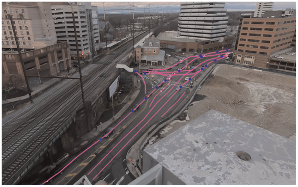
Scanlines defined at the experimental intersection site near a train station.
Spatial-Temporal Map Generation
An ST Map
where
The ST Map preserves trajectories of any moving objects passing along the scanline over time. Each moving object will leave a trace that shows the path of the object, which is named as vehicle strands. Each strand on the ST Map represents a unique vehicle, as illustrated in Figure 3. By using ST Maps for vehicle trajectory extraction, the conventional two-step trajectory extraction algorithm consisting of object detection and tracking over the full video footage is simplified as a one-step algorithm of segmenting out the vehicle strands on ST Maps.
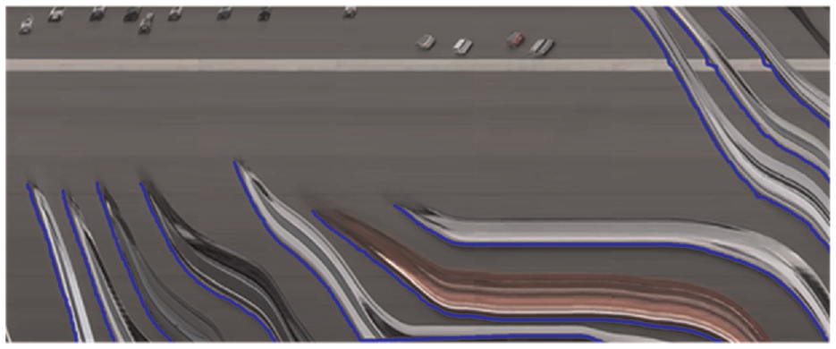
ST Map and vehicle trajectories.
ST Map Preprocessing and Shadow Removal
Preprocessing modules are necessary to remove the noise before trajectory extraction, such as shadow removal and background subtraction. However, because of the complexity of the scene at the arterial intersections, a more adaptive background subtraction method is proposed to segment out vehicle strands.
The shadow removal module uses a 3-by-3-pixel neighborhood area to search for low-intensity and texture-free areas that are induced by shadows. The shadow removal results can be found in Figure 4.

Sample results of shadow detection on ST Map.
ST Map Background Subtraction and Vehicle Strand Detection
One key challenge of computer vision on arterial intersection video is its complex environment where hanging wires, lane markings, roadside objects, and crossing vehicles can all leave irregular stains that can affect trajectory detection. However, ST Map has a useful characteristic in that its background stays relatively stable, and the normal changes in the background are gradual. Applying background detection to ST Maps becomes feasible and more efficient than conventional frame-by-frame background subtraction methods. This is a major improvement from the HASDA ( 13 ) model in which the targeted freeway scenes have mostly uniform pavement colors.
In the proposed model, three major features, including edge features, color features, and motion features are fully integrated as an adaptive model for the complex conditions of varying road surface color, infrastructure noise conditions, and the traces of crossing traffic. The three modules work as follows.
Adaptive Background Detection and Noise Removal
We assume that the intensity level of the roadway pavement and other static objects (e.g., light poles, cables, lane markings) follows a normal distribution, while the vehicle textures are usually randomly distributed, which is shown in a histogram in Figure 5a. Different from HASDA ( 13 ), only one background color range is used for the entire video because of the uniform color of each freeway lane. The background scene studied in the proposed model often has multiple colors, even on the same STLine. Therefore, an adaptive background color thresholding method is proposed to process the background subtraction on each line of the ST Map.

Histogram thresholding based background detection method and sample results: (a) a normal distribution with the vehicle textures randomly distributed, (b) a typical ST Map background from an arterial scanline with multi-layer colors and different types of static noises; (c) the results of replacing all background pixels with the uniform color.
The probability of any intensity level

where
The intensity of roadway pavement and intensity of vehicle strands often occupy different ranges on the histogram. Considering that the background roadway is the majority, the road pixel intensities can be defined by background thresholds
Algorithm: Histogram Based Background Detection
RGB Spatial-Temporal Map:
Spatial-Temporal Map with uniform Background:
Compute the median RGB value of ST Map
Convert S to Gray level image G.
Compute the histogram of intensity distribution H(r)
Find the valleys of H(r) on both sides as (
Set
Figure 5b shows a typical ST Map background from an arterial scanline with multi-layer colors and different types of static noises. Figure 5c shows the results of replacing all background pixels with the uniform color.
The background detection module is the most critical part of the scanline algorithm. In the previous HASDA method ( 13 ), the background thresholding method was applied against the entire ST Map. However, the assumption of the previous method does not hold in the new scenario as the pavement color along the scanline may not be consistent because of the complex surrounding environment. In this paper, the histogram thresholding method was applied for each row on the ST Map, considering that the color of each row does not vary within a certain time interval. Although the ST Map from a complex intersection can be untidy because of additional noise. We can easily clean out the static noise and ghost vehicle strands by applying the histogram thresholding method as shown in Figure 6.

Before-after histogram thresholding: (a) original ST Map with multi-layer background noises and static noises, and (b) cleaned ST Map after adaptive row-by-row background thresholding.
Edge Detection based Strand Detection
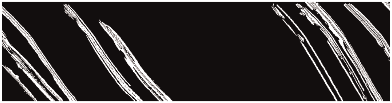
The edge detection methods are similar to those used in HASDA ( 13 ). The Canny edge detector is used to detect edges across different directions adaptively. However, the outputs of the Canny edge detector are incomplete and often lead to cracked segments, as is shown in Figure 7. Some additional morphological operators are applied to fill the small gaps in-between detected edges to form the vehicle strands.
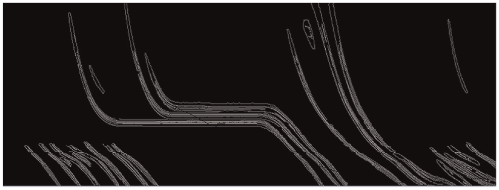
Sample edge detection results for vehicle strands.
ST Map Time Differencing
Time differencing on the ST Map is defined as the maximal absolute differences of RGB colors between two neighboring columns on the ST Map
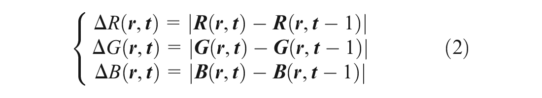
where

Figure 8 shows a sample time differencing result.
Sample strands detection results using time differencing.
After background detection, edge detection, and time differencing, we combine the three results together to obtain the foreground vehicle strands. Then a connected component labeling is used to connect all 8-direction connected foreground areas.
Connected-Component-Based Denoising
In the HASDA ( 13 ) model, because of the cleanness of the freeway scene, the connected components only need minor image morphological operations. In arterial intersection scenarios, the connected components generated from vehicle strand detection still contain noise from crossing traffic and residuals of background subtraction.
Background residuals: In the proposed algorithms, a moving window is defined to detect and remove horizontal background noise. If there is a horizontal line with a length longer than 1/2 of the window, then the static line is identified. The detected line is then compared with a vertical threshold, for example, 10 pixels, to ensure it is not induced by stopped vehicles at intersection or congestion.
Figure 9a shows a residual background noise from a static object. The noise was removed through the moving-window-based line detection and removal.
Crossing traffic: Crossing vehicles are typically small foreground areas with limited temporal span. Thresholds on the total pixel count and the duration of a connected area are used to eliminate those crossing traffic noises. Figure 10 illustrates how those crossing vehicles are identified and removed with the crossing traffic removal module.
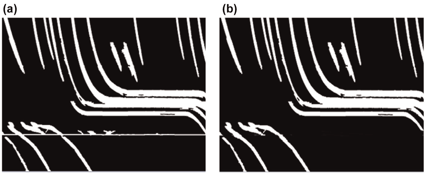
Sample results for background residual noise removal: (a) binary connected components with horizontal noises, and (b) clean binary connected components of vehicle strands.
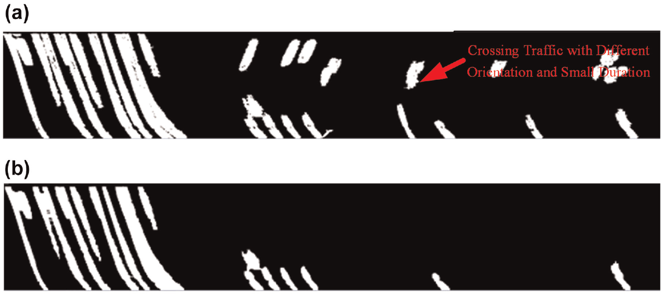
Sample results for crossing traffic removal: (a) binary connected components with crossing traffic; and (b) binary connected components after removing crossing traffic.
Pixel Trajectory Extraction
Similar to the pixel trajectory extraction methods in the HASDA model, we extract trajectory by detecting the bottom-left edges of vehicle strands. The edges of vehicle strands correspond to the movement of the front bumpers of vehicles. Therefore, the complete movement of the car along the scanline can be obtained. On completion of trajectory profiles on the ST Map, we can acquire the vehicle trajectories in video image coordinates, as we know the video pixel coordinates of all points of the scanline. The results of generated trajectory profiles on the ST Map are plotted in Figure 11.
Sample detected pixel trajectories on ST Map.
Several post-processing modules were added to the HASDA vehicle trajectory extraction algorithm to fix some irregularities in the detected vehicle trajectories.
Backward travel removal: The connected trajectories are processed to ensure no background traveling occurs by always setting the final pixel trajectory

where
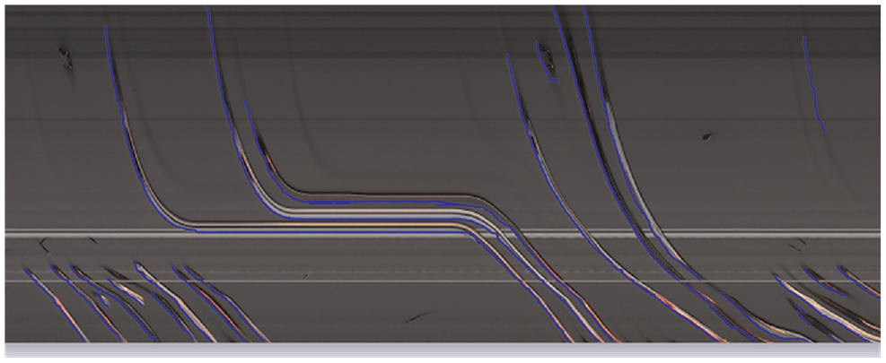
Zigzagging removal: Zigzagging is a phenomenon when two close-by vehicle trajectories have broken pieces that may be interconnected.
As illustrated in Figure 12a, two trajectories, one from a stopped vehicle at the intersection and another from an approaching vehicle upstream, are stitched together, resulting in zigzagging. Some motion constraints used to prevent the zigzag connections between two trajectories. After processing the zigzagging trajectory, the trajectory vehicle is realistic, as shown in Figure 12b.
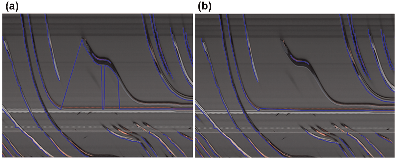
Sample cleaning results for zigzagging trajectories: (a) trajectories with zigzagging, and (b) cleaned trajectories.
LiDAR Processing and Camera Calibration
Estimating Video Distortion
Correcting the lens distortions is critical to an accurate projection result. Without a reasonable estimate of the camera distortion, it is difficult to calculate the precise projection between the video frame and point cloud. The camera calibration and lens un-distortion steps are implemented with the OpenCV toolbox.
Raw LiDAR Processing
The New Brunswick mobile LiDAR dataset is hosted in the online mapping system (Figure 13b). LiDAR data can be retrieved by entering the GPS information of the study area (40.496326 N and –74.446131 W). The raw LiDAR point cloud obtained from the online mapping system is shown in Figure 13d. After this step, we first removed the highlighted building in Figure 13c, which blocks the studied area (see Figure 13e). Then, we removed the point cloud out of the camera view and cleaned the target area by eliminating the noise points, and the points belong to vehicles, pedestrians, trees, and so forth. The point cloud model study area after cleaning is shown in Figure 13f.
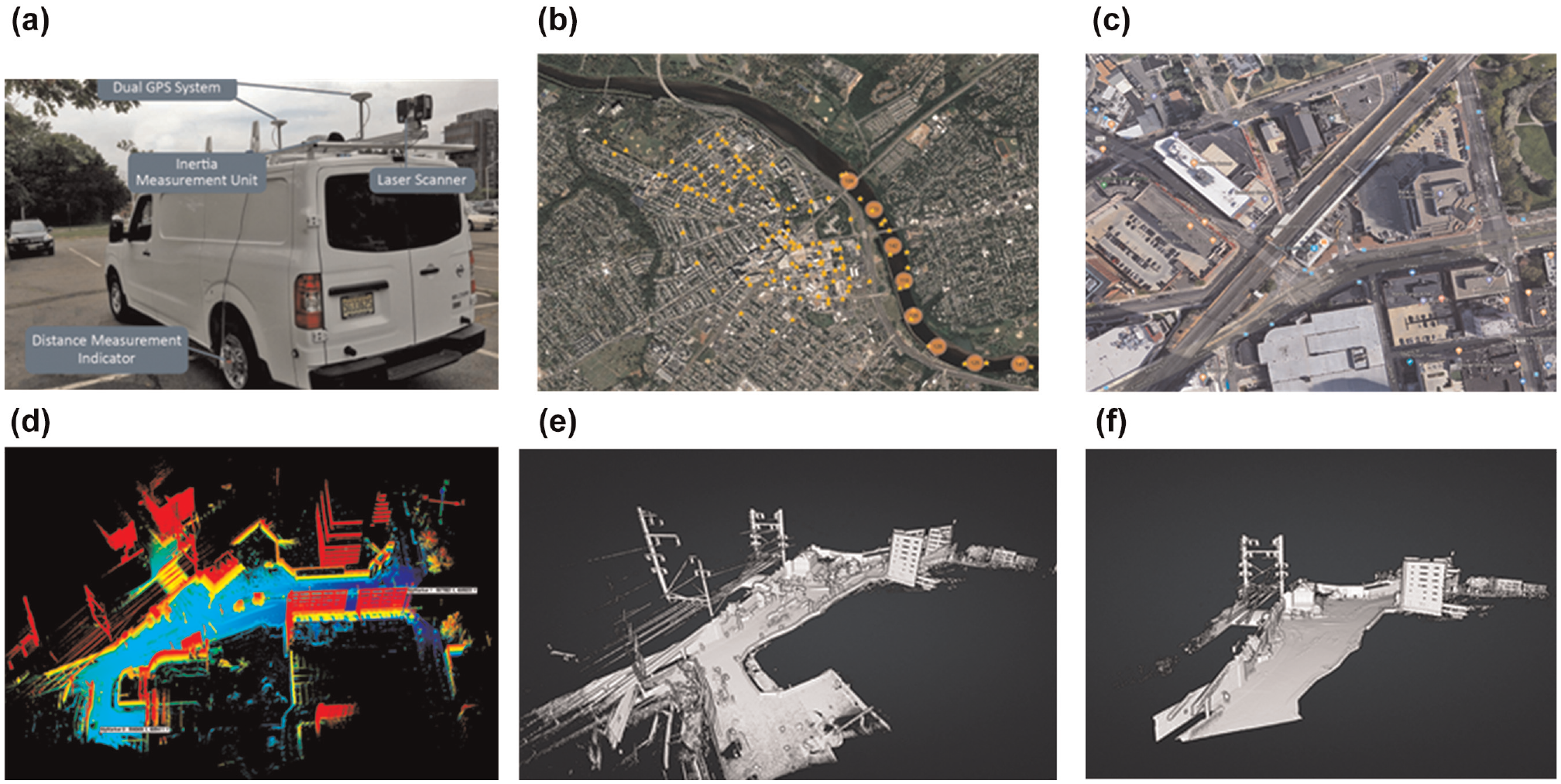
Demonstration of the mobile LiDAR based 3D infrastructure point cloud data collection and processing: (a) Rutgers mobile LiDAR system, (b) New Brunswick mobile mapping database, (c) study area on Google Map, (d) raw LiDAR data, (e) LiDAR data of test site before cleaning, and (f) LiDAR data after cleaning.
In our study, the LiDAR data used for camera-LiDAR calibration are supposed to contain only the static infrastructure objects to avoid the misalignment of the feature points. We consider the points to belong to non-infrastructure objects (e.g., vehicles, pedestrians, etc.) as noise points and should be removed before camera-LiDAR calibration.
Camera Calibration with 3D LiDAR Data
The camera calibration process is to identify the relationship between image pixels with real-world coordinates, where the relationship is determined by both intrinsic and extrinsic parameters. Intrinsic parameters are fixed values that are composed of focal length, optical center, and screw coefficients. Extrinsic parameters are usually decomposed to rotation and translation concerning world coordinate.
Figure 14 shows how to relate the trajectory points from the ST Map to video image coordinates and then transform the trajectory points to real-world coordinates.
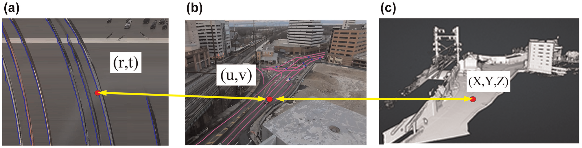
Three coordinate systems in LiDAR-Camera system using scanline method: (a) spatial-temporal map coordinates, (b) traffic video coordinates, and (c) LiDAR model coordinates.
The following part of this section will explain how to link video coordinates
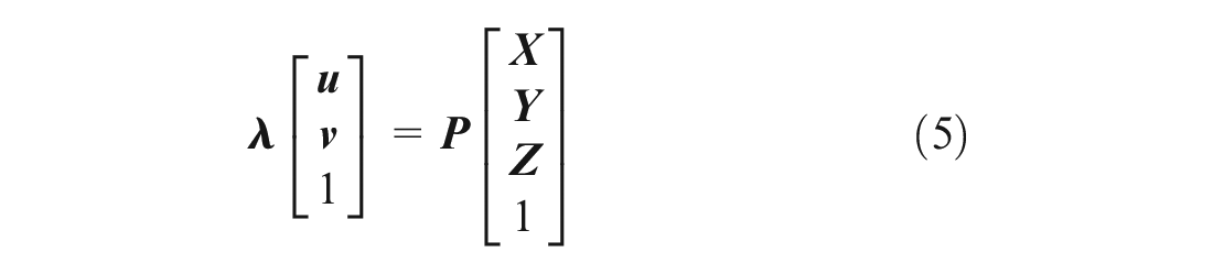
where
The intrinsic parameter can be obtained through camera calibration in the lab or from known camera model parameters. The method used to compute matrix
Equation 5 can be rewritten as Equation 6

where


Equations 7, 8 can be written as:


By rearranging the items, we obtain Equation 11 as:
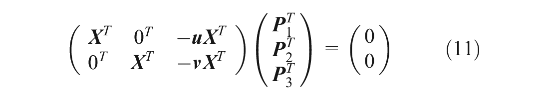
For
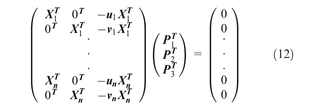
Equation 12 can be simply represented as the Equation 11

where A is a 2n * 12 matrix, which is known from 3D and 2D reference points and X is 12 by one matrix that contains all parameters in projection matrix
The problem of solving parameter in P is converted to the problem to minimize
As we know the projection matrix

where
To enforce the orthogonal property of rotation matrix

Then we obtain optimized rotation matrix


Therefore, we reconstruct the projection matrix P through the equation below.

OpenCV’s Camera Calibration and 3D Reconstruction API (Application Programming Interface) are used in this research to obtain all projection matrix parameters.
PTZ Camera Recalibration using Motion Estimation
One crucial issue for traffic monitoring is the ever-changing remote-controlled PTZ cameras. In our system, The LiDAR-Camera model mentioned above is initially well-calibrated at the time when the traffic camera is in use. To restore the 3D/2D relationships of the PTZ camera, the relative camera motion between the pre-calibrated camera and zoomed/rotated camera is identified. There are two categories of motion estimation methods, direct methods versus indirect methods. Direct methods include phase correlation, block matching, and optical flow. Indirect methods often refer to feature-based methods. In this study, the indirect method of motion estimation is used to estimate the camera movement.
Figure 15 shows the matched SIFT (scale-invariant feature transform) features ( 48 ) between a calibrated camera and a moving camera. Once the matched features are found, we can establish the coordinate system transformation between the calibrated camera image and the real-time camera using perspective transformation. Any pixel from the video frames after PTZ operations will be projected onto the pre-calibrated camera image. Therefore, the PTZ camera 2D coordinates can be transformed into 3D coordinates using the calibrated LiDAR-Camera system.
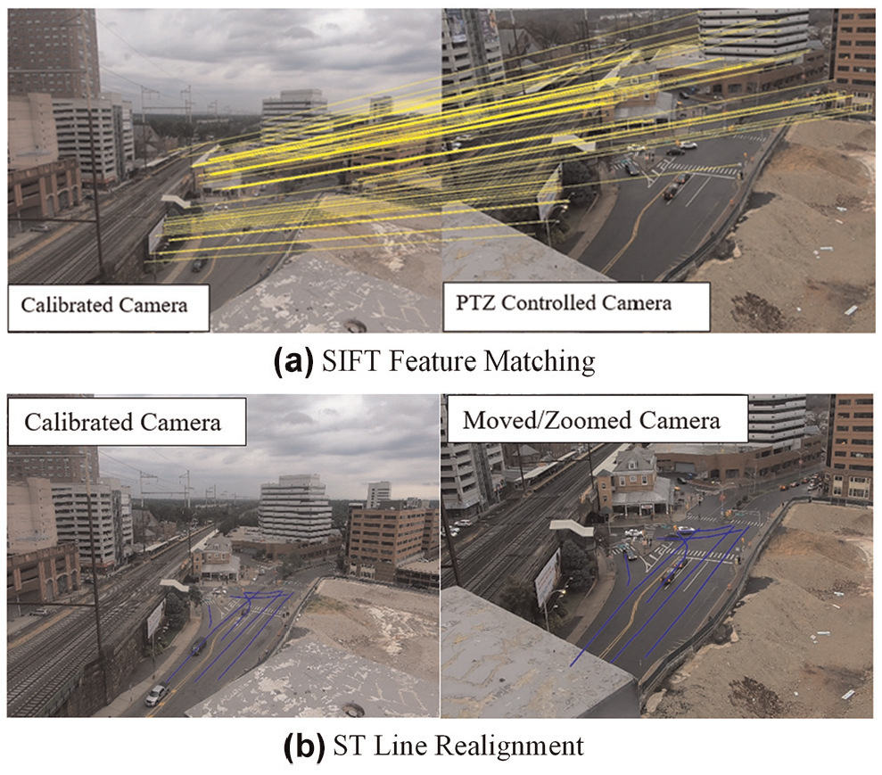
SIFT feature matching between the original image and image after PTZ operations and sample ST line recalibration results.
Multiple images from different angles will be pre-calibrated using the LiDAR model during the initial stage to cover the entire surveillance area. The pre-calibrated camera images will be used as static data. Every time the traffic operator moves the PTZ camera, the program will automatically find the best match from candidate calibrated images to build a new 2D-3D transformation. This method indirectly recalibrates the PTZ camera by matching the new camera scene with pre-calibrated photos, resulting in better accuracy and quick response.
Model Validation and Evaluation
Scanline Detection Validation and Evaluation Process
The trajectory detection results of the proposed model are validated and evaluated based on both the trajectory level and the point level. The ground-truth traffic volume data were provided through a commercial video analysis platform ( 49 ). We validated the trajectory-level performance by comparing the ground-truth traffic volume with the proposed scanline-based traffic volume at four cross-sections, as shown in Figure 16a.
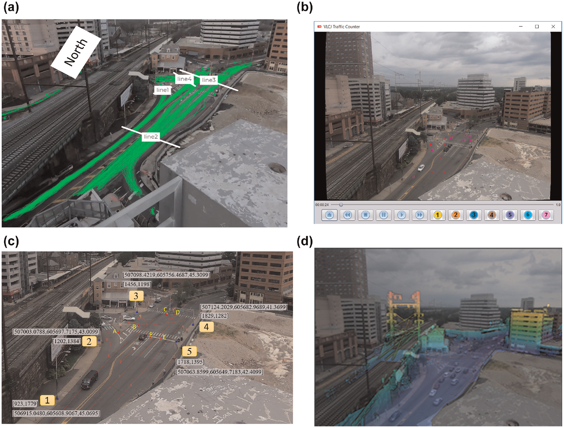
2D video detection and 3D LiDAR model validation: (a) ground-truth volume data, (b) virtual lane detector (VLD) for trajectory point validation, (c) reference points for camera calibration in both video coordinates and GPS coordinates, and (d) 2D-3D matching results.
To evaluate the point-level performance of scanline-based trajectory model, we developed a manual video counting tool with VLC (VideoLAN Client) media player API to collect the sampled video timestamps of vehicles passing some pre-determined scanline points as shown in Figure 16b. Two points were pre-defined along each scanline. One is the entry point, representing the point where vehicles are getting on the scanline. The other point is the exit point, representing the point where cars are getting off the scanline. When a vehicle hits the entry point or endpoint along its traveling direction, we click the button of the lane number on the VLC interface to record the timestamp of that event. We then compare the manually collect trajectory points with trajectory points using the proposed method to evaluate the accuracy of our proposed model.
The two-level trajectory detection results are presented in the result analysis section.
LiDAR-Camera Projection Validation
We calculated the projective transformation matrix between the LiDAR point cloud and the CCTV video by picking five key points in the study area (selected locations can be seen in Figure 16c). To quantify the performance and accuracy of the 2D-3D matching algorithm, we prepared a validation dataset consisting of six points. The pixel coordinates and GPS coordinates of each feature point in the validation set were recorded. We then applied the computed 2D-3D projection matrix to transform the 3D coordinates back to 2D pixel coordinates. We used the Mean Squared Error (MSE) to estimate the difference between the values of the projection result and the recorded pixel coordinates. The MSE for validation feature points is 1.7025 pixels given 2.7K image resolution, indicating good accuracy.
Table 1 shows the validation data, project errors, and calibrated projection parameters for this LiDAR-Camera system.
Validation of Proposed Calibration Method with Ground-Truth GPS and Photo Information
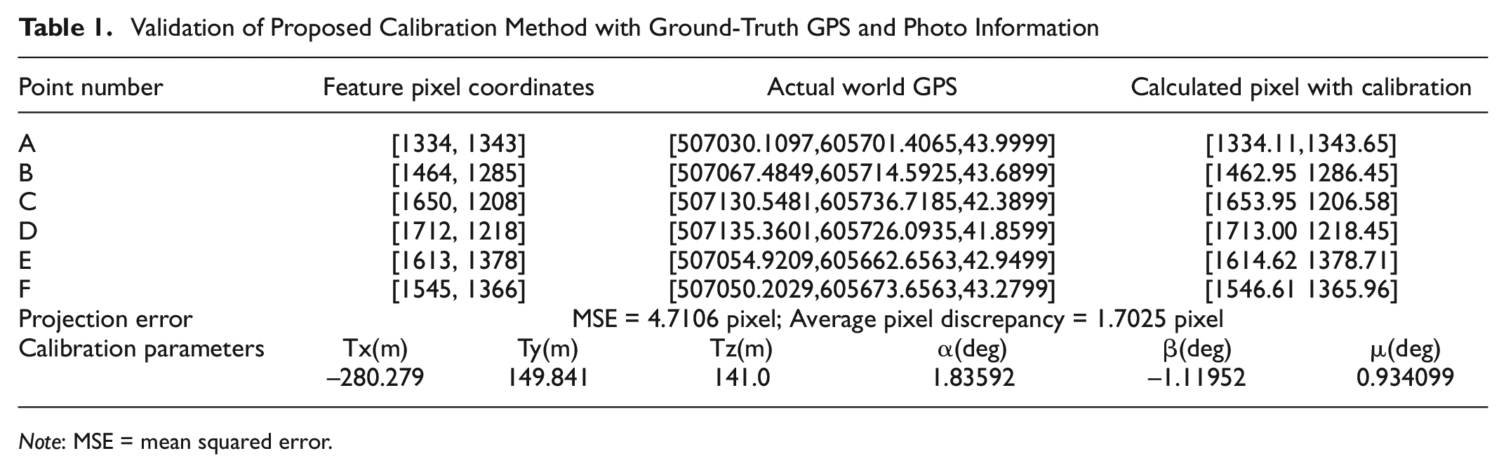
Note: MSE = mean squared error.
Study Area and Dataset
Video Data
The selected signalized intersection belongs to a small urban corridor in the city of New Brunswick in New Jersey, which has access to a major highway, transit station, university, hospitals, important company center (Johnson & Johnson headquarters), and planned innovation hub buildings. The testing video was taken during the afternoon peak (4:30–5:00 pm) on Monday, February 17, 2020. The camera was set up on the rooftop of the 10th-floor parking garage with approximately 45° angle toward the intersection. By zooming in to the intersection, the video mimics a typical roadside CCTV traffic camera view.
LiDAR Data
LiDAR data were obtained by the Rutgers MLS, as shown in Figure 13. The Velodyne LiDAR HDL-32E was used in this case study. It has 32 channels and can collect around 1.39 million points per second while maintaining a precision accuracy of ±2 cm. The LiDAR data collection range is between 80 m and 100 m. Mobile LiDAR data for New Brunswick downtown were collected on 02/17/2018. The test site (40.496326 N and –74.446131 W) is close to New Brunswick Train Station along Albany Street, which is one of the busiest streets in relation to traffic volume in the city of New Brunswick.
Result Analysis
In this section, we will discuss the scanline-based vehicle trajectory detection result, present projected physical trajectory with a 3D LiDAR road map, and demonstrate the potential benefits of using LiDAR-assisted video traffic analysis.
Scanline-based vehicle trajectory detection results (Table 2) show the detected vehicle data and ground-truth data at both trajectory level and point level. The total volume detection accuracy is 90.87% for all four main approaches. Because of the tilted camera angle, the scanline on one lane might capture vehicles from the adjacent lane. The invasions of adjacent-lane vehicles lead to duplicated counts of vehicle volume. A potential solution to remove duplicated counts is to find the concurrent detections on adjacent lanes.
Scanline Vehicle Detection Validation Results

The second half of Table 2 shows the point-level trajectory detection results by comparing manually extracted points with the model trajectory. An event is defined as a vehicle hitting either the enter point or the exit point on the scanline. The timestamps were recorded when we observed a vehicle passing through the virtual lane detector on the video. The average detection rate for point-level validation is 88.09%. In Figure 17, most of the sampled points are aligned with the trajectory outputs, which indicates a good model performance for trajectory detection.
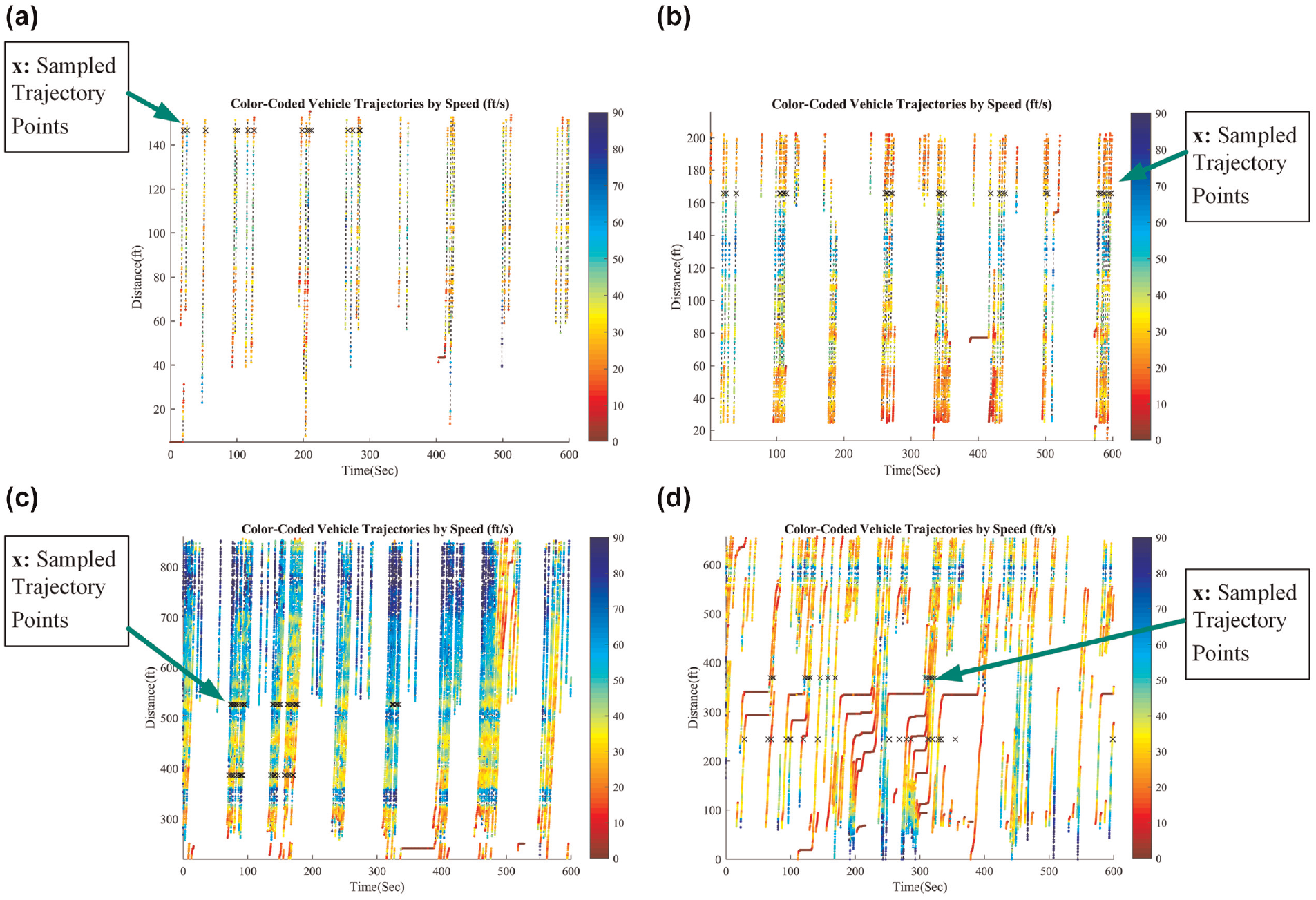
Color-coded vehicle trajectory for major directions: (a) southbound right turn, (b) southbound left turn, (c) westbound through, and (d) eastbound through.
LiDAR-Camera Projection
Figure 17, a–d , shows the detected trajectories based on travel distance along the scanline, including four major directions for eight signal cycles in 10 min. The trajectories are color coded, where red indicates a slower speed, and blue indicates a faster speed. The black crossings are sampled trajectory points using a virtual video counter to validate the model at the point level.
In Figure 18, one cycle of trajectory data is presented to provide the close inspection of model results. To better illustrate how the trajectory on the ST Map is converted into a physical trajectory. We provide the ST Map trajectory picture in Figure 18e. As shown in Figure 18, d and e , the physical trajectories are consistent with the vehicle movement captured by the ST Map. Some issues can be identified by comparing the pixel trajectory with the physical trajectory. The vehicle trajectories at the bottom of the ST Map are not detected efficiently. Because those vehicles are too far from our camera, they overlap together on the ST Map. In future improvement, the remaining textures in these occluded areas, especially those line features will be further explored.
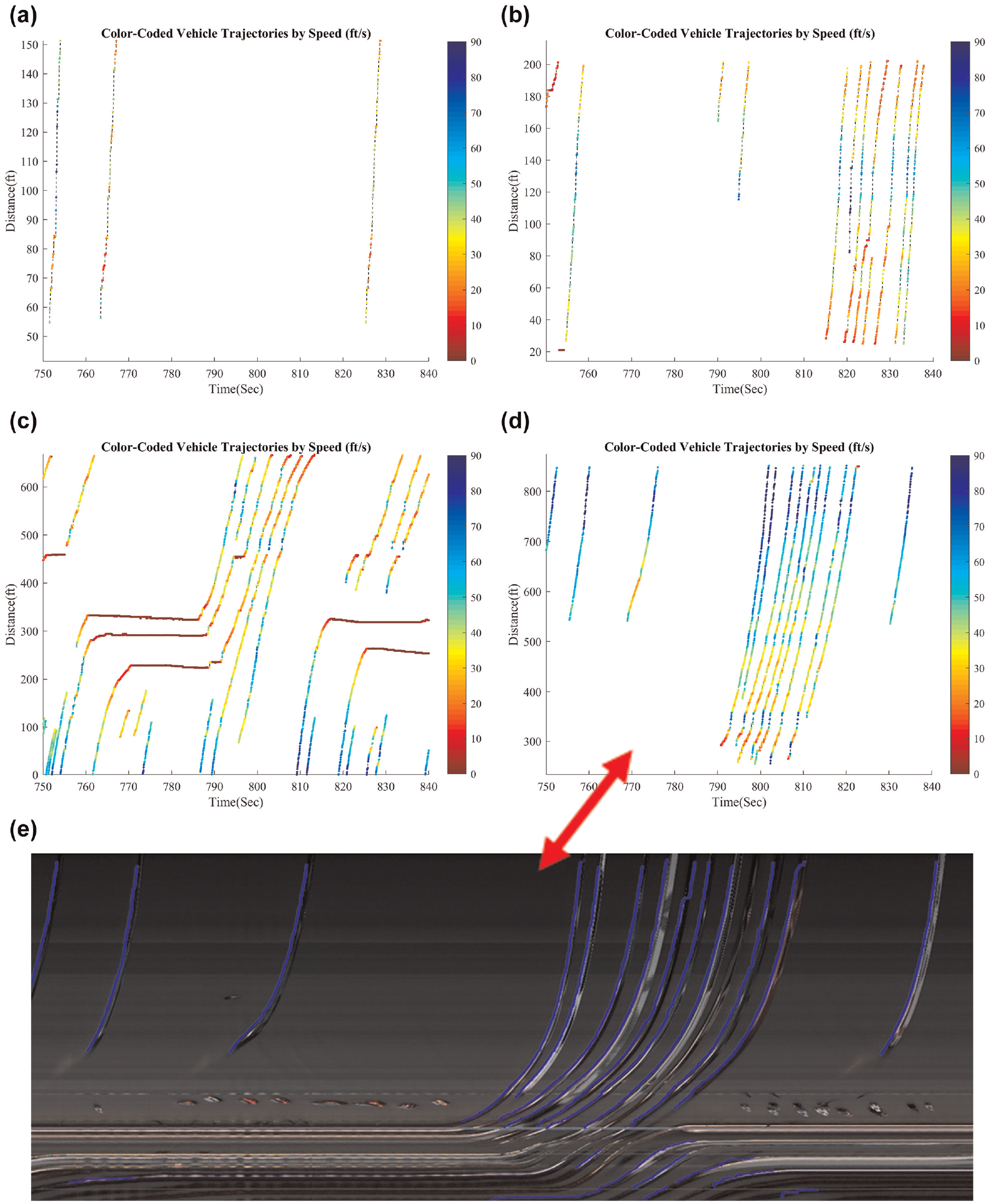
Examples of miss detection because of severe occlusions within one signal cycle: (a) southbound right turn, (b) southbound left turn, (c) eastbound through, (d) westbound through, and (e) westbound through trajectory on the ST Map.
Figure 19 illustrates the physical trajectory projected on the 3D urban infrastructure map by using the 3D/2D mapping method. This picture demonstrates many more prominent features using the LiDAR system than other camera calibration models. With the growth of large-scale digital mapping systems, we can acquire more and more realistic and extensible trajectory data using the proposed system to build traffic flow profiles and promote various traffic studies.
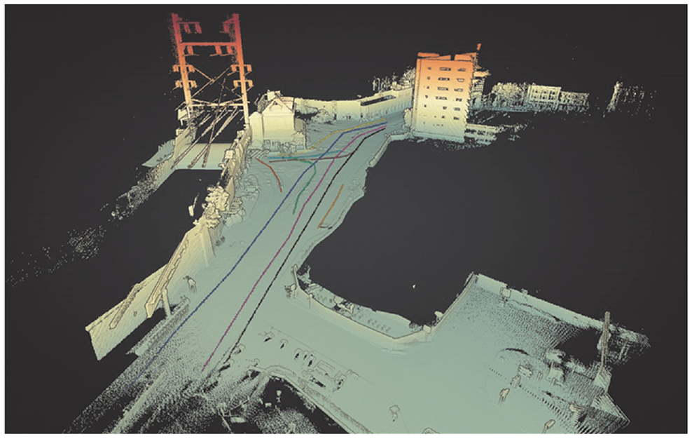
Sample projected physical trajectories on high-resolution 3D street model.
Trajectory-Based Traffic Performance Measurement
Figure 20 is the illustration of two performance metrics that can be used as intersection performance measurements for operational analysis. Figure 20a is the frequency heat map that shows the frequencies of detected vehicles. The brighter areas indicate the higher detected vehicle frequency, implying a queuing/congestion issue, long waiting time, and limited capacity. As we can see, the waiting time for the westbound lane is the highest, which is consistent with our observation from the video. This detection frequency map can be used to diagnose traffic congestion to accommodate fluctuated traffic.
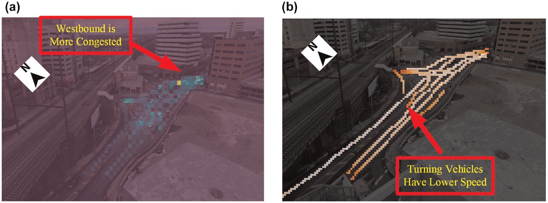
Traffic analysis using scanline detection and LiDAR-assisted calibration: (a) detection frequency heat map, and (b) intersection speed heat map.
Figure 20b is created after calculating the moving speed of each object using the GPS position of each trajectory point. The average speed heat map is a useful performance metric for intersection safety management, because of many crashes being speed-related. Speed profile is critical to optimize signalized intersection based on traffic flow theory, as there is a fundamental relationship between speed, queue, and volume. However, without LiDAR assistance, it is usually too difficult to know the real-world speed characteristic of traveling vehicles from just CCTV cameras.
In the future, CAV technology such as Eco-intersection Approach and Intelligent Signal Control will lead to more harmonized speed characteristics. The performance metrics generated from trajectory data are critical for CAV-based traffic operation, as they can provide proactive solutions and depict a better picture of the traffic network.
Conclusion
Different from conventional detector data, trajectory-based traffic data often provide greater detail and flexibility when generating various types of performance measure data for traffic operations and management. However, real-time operational systems require accurate but computationally efficient algorithms that can generate vehicle trajectories in real-time with conventional CCTV traffic camera systems.
The proposed Longitudinal Scanline LiDAR-Camera (LSLC) model has been built with significant improvement to address the challenges brought by the complex road surface, occlusion, noise because of hanging wires, lane markings, control devices, stopping, and crossing traffic. An adaptive background subtraction algorithm is introduced to eliminate noises on ST Maps caused by multi-color road surfaces, line blockages by intersection control devices, wiring, and lane markings. A suite of processing modules, including connected component filtering and zigzagging removals, is proposed to significantly improve the quality of the results. A proposed recalibration algorithm further allows the proposed model to quickly realign ST lines and re-project vehicle coordinates after PTZ operations by estimating the camera motion using the automatic SIFT feature matching algorithm.
The 3D point cloud collected from static LiDAR scanning is used to build a clean 3D infrastructure model of the arterial infrastructure. The resulting 3D model can then be used to establish the 2D-3D transformation model to convert pixels in the video frame and their physical points in the 3D model to generate vehicle trajectories in world coordinates. Compared with previous traffic camera calibration methods, the LiDAR-assisted traffic video analysis method does not rely on VP detection, reference objects, or statistic assumptions about average speed or vehicle dimensions. The proposed model turns the ubiquitous CCTV traffic camera into a high-fidelity data source that can facilitate innovative traffic management and a variety of CAV applications in the future.
Future work in this study includes the further exploration of computer vision algorithms that can deal with severe occlusions among remote pixels and other potential computer vision noise caused by weather, illumination, and heavy vehicles. Furthermore, it is crucial to study the scaling of the proposed applications to large arterial networks through cloud computing platforms.
Footnotes
Acknowledgements
Special thanks to Middlesex County, The City of New Brunswick, and New Brunswick Parking Authority for assistance in data collection. We would like to thank GoodVision for providing the trial credits for generating the comparison data.
Author Contributions
The authors confirm contribution to the paper as follows: study conception and design: Peter Jin, Tianya Zhang, and Jie Gong; data collection: Peter Jin, Jie Gong, Tianya Zhang, Yi Ge, and Mengyang Guo; analysis and interpretation of results: Tianya Zhang, Yi Ge, and Mengyang Guo; draft manuscript preparation: Tianya Zhang, Mengyang Guo, and Peter Jin. All authors reviewed the results and approved the final version of the manuscript.
Declaration of Conflicting Interests
The author(s) declared no potential conflicts of interest with respect to the research, authorship, and/or publication of this article.
Funding
The author(s) disclosed receipt of the following financial support for the research, authorship, and/or publication of this article: This work was partially funded by NSF IIP-1827505: PFI-RP: Smart and Accessible Transportation Hub for Assistive Navigation and Facility Management. The research was partially supported by NSFC (National Science Foundation of China, Grant No. 61620106002).
Data Accessibility Statement
The traffic videos, intersection LiDAR, and trajectory detection results datasets can be provided on request by contacting the corresponding author, Dr. Peter J. Jin, at