
Abstract
Weaving segments are among the most important segments in any kind of facility. One of their key features is their maximum length (Lwmax), which determines the performance of the facility as a weaving or separate merge and diverge segments. Based on an equation in the Highway Capacity Manual (HCM 2016), only two variables VR (volume ratio) and Nwl (number of weaving lanes) influence this length. However, certain cases can be found in which traffic conditions are different but Nwl and VR values are equal. In this study, three separate weaving segments in Tehran, Iran were used and their data were collected to further analyze the influence of the traffic parameters. Calibration of field data was performed using GEH values of freeways and ramps for simulation and field traffic volumes. The simulation was therefore used on the basis of different traffic and geometric parameters, and the effects of these parameters on Lwmax were carefully observed. There were 184 simulated scenarios in Aimsun using data collected from the three weaving segments in Tehran plus simulation. In these scenarios, two geometric parameters (Nwl and Lwmax) and four traffic parameters were considered variable. It was found that for Nwl = 2 the accepted regression model containing three new variables has an R2 value equal to 0.95, and for Nwl = 3 two of the three variables were used for the model produced with an R2 value equal to 0.7.
According to the Highway Capacity Manual (HCM 2016), weaving is generally defined as the crossing of two or more traffic streams traveling in the same direction along a significant length of highway without the aid of traffic control devices (except for guide signs). Thus, weaving segments are formed when merge segments are closely followed by diverge segments. “Closely” implies that there is not sufficient distance between the merge and diverge segments for them to operate independently ( 1 ). Weaving segments have a variety of significant characteristics. One of them is their maximum length, which determines the type of performance of the segment. If the short length (Ls) is less than the maximum length (Lwmax), it operates as a weaving segment, otherwise it is a merge and a diverge segment. According to HCM, the analysis of the segment is based on the type of performance and is different.
In HCM, there is an equation for calculating the maximum length of the weaving segment, written below:

where Lwmax is the maximum weaving length, VR is the ratio of weaving volume to total volume of traffic, and Nwl is the number of lanes from which a weaving maneuver may be made with one or no lane changes.
The maximum weaving length depends on only two variables according to the equation1: VR (volume ratio) and Nwl (number of weaving lanes). If these two variables are constant, the maximum weaving length will also be constant. However, in the case of a weaving segment with a particular geometry (Nwl is constant), a situation may be assumed in which VR is constant, but the volume of traffic varies with the passage of time. In this case, according to Equation 1, maximum weaving length will not be changed, which does not make sense, as traffic volumes have been changed.
The only traffic variable to obtain Lwmax in HCM is VR. In this study, therefore, it was attempted to define new traffic variables describing the conditions of the weaving of traffic and to generate a model to calculate Lwmax based on these variables. New variables define the intensity of weaving traffic more precisely than VR and also include traffic volumes in themselves.
Literature Review
Traffic in weaving segments has been studied by data analysis. Using vehicle counts from loop detectors in two separate weaving areas in the United States, Cassidy and Lee and Skabardonis and Kim showed that disruptive lane changes from ramp to freeway could cause the activation of bottleneck ( 2 , 3 ). The results of the lane changing in the weaving lane are further analyzed in Rudjanakanoknad and Akaravorakulchai with video data collected in a Bangkok weaving segment ( 4 ). The researchers show that the capacity of the studied weaving segment fluctuates over time depending on the number and destination of changes in the lane. They noted that raising on-ramp demand contributes to lane changes from slow to fast lanes, thereby increasing overall capacity. They also pointed out that an increase in demand for off-ramps results in lane-changing rates from fast to slow lanes and reduces the capacity of the studied weaving segment.
Turbulence is a major problem that exists in weaving segments. In the vicinity of motorway ramps, drivers entering the motorway, leaving the motorway, and cooperating or anticipating on entering or exiting vehicles perform multiple maneuvers. Such maneuvers include lane changes, speed, and headway changes. This leads to changes in the lane flow distribution, higher speed variation, and changes in the headway distribution of the different lanes, with a possibly higher proportion of small gaps on the outside lane ( 5 , 6 ). This phenomenon is referred to as turbulence in the literature and the guidelines for the design of motorways. A higher turbulence level around motorway ramps is expected ( 7 , 8 ) and has a negative impact on the capacity and safety of the motorway ( 8 – 14 ).
The literature and design guidelines conclude that an increased turbulence level is present upstream and downstream of a ramp. This zone is referred to as the area of ramp influence ( 8 ) and specifies the ramp spacing required to avoid traffic and traffic safety disturbances. The turbulence level was shown to increase upstream and decrease downstream of a ramp. However, when it comes to the length of this area of influence there is no consistency ( 7 ). There are only two empirical studies available to the best of our knowledge that show the limits of the area of ramp influence. Kondyli and Elefteriadou studied instrumented vehicle observations and found that the area of influence of the ramp begins at 110 m upstream and finishes at 260 m downstream of the gore of a ramp ( 11 ). Van Beinum et al. studied loop detector data from multiple ramps and found that the ramp influence area begins upstream at 200 m (on-ramp) or 900 m (off-ramp) and ends downstream of the ramp gore at 900 m (on-ramp) ( 6 ). It was recommended that the turbulence influence length of individual vehicles should be analyzed in future research using empirical trajectory data.
Whether it is a weaving or an isolated (merging or diverging) segment, understanding the length of the weaving segment will determine the nature of the segment’s traffic operations. The HCM 2000 edition sets the maximum weaving segment length for Type A at 600 m and for Type B and Type C at 750 m ( 15 ). A weaving segment with a length greater than these limits is therefore considered to be a separate on-ramp followed by an off-ramp. Although HCM 2000 used a constant value of 2500 ft (762 m) for the maximum length, HCM 2010 used a variable value. This length is also considered variable in HCM 2016. Specification of the appropriate value was based on traffic volumes and configuration characteristics.
Most lane changes occur within the first 150 m of the weaving area between the ramp and the motorway ( 16 , 17 ). Such findings were derived from the study of a large amount of empirical and simulated data from several sites around California, U.S.A. Stewart et al. reported that if the distance between the on and off-ramp is less than 300 m, this would create more turbulence ( 18 ). Wang et al. found that the length of the weaving segment had different impacts under different weaving configurations on the capacity of general traffic ( 19 ), whereas Shoraka and Puan reported that for the two lanes adjacent to the merge gore, the first 75 m from the entrance point had the highest rate of lane changing and the highest concentration of flow ( 20 ).
Some research on the length of the weaving segment has been done. In Grenoble, France, Marczak et al. studied empirical trajectory data from a segment of urban motorway weaving. They found that only 60% of the total length of the weaving segment is used for weaving under free-flow conditions, leaving 40% of its length unused ( 21 ). They also found that vehicles from the acceleration/deceleration lane to the main road accept smaller gaps than vehicles from the main road to the acceleration/deceleration lane. The researchers conclude that the length of a weaving segment may not be significant in the capacity estimate. Kusuma et al. analyzed trajectory data from video recordings in combination with traffic flows and loop detector speeds in the United Kingdom and found that 91% of traffic decelerates at the beginning of the weaving segment to cooperate with merging and diverging traffic, and 48% of lane-changing vehicles change lanes in the first 25% of the weaving segment ( 22 ).
Modeling Approach
In this study, using three weaving segments in Tehran, Iran, and keeping the basic geometry of these segments unchanged, the lengths of them have been increased to 2,000 m and more. Simulation was done for separate traffic situations in Aimsun software by assuming different traffic volumes for Nwl = 2 and 3. In certain traffic cases, the value of the VR was kept constant. Field data on West Hakim, North and South Yadegare Emam highways in Tehran were collected from three weaving segments on these highways. Data collection took place on the weekday of October 13, 2018, when the usual conditions (normal weather conditions, no incident and working zone upstream and downstream of weaving segments) were expected to occur. Calibration of the simulation model is done on the basis of these field data.
By using field data and simulation, two new regression models have been developed for Nwl = 2 and 3. Three new variables including FR (
Methodology
Three weaving segments in Tehran, Iran were assumed to obtain new equations for maximum weaving segment length with new variables. By increasing the maximum length of these segments to 2000 m and more and also maintaining a constant VR amount in some traffic scenarios used and simulated in Aimsun software, Lwmax values are obtained in all traffic scenarios under Nwl = 2 and 3 circumstances. In Nwl = 2, the highway has three lanes before on-ramp and after off-ramp and four lanes in the segment of weaving, and both ramps have only one lane. But there are two lanes in Nwl = 3 before the on-ramp, four lanes in the segment of weaving and three lanes after the off-ramp. Both ramps have two lanes. The free-flow speed (FFS) is also equal to 80 km/h on the highway before the on-ramp and after the off-ramp. In the weaving segment on the two most right-hand lanes, the FFS is equal to 60 km/h, in the third lane it is 70 km/h, and in the left-most lane it is equal to 80 km/h. In the on-ramp and off-ramp, FFS is equal to 50 km/h.
It is better to provide a summary of the scenario development in Aimsun. Each scenario defined in Aimsun has an origin–destination (O-D) traffic volume matrix of all four maneuvers in a weaving segment. In this study, for Nwl = 2, for each VR number, 6–8 and for Nwl = 3, 13 scenarios or O-D matrices were added to the software. After entering traffic volumes for each scenario, a traffic demand has been defined that includes the relevant O-D matrix. It is obvious that the number of traffic demands should be the same as the scenarios or matrices.
In the final stages of the simulation a dynamic scenario is created, and then an experiment is made in Aimsun. In this part, by choosing the type of simulation (microscopic, mesoscopic, or hybrid simulator), then by determining the number of replications (the number of analyses performed by the software), and finally by assigning traffic demands to the specified experiment, simulation (running each replication) will begin.
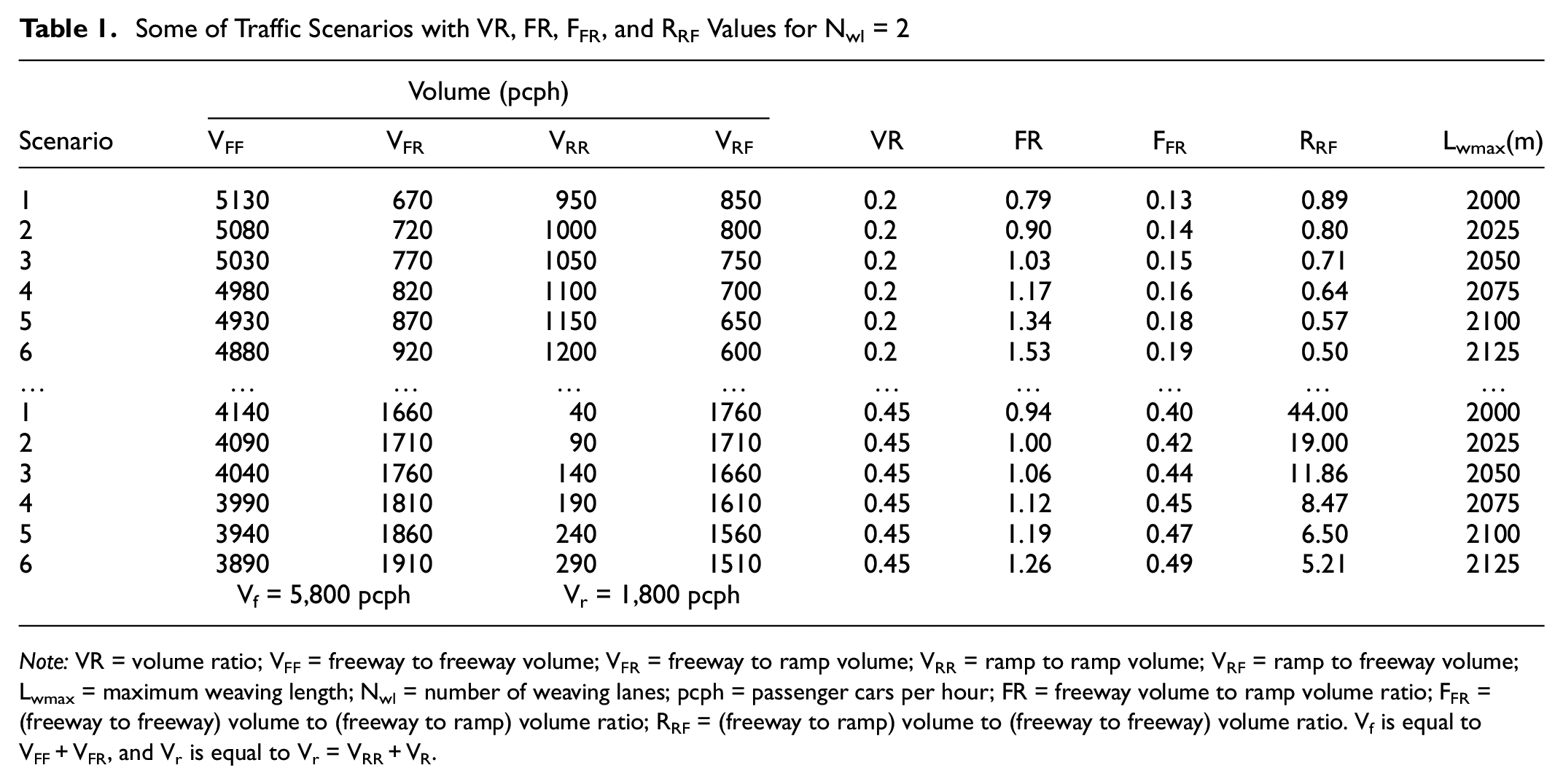
It should be noted that these weaving segments perform under capacity conditions (traffic flow equal to capacity) in such a way that the weaving length values obtained from the simulation are equal to the maximum length. The simulation capacity of each lane is equal to 2000 passenger cars per hour (pcph) based on FFS and some HCM tables. Every lane is 3.5 m wide. Some of traffic scenarios are shown in Tables 1 and 2 with their VR, FR, FFR, and RRF values for Nwl = 2 and 3. Traffic volumes are in passenger cars per hour in these tables and Lwmax values are in meters. Index F refers to the freeway in traffic volumes and R refers to the ramps. The parameters mentioned are defined as follows:
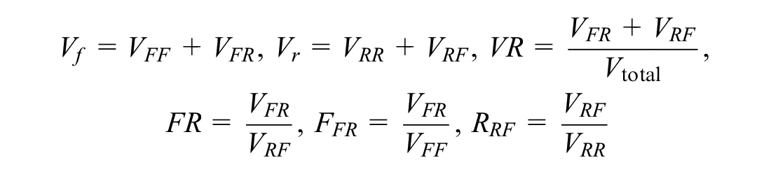
Some of Traffic Scenarios with VR, FR, FFR, and RRF Values for Nwl = 2
Note: VR = volume ratio; VFF = freeway to freeway volume; VFR = freeway to ramp volume; VRR = ramp to ramp volume; VRF = ramp to freeway volume; Lwmax = maximum weaving length; Nwl = number of weaving lanes; pcph = passenger cars per hour; FR = freeway volume to ramp volume ratio; FFR = (freeway to freeway) volume to (freeway to ramp) volume ratio; RRF = (freeway to ramp) volume to (freeway to freeway) volume ratio. Vf is equal to VFF + VFR, and Vr is equal to Vr = VRR + VR.
Some of Traffic Scenarios with VR, FR, FFR, and RRF Values for Nwl = 3
Note: VR = volume ratio; VFF = freeway to freeway volume; VFR = freeway to ramp volume; VRR = ramp to ramp volume; VRF = ramp to freeway volume; Lwmax = maximum weaving length; Nwl = number of weaving lanes; pcph = passenger cars per hour; FR = freeway volume to ramp volume ratio; FFR = (freeway to freeway) volume to (freeway to ramp) volume ratio; RRF = (freeway to ramp) volume to (freeway to freeway) volume ratio. Vf is equal to VFF+VFR, and Vr is equal to Vr = VRR + VRF.
As can be seen from Tables 1 and 2, maximum weaving segment length increased by raising FR and FFR and decreasing RRF for each particular value of VR. This means that in a certain amount of Nwl, Lwmax has a direct relationship with FR and FFR and an indirect relationship with RRF.
Data Collection
Field data on West Hakim, North Yadegare Emam, and South Yadegare Emam highway in Tehran, Iran were collected from three weaving segments on the cloverleaf of Hakim and Yadegare Emam highways (Figure 1). These highways are classified as two principal urban arterials with a speed limit of 80 km/h based on the AASHTO classification system ( 23 ). Lateral clearance equals to 85 cm for Hakim Highway and 50 cm for Yadegare Emam. Weaving segment length is 153 m for West Hakim Highway, 178.5 m for North Yadegare Emam, and 91.2 m for South Yadegar. There are three lanes before the on-ramp and after the off-ramp in all three weaving segments mentioned above and four lanes within the weaving segment, and the auxiliary lane is wider than the other three lanes. For all sites, on-ramps as well as off-ramps have only one lane equal to nearly 7 m wide.

Location of three studied weaving segments (attribution information: 35°44′26.49′′ N, 51°20′49.24′′ E, elevation: 4,449 ft, eye alt: 6,390 ft).
Data collection took place on the weekday of October 13, 2018, when the regular conditions (normal weather conditions, no incident and work zone upstream and downstream of weaving segments) were assumed to occur. Data were collected in two periods of 2 h: 6:30–8:30 a.m. and 3:00–5:00 p.m., which are the peaks of the weaving segments and the volumes of traffic in those periods equal to almost the capacity of the weaving segment. The data are collected at intervals of 5 min and then aggregated at intervals of 15 min.
Collected data include traffic volumes of different maneuvers, origin destinations (ods), aggregate speed of all vehicles (including passenger cars and heavy vehicles), and geometric data of the weaving segments. The data collection consisted of counting the number of vehicles on the plate and filming (using a camera) the above-mentioned weaving segments. Figure 1 (taken from Google Earth) shows the location of three segments of weaving studied in this research.
Calibration
There are many studies on the calibration of traffic simulation models. You may refer to Hourdakis et al. ( 24 ) as an example of how Aimsun is used as a micro simulation tool for a freeway. Volume was the performance output of this study. The data used in the calibration process were also 5-min data from 21 detector stations for a 12-mile freeway section during p.m. peak for 3 days.
As can be seen from the above study, peak periods are not more than a few days. The data therefore only record a few specific conditions, or are a diluted selection of different conditions. So, the model predictions are assumed to be correct only for those special conditions.
In recent years, significant attention has been paid to the effects of data and parameter uncertainty on traffic simulation models ( 25 , 26 ). Research from other fields shows that bias and variance in simulation output results are caused by bias and variance in input models used after simulation error that has been eliminated; input models include inputs and simulation model parameters ( 27 , 28 ).
In this study, a microscopic traffic simulation model was developed for the three studied weaving segments using Aimsun software. Based on the FFS of 80 km/h (50 mi/h) in all three weaving segments studied in this research, the capacity is equal to 2000 passenger cars per hour per lane (pcphpl) according to HCM 2016 exhibit 12-4. On-ramp and off-ramp capacity was determined in accordance with HCM 2016 exhibit 14-12. The capacity of each ramp is equal to 1900 pcph based on FFS = 40 km/h (25 mph) and for single-lane ramps. According to the explanation above, the capacity values for each lane are entered in Aimsun at the calibration step.
After setting up the required simulation elements, the weaving segment calibration was performed. This step is performed for traffic volumes. Real traffic volumes (field condition) of three weaving segments were entered in the simulation to observe the flow of each segment and compare it with field conditions. If there was a big difference between field and simulated flow, the traffic condition in the simulation network would not reflect the actual network and the simulation tests would not be valid. The network can only be used for further applications, such as safety improvement and efficiency tests, after a satisfactory calibration of the simulation network has been carried out.
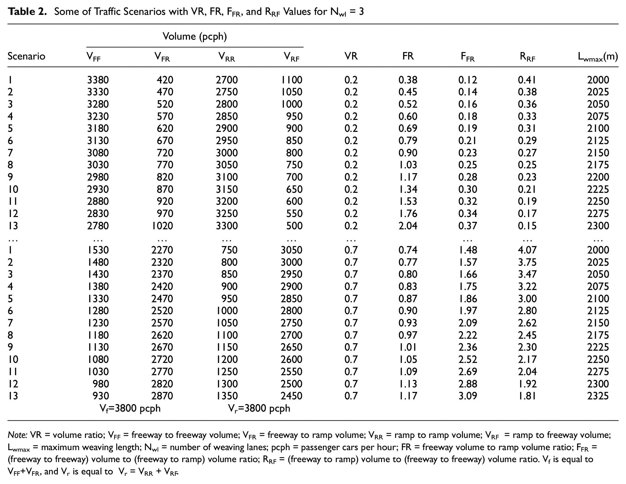
The Geoffrey E. Havers (GEH) Statistic was computed by comparing simulated volume and field volume to calibrate the simulated network ( 29 ). GEH is defined as Equation 2.

where E is simulated volume (vehicles per hour) and V is field volume (vehicles per hour). If more than 85% of the GEH values of the measurement locations are below 5, the simulated volume will accurately reflect the field volume ( 30 ).
Three weaving segments were calibrated for this study. Seven 15-min intervals are specified to be calibrated for each of these segments. Segments of weaving and on-ramps are determined to calculate their GEH value. The average flow amounts of three simulated replications in Aimsun are determined as the Aimsun simulation volume for each time interval in Table 3. The time intervals chosen for Table 3 are the most crowded, carrying the highest number of vehicles in the three weaving segments analyzed in this study. Table 3 shows GEH values for three weaving segments and on-ramps. The table shows a good calibration of these segments. Just two of the 21 GEH measurements are greater than 5.0, with GEH values greater than 5 for the weaving segment only and appropriate GEH values for the on-ramps. Thus, 90.5% of the GEH value of the observations was less than 5.
Weaving Segment GEH Values for Calibration
Note: GEH = Geoffrey E. Havers; Abs(Dif) = absolute difference; F-vol = field volume; A-vol = Aimsun simulation volume. Bold indicates a value greater than 5 (allowable GEH value).
Modeling and Results
Linear regression is a useful tool for predicting a quantitative response. Linear regression has been around for a long time and is the topic of innumerable textbooks. Though it may seem somewhat dull compared with some of the more modern statistical learning approaches, linear regression is still a useful and widely used statistical learning method ( 31 ). The regression approach is used in this study because of its simplicity and interpretability.
Before starting modeling for Nwl = 2 and Nwl = 3, it is useful to see the correlation between all the important variables (including those used in modeling for Nwl = 2 and Nwl = 3) in all data for Nwl = 2 and 3. As a consequence, Figure 2 is shown below.
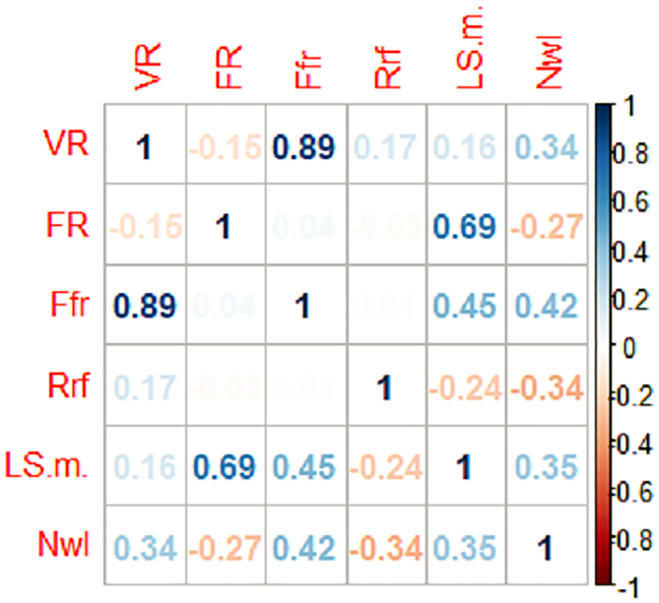
Corrplot of variables for Nwl = 2 and 3 data.
As shown in Figure 2, RRF and FFR do not have a substantial correlation with each other and can therefore be used together in a model. However, FFR has a strong correlation with VR, which means that they cannot be used together in the Nwl = 2 or 3 model. Also, FR has no high correlation with FFR and RRF, which makes sense, as FR reflects the weaving intensity of both freeways and ramps, whereas FFR and RRF reflect only the weaving intensity of freeways or ramps. FR can therefore be used together in a model with FFR and RRF.
Using field data and simulation, regression models for Nwl = 2 and 3 have been developed in R software. The first case relates to Nwl = 2. In this case, data from 41 simulated scenarios were used to generate models. The results of modeling for this case are shown in Table 4.
Summary of Regression Model Results for Nwl = 2

Note: Nwl = number of weaving lanes; FR = freeway volume to ramp volume ratio; FFR = (freeway to freeway) volume to (freeway to ramp) volume ratio; RRF = (freeway to ramp) volume to (freeway to freeway) volume ratio.
The qualitative significance level of the coefficients which relies on p-value.
Based on Table 4, there is only one model for Nwl = 2, because of the disallowed p-values of other models, as well as the presence of correlated variables in the same models. These models were omitted from Table 4. This model has accepted p-values, and high enough R2 and F-statistic amounts, so it will be chosen to calculate maximum weaving segment length values for Nwl = 2. The Lwmax equation (in meters) for this case is as follows:

In addition, statistical tests such as residual normality and homoscedasticity should be checked to accept the above model. For the first, the Shapiro–Wilk test, and for the second, the Breusch–Pagan test was performed in R.
The Shapiro–Wilk test for normality is one of three general normality tests designed to detect all departures from normality. It is comparable in power to the other two tests. The test rejects the hypothesis of normality when the p-value is less than or equal to 0.05. Failing the normality test allows us to state with 95% confidence the data does not fit the normal distribution. Passing the normality test only allows us to state no significant departure from normality was found. The result of this test for model 1 in Table 4 is shown below:

According to the above results, the p-value is more than 0.05, which means that the data used to produce Model 1 for Nwl = 2 come from a normal distribution.
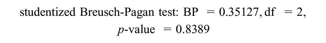
The second test is Breusch–Pagan. The Breusch–Pagan–Godfrey Test (sometimes shortened to the Breusch–Pagan test) is a test for heteroscedasticity of regression errors. Heteroscedasticity means “differently scattered;” this is opposite to homoscedasticity, which means “same scatter.” Homoscedasticity in regression is an important assumption; if the assumption is violated, we would not be able to use regression analysis. If the test statistic has a p-value below the appropriate threshold (e.g., p < 0.05) then the null hypothesis of homoscedasticity is rejected and heteroscedasticity is assumed ( 32 – 34 ). The results of this test for Model 1 are shown below:

Based on the results, the p-value is more than 0.05, which means that the Model 1 assumption of homoscedasticity is accepted.
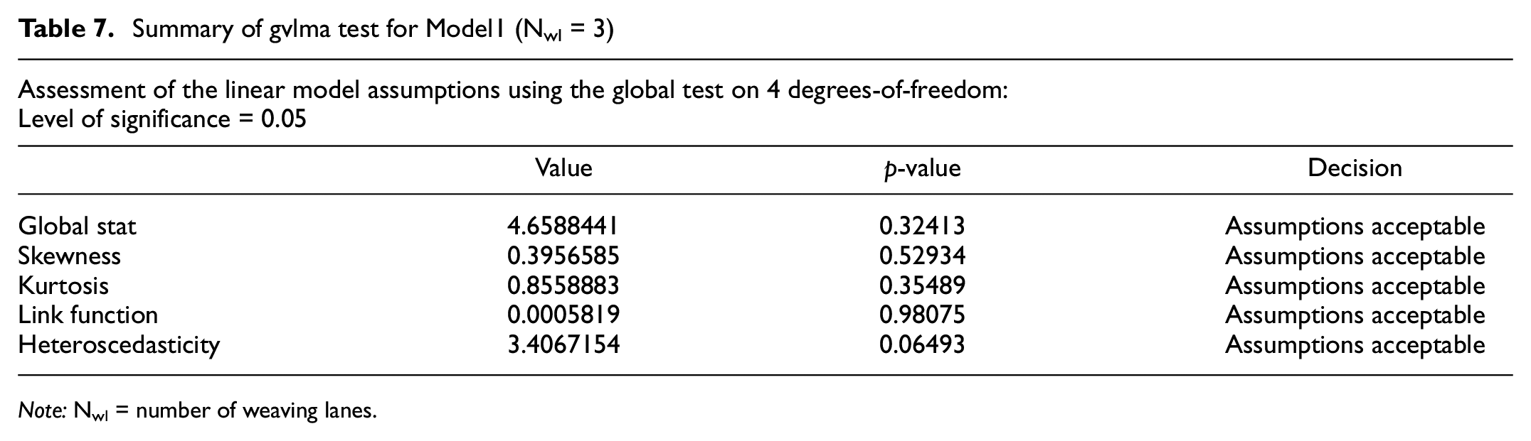
In addition, a package called “gvlma” has been used for accepted models. “Gvlma” is the abbreviation of Global Validation of Linear Model Assumptions. It is a single global test to assess linear model assumptions, as well as to perform specific directional tests designed to detect skewness, kurtosis, nonlinear link function, and heteroscedasticity. In this research, these assumptions for the linear models in the gvlma test were found on the basis of a paper dealing with the procedure for testing those assumptions for the linear model ( 35 ). The results of this test for Model 1 are shown below in Table 5.
Summary of gvlma Test for Model 1 (Nwl = 2)
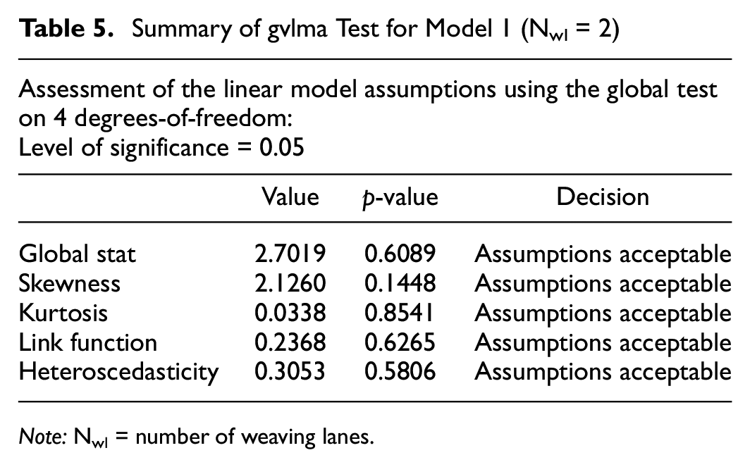
Note: Nwl = number of weaving lanes.
As can be seen from the table, the “Global Stat” (Global Statistic), which is a function of the residual model, consists of four asymptotically independent statistics, each with the potential to detect a particular violation ( 35 ). According to Table 5, all assumptions have been accepted, so there is no particular violation of Model 1.
At the end of this case (Nwl = 2), the Lwmax values obtained from the HCM equation and Model 1 are compared with each other in Figure 3.
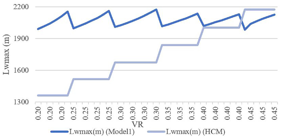
Comparison of HCM and Model 1 Lwmax values.
Figure 3 shows the trends in maximum weaving length values obtained from the HCM equation and Model 1 for Nwl = 2. As is evident, HCM is following an upward step trend, with high variations ranging from almost 1,300 to 2,200 m. Model 1 has a growing and declining pattern with a range of variations equal to 300 m. The step pattern of HCM is caused by the change of its only variable VR (Nwl is constant = 2), whereas in Model 1 the special value of VR is not constant as a result of its variables (FR, FFR, and RRF) which change over a constant value of VR. This topic shows that there should be several other variables that influence the value of Lwmax in the constant values of VR and Nwl. Also, the smaller range of Model 1 change compared with HCM indicates that Model 1 is more accurate in calculating the maximum weaving length value.
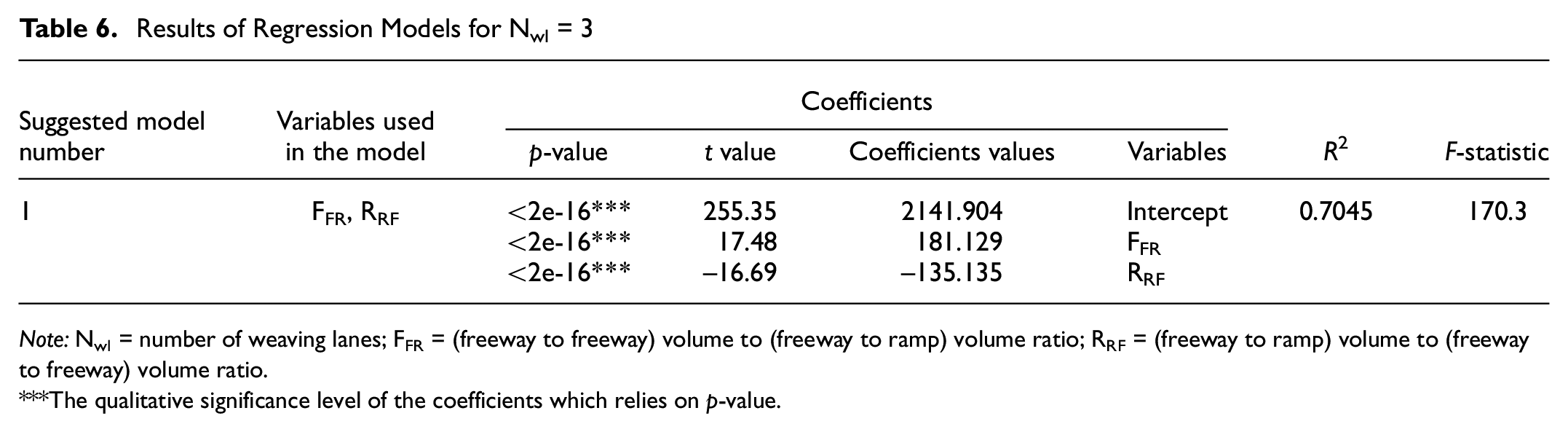
The second case relates to Nwl = 3. In this case, for regression models, data from a total of 143 simulated scenarios were used. The acceptable regression model is shown in Table 6.
Results of Regression Models for Nwl = 3
Note: Nwl = number of weaving lanes; FFR = (freeway to freeway) volume to (freeway to ramp) volume ratio; RRF = (freeway to ramp) volume to (freeway to freeway) volume ratio.
The qualitative significance level of the coefficients which relies on p-value.
According to Table 6, like Nwl = 2, there is only one model in the table that contains FFR and RRF as variables. Models containing VR and also those with disallowed p-values have been omitted from the table. The chosen model has a good value of R2 and F-statistics as well. So, the equation for the maximum length of weaving in meters is as follows.

According to Equation 4, for Nwl = 3, the only variables that change the value of Lwmax are FFR and RRF. These variables are more accurate than VR and reflect the traffic conditions better. FFR describes the weaving intensity of the freeway, and RRF describes the weaving intensity of the ramps, and these two variables have no connection with each other.
As in the previous case, the Shapiro and Breusch–Pagan tests were checked for Nwl = 3. The results of the Shapiro test for Model 1 in Table 6 are shown below.

Based on the above results, the p-value is more than 0.05, that is, with 95% confidence, the data (Model 1 in Table 6) fit the normal distribution and the normality hypothesis is accepted.
The Breusch–Pagan test was also performed to check the homoscedasticity of the model. To accept the null hypothesis of homoscedasticity for the regression model, the p-value of this test should be more than 0.05. The results of this test for model 1 in Table 6 are stated below.
Based on the above results, the p-value of the test is more than 0.05, which means that Model 1 can be used and Model 1 errors are similarly scattered (homoscedasticity is accepted).
Also, using the gvlma package, the global test for this case was performed to assess linear model assumptions. The results of this test for the Nwl = 3 model (Table 6 Model 1) is shown below in Table 7.
Summary of gvlma test for Model1 (Nwl = 3)
Note: Nwl = number of weaving lanes.
According to Table 7, as in the previous case, all assumptions are acceptable and thus there is no specific violation of Model 1 for Nwl = 3. Therefore, there is no need to use the components of the global test statistic to gain insight into which assumptions have been violated ( 35 ).
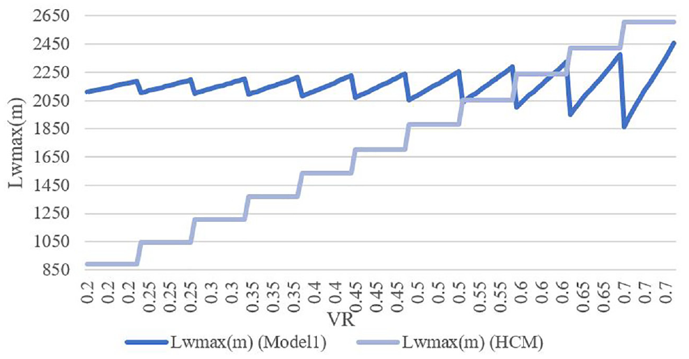
Finally, the maximum weaving length values obtained from the HCM equation and Table 6 Model 1 are compared with one another in Figure 4.
Comparison of HCM and Model 1 Lwmax values.
Based on Figure 4, like the previous case, HCM follows an upward step pattern and Model 1 has an oscillating pattern. But because of more values of VR in Nwl = 3 data, the range of change of HCM pattern is almost two times the previous case and is equal to nearly 1,716 m. Also, this range for Model 1 in Figure 4 at its maximum level is almost 594 m. It can also be seen that the variation range of Model 1 begins to increase after VR = 0.55. This is because of higher FFR and lower RRF values in scenario data after VR = 0.55. In the range of VR = 0.55–0.65, the Lwmax values of Model 1 and HCM are close to each other, so the HCM equation in this range of VR is accurate and calculates Lwmax precisely near to field values. Also, as in the previous case, it is clear that Model 1 has a far lower range of changes than HCM, and could therefore be more reliable and accurate to use and calculate the maximum weaving length value.
Conclusion
HCM 2016 has an equation to calculate the maximum length of the weaving segment. In this equation, there are only two variables of VR and Nwl. If these two variables are constant, the maximum weaving length will also be constant. If a weaving segment with constant VR and Nwl but with different traffic volumes for four weaving segment maneuvers is assumed and simulated in Aimsun, the maximum weaving segment length for different traffic scenarios will be different. It should be noted that the flow in the weaving segment is equal to the maximum weaving length capacity, and there are different capacity amounts for different values of maximum weaving length. Therefore, it can be realized that more effective variables are required in this equation to provide more accurate Lwmax values.
In HCM, traffic and geometric variables (VR and Nwl) are used to calculate the Lwmax value, which is the performance boundary between weaving and merging and diverging segments. In this study, after examining field data and conducting tests and sensitivity analyses, it was found that there were some other traffic variables besides VR that could affect the Lwmax value. Three new traffic variables (FR, FFR, and RRF) describing traffic conditions in a weaving situation have been introduced which include all macro weaving properties in a weaving segment and have been shown to be statistically meaningful. By combining field and simulation data and considering new traffic variables, new Lwmax equations for Nwl = 2 and Nwl = 3 have been produced. New traffic variables: FR, FFR, and RRF not only define the weaving situation but also display the weaving intensity. It was found that the VR variable is not sensitive to traffic intensity. These three new variables have therefore been introduced in this study. The FFR variable describes the weaving intensity of traffic on the freeway or highway. RRF describes the weaving intensity of the ramps and FR describes the intensity of both the freeway and the ramps. As a result, the VR, which is made of weaving intensity, has been divided into three more accurate variables. By doing more research, it has been found that these three new variables reflect the weaving intensity better than VR.
Footnotes
Author Contributions
The authors confirm contribution to the paper as follows: study conception and design: Behrooz Shirgir, data collection: Ali Kashani, analysis and interpretation of results: Behrooz Shirgir, Ali Kashani, draft manuscript preparation: Ali Kashani. All authors reviewed the results and approved the final version of the manuscript.
Declaration of Conflicting Interests
The author(s) declared no potential conflicts of interest with respect to the research, authorship, and/or publication of this article.
Funding
The author(s) received no financial support for the research, authorship, and/or publication of this article.