Urban Impacts of Mobile Fuel Delivery Service

Abstract

Mobile fuel delivery (MFD) uses a fueling truck to fill up personal and commercial fleet vehicles while they are parked overnight. This study used a sample data set provided by a San Francisco Bay Area company to explore the potential impacts on vehicle miles traveled (VMT), carbon dioxide (CO₂) emissions, and traffic congestion. An analysis of vehicle travel associated with gas station trips was conducted to establish a basis for comparison. Future scenarios comparing the potential impacts of scaled-up MFD services in 2030 were also developed. The study concluded that MFD services compared favorably to gas stations in relation to environmental and traffic benefits in the longer term, even though personal fueling trips tended to generate low VMT. Benefits stemmed from efficiencies achieved by fueling multiple vehicles per delivery trip, replacing car share vehicle fueling trips, and removing trips from the network during peak hours. This analysis estimated that total annual CO₂ emissions associated with fuel delivery operations in the Bay Area were 76 metric tons, which is less than a typical gas station with 97 metric tons. Under assumptions of declining demand for gasoline and significantly fewer gas stations, and with highly efficient optimized operations, mobile delivery could gain up to 5% market share for gas and not add additional VMT over the business as usual scenario.

With the rise of e-commerce, we have seen the introduction of home-delivery services for many retail goods—groceries, clothing, shoes, and so forth—and now we might add vehicle fuels to the list. The appeal of mobile fuel delivery (MFD) services to subscribers is clear—they are convenient and save time, and they replace the menial task of refueling a vehicle at a station. In this sense they also resemble home services such as housekeeping or landscaping. However, the impacts of MFD services on the wider urban community are less clear. Will MFD help or hinder urban policy goals to reduce vehicle emissions and traffic congestion? Will it increase or decrease vehicle miles traveled (VMT) or the uptake of alternative fuel vehicles?

This study addresses these questions using a sample data set provided by a MFD company in the San Francisco Bay Area. The study explores the potential impacts of MFD on urban policy goals, including:

Reducing CO₂ emissions

In an era of climate change, many levels of government around the world have set carbon dioxide (CO₂) emissions reduction goals. For example, under California’s Sustainable Communities and Climate Protection Act (SB 375), cities and regions are obligated to reduce VMT to meet CO₂ reduction targets ( 1 ). If fuel delivery services increase net VMT, they undermine these goals, whereas if they reduce VMT, they support them.

Reducing traffic congestion

Every urban metropolitan region has traffic congestion—roads clogged with traffic volumes in excess of capacity, meaning slower travel speeds. Traffic congestion can increase in two dimensions: either more hours per day or over a wider geographic extent. Significant public resources are invested annually in strategies such as commuter bus and rail services and highway and interchange capacity increases. MFD will affect these public investments by adding or reducing traffic volumes at peak hours.

Encouraging car sharing

Many cities promote car sharing as part of a more sustainable transportation system. For example, San Francisco Municipal Transportation Agency’s strategic plan includes a goal “to make transit, bicycling, taxi, ride sharing and car sharing the preferred means of travel” ( 2 ). Its car sharing policy allows for on-street and municipal garage parking spots to be designated for car share vehicles only. Fuel delivery replaces staff fueling trips, supporting the availability and affordability of these vehicles, with fewer miles traveled.

Increasing uptake of electric and alternative fuel vehicles

Increasingly, cities and states are adopting policies and building infrastructure to support electric and alternative fuel vehicles. California is a leader in this regard, with its Zero Emission Vehicle mandate, Clean Vehicle Rebate Program, and investments in electric and hydrogen fuel cell infrastructure ( 3 ). If fuel delivery services offer alternative fuels, they could lower barriers to adoption. Conversely, if they only make it easier and more convenient to own a gasoline vehicle, that could slow progress.

This study explores the potential impacts of MFD services through a review of relevant scientific literature and three analyses:

A comparison of vehicle fueling trips to grocery shopping trips;

Analysis of operations data from MFD compared with a typical gas station; and

Future scenarios comparing the potential impacts of a “business as usual” (BAU) and a “mobile fuel delivery” scenario.

Literature Review

As modern MFD services are a relatively new phenomenon, this may be the first study assessing their environmental, traffic, and other impacts as discussed in the introduction. Critical to the task was having a baseline for comparison, i.e. an understanding of gas station impacts, in order to assess whether the introduction of mobile delivery would improve or worsen impacts compared with BAU. This was a challenge, as a review of the literature found no studies directly estimating VMT associated with vehicle trips to gas stations. Instead, “adjacent” literatures that shed light on vehicle fuel purchasing behavior are discussed in this review: studies on optimal fuel station siting, driver refueling behavior, and online shopping with delivery service.

Optimal Fuel Station Location

Mobile delivery service for vehicle fuels is not an entirely new idea. In the early days of automobiles, when fueling infrastructure did not exist, there were mobile refueling services in the form of dispensing tank wagons, mobile stations, and wheeled handcarts ( 4 ). These were essentially fuel tanks mounted on wagons that circulated between home-delivery customers and corner pumps in high-demand urban locations (see Figure 1).

Figure 1.

A horse-drawn tank wagon refueling a curb pump ( 4 ).

Although presumably convenient, mobile services disappeared with the proliferation of dedicated brick-and-mortar refueling stations in the 1920s. However, they played an important role in addressing the “chicken and egg” problem facing gasoline at that time—and faced by any alternative fuel today. Vehicles utilizing alternative fuels such as electricity, hydrogen, or natural gas are impractical and unattractive to consumers while fueling stations remain few and far between, yet fuel providers will not invest in infrastructure until there is sufficient demand ( 4 – 6 ). Fueling station infrastructure in urban areas can also be inhibited by local environmental regulations, a lack of safe distribution networks, and the rising cost of real estate ( 5 ). Early MFD services helped gasoline vehicles overcome these barriers.

Driver Refueling Behavior

In the modern context of gasoline fueling infrastructure, driver surveys have been used to study vehicle refueling behavior and station location preferences. A study by Kitamura and Sperling surveyed 1,521 drivers at eight fuel stations in a range of locations in Sacramento, CA (rural town, suburbs, the central business district, and at freeway ramps) ( 7 ). They found that most trips involving fueling originated at home or work, and were linked with other activities like shopping or commuting; only 7% of drivers made home-based “unlinked” trips with the sole purpose of refueling, most commonly in suburban locations ( 7 ). Using travel time to estimate how far drivers had traveled, they found that 72% of refueling locations were within 5 min of either the trip origin or destination. About half the drivers selected a fuel station based on location: convenient to home (21%), work or school (8%), freeway (6%), and shopping (2%), or closest to where they were running out of gas (13%) ( 8 ).

Other studies have reinforced these findings. Kelley and Kuby in Los Angeles, CA followed Sperling and Kitamura’s methodology to survey 267 drivers of gasoline vehicles and 259 drivers of compressed natural gas (CNG) vehicles. They found that drivers of gasoline vehicles chose either the gas station closest to home or with the least deviation from frequently traveled routes ( 6 ). The authors noted that fueling stations belong to a class of “flow based demand” consumer goods for which people tend to stop along their way to make a purchase rather than making a special trip. Kuby et al. further found that early adopters of CNG vehicles were willing to deviate up to 6 min from their shortest path to refuel, whereas gasoline drivers were not ( 9 ). A study of gasoline station locations in Sacramento compared station distance from highways to gasoline sales and found that 51% of gallons sold were within 1 km (0.62 mi) of a highway, leading the author to conclude that they served two types of demand: home-based trips by drivers accessing the highway, and highway travelers unwilling to deviate very far to refuel ( 5 ).

The Institute of Transportation Engineers (ITE) has applied these insights about driver refueling behavior to forecast traffic impacts of new gas stations ( 10 , 11 ). They define three types of refueling trips to gas stations. A primary trip is made for the specific purpose of visiting the gas station, and mileage is considered “new” VMT. For example, a trip from home to a gas station then back home is a primary trip. A pass-by trip is made as an intermediate stop on the way to the primary trip destination, without a route diversion. For example, stopping at a gas station along the usual route driven from home to work is a pass-by trip. Pass-by trips are not new on the road network, as they would have been made even without the gas station stop, so they create no new VMT. A diverted trip requires a diversion from a usual route to specifically visit a gas station, and only the diversion mileage is considered new VMT. For example, exiting the highway to refuel is a diverted trip.

These studies demonstrate that gas station trips are highly efficient with respect to VMT. Because drivers rarely make single-purpose (primary) trips to purchase fuel, but habitually refuel as a pass-by stop on routine trips, they generate very little “extra” VMT.

Online Shopping with Delivery Service

Online shopping now accounts for 9.5% of total retail sales in the United States and is expected to keep growing strongly ( 12 ). Several empirical studies comparing CO₂ emissions from online shopping to brick-and-mortar shopping for nonfood retail goods such as clothing, books, and electronics found that home delivery can reduce CO₂ emissions under optimal conditions ( 13 – 15 ). These studies point out that the “last mile” customer trip from retail store to home is often the most energy-intensive in the supply chain, and it is expected that delivery services serving multiple customers would be more efficient than individual round-trips. Key factors that reduce potential CO₂ savings from online delivery include short travel distances from home to store, use of public transit, browsing trips, product returns, and failed delivery attempts (i.e., customer not home, no building access) ( 15 ).

Others argue that online shopping contributes to rising freight VMT and is not a full substitution for brick-and-mortar shopping but a complement resulting in more VMT overall ( 16 ). Lower prices and a greater selection of goods online induce purchases and deliveries that would not have otherwise been made. In the longer term, as physical retail stores get outcompeted by online shopping, a percentage can be expected to close, resulting in longer distance trips ( 17 ). The net outcome of these competing effects is complex and depends in large part on the type of retail good: how frequently it is purchased, average distance to stores, rates of browsing and returns. The scenario analysis in this study considered how these effects might net out in the long run for gas stations.

Methodology

This study took a three-pronged approach to estimating potential impacts of MFD services: an estimate using a proxy good, a comparative analysis of delivery and station operations data, and a future scenario analysis.

As no previous literature on MFD was found, the first method identified an analogous retail good that has been well studied: groceries. Vehicle fueling trips were compared with grocery shopping trips using travel behavior survey data. Estimates of trip frequency, trip distance, and percent primary trips for vehicle fueling trips were taken from the National Household Travel Survey (NHTS) ( 18 ), the California Household Travel Survey (CHTS) ( 19 ), the ITE Trip Generation Handbook ( 11 ), the study by Kitamura and Sperling ( 7 ), and GasBuddy customer surveys ( 20 ). Estimates of trip frequency, trip distance, and percent primary trips for grocery trips were taken from the National Household Travel Survey (NHTS) ( 19 ), US Department of Agriculture studies ( 21 ), and customer surveys by the Food Marketing Institute ( 22 ).

The second method analyzed a sample data set from a MFD company to compare the impacts of day-to-day fuel delivery operations with gas station trips. Key operations metrics were calculated for each, including average VMT per delivery/customer trip. Environmental and traffic impacts were then estimated using three parameters: 1) the percentage of primary, pass-by, and diverted trips, 2) the average mileage of each type of trip, and 3) the percentage of trips during peak hours. Data analysis was supplemented by expert interviews for a “reasonableness” check. The study area was defined as the five counties in the Bay Area with sufficient urban population density to support a MFD service: Alameda, Contra Costa, San Francisco, San Mateo, and Santa Clara counties.

The sample MFD data set was drawn during the first quarter of 2018. MFD is a 24-h, 7 days a week operation. The data included outputs from the onboard fleet telematics units of all the delivery trucks, as well as customer billing records, for a full picture of delivery truck routes and stops, the number of customer fills per stop, and the type of customer (consumer or business). Statistical software (Stata 15) and geographic information system (Esri ArcGIS) software were used to analyze the data and create charts and maps.

As operational data for gas stations was not available, travel and consumer survey data were used to calculate comparable operations metrics. Data on how often people visit gas stations, when, and how much extra driving is required to access them was obtained from the 2009 NHTS ( 18 ), the 2010 to 2012 CHTS ( 19 ), and customer surveys by the National Association of Convenience Stores (NACS) ( 23 ) and GasBuddy ( 20 ). Data from the California Annual Retail Fuel survey was used to estimate the number of fills (vehicle refueling events) per day at a typical station ( 24 ).

Finally, the resulting operational profiles were used to develop scenarios for 2030 comparing environmental and traffic impacts from a BAU scenario and a MFD scenario where these services are operating at scale and have captured noticeable market share.

Findings

Analysis 1: Comparison of Vehicle Fueling Trips with Grocery Shopping Trips

Groceries are a retail good with similar characteristics to vehicle fuels, for which the effects of e-commerce have been well studied. Studies comparing the environmental impacts of online grocery shopping with traditional brick-and-mortar shopping found potential for significant CO₂ reductions from mobile delivery. A study of a small town in England used a GIS-based model to compare VMT from home-based grocery shopping trips with a mobile delivery service and concluded that VMT could be reduced by up to 70%, with complete substitution ( 25 ). A similar study in Finland that used traffic simulation to compare e-shopping delivery service for groceries with traditional shopping estimated that VMT-related CO₂ emissions could be reduced by 88% when home deliveries allowed for unattended drop-off ( 26 ).

Groceries and vehicle fuels have similar demand characteristics and constraints for online shopping and home delivery. They are both fast-moving, consumable retail goods that have low (or nonexistent) browsing and return rates, and may be delivered without interaction with the recipient, eliminating sources of “extra” delivery VMT generated by product returns and failed deliveries ( 13 ). For example, grocery delivery services use ice-packs to protect perishable goods, whereas fuel delivery services alert vehicle owners to leave their vehicle in an accessible place with the fuel port door unlocked. They can both be ordered by “subscription” for predictable quantities at a predictable frequency, which allows for efficient delivery route optimization. Vehicle fuel is a commodity, offering higher potential efficiencies for route optimization and from eliminating trips for browsing, returns, and failed delivery attempts.

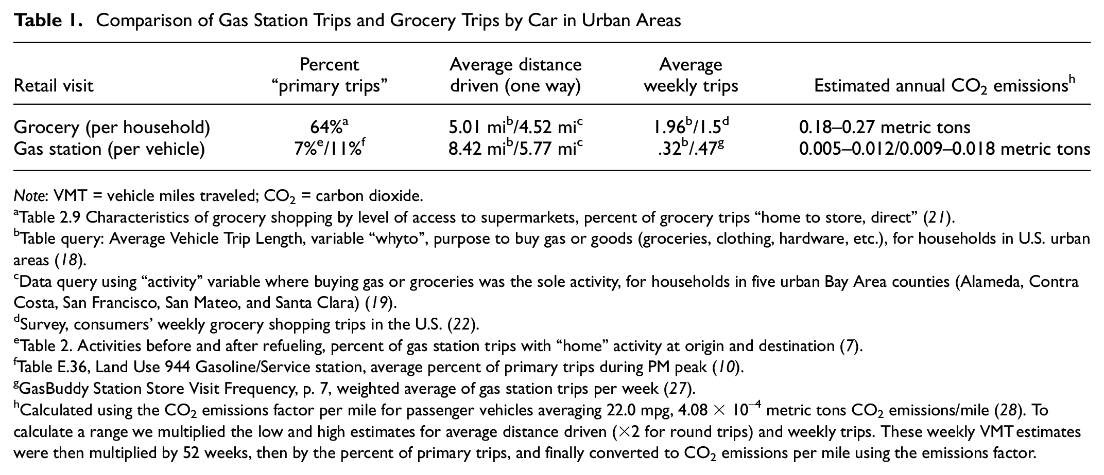
The majority of CO₂ savings from online delivery derive from the elimination of customer round-trips (primary trips), and this is where the comparison between fuels and groceries diverges. Driver refueling behavior differs from shopping trips for other retail goods, in that gas station trips are most often pass-by trips, which do not generate VMT ( 7 , 9 ). Travel survey data was used to estimate the percent of primary trips, distance driven, and number of weekly trips for groceries and gas, as shown in Table 1. Estimates differed among surveys, so a range is given in the table. All estimates are for trips by car in urban areas only.

Table 1.

Comparison of Gas Station Trips and Grocery Trips by Car in Urban Areas

Retail visit	Percent “primary trips”	Average distance driven (one way)	Average weekly trips	Estimated annual CO₂ emissions^h
Grocery (per household)	64%^a	5.01 mi^b/4.52 mi^c	1.96^b/1.5^d	0.18–0.27 metric tons
Gas station (per vehicle)	7%^e/11%^f	8.42 mi^b/5.77 mi^c	.32^b/.47^g	0.005–0.012/0.009–0.018 metric tons

Note: VMT = vehicle miles traveled; CO₂ = carbon dioxide.

Table 2.9 Characteristics of grocery shopping by level of access to supermarkets, percent of grocery trips “home to store, direct” ( 21 ).

Table query: Average Vehicle Trip Length, variable “whyto”, purpose to buy gas or goods (groceries, clothing, hardware, etc.), for households in U.S. urban areas ( 18 ).

Data query using “activity” variable where buying gas or groceries was the sole activity, for households in five urban Bay Area counties (Alameda, Contra Costa, San Francisco, San Mateo, and Santa Clara) ( 19 ).

Survey, consumers’ weekly grocery shopping trips in the U.S. ( 22 ).

Table 2. Activities before and after refueling, percent of gas station trips with “home” activity at origin and destination ( 7 ).

Table E.36, Land Use 944 Gasoline/Service station, average percent of primary trips during PM peak ( 10 ).

GasBuddy Station Store Visit Frequency, p. 7, weighted average of gas station trips per week ( 27 ).

Calculated using the CO₂ emissions factor per mile for passenger vehicles averaging 22.0 mpg, 4.08 × 10⁻⁴ metric tons CO₂ emissions/mile ( 28 ). To calculate a range we multiplied the low and high estimates for average distance driven (×2 for round trips) and weekly trips. These weekly VMT estimates were then multiplied by 52 weeks, then by the percent of primary trips, and finally converted to CO₂ emissions per mile using the emissions factor.

The main difference between grocery and gas station trips is the rate of single-purpose (primary) trips to purchase groceries or fuel. The majority of grocery trips (64%) were home-based primary trips, whereas only 7% to 11% of fueling trips were ( 7 , 11 , 21 ). As the majority of VMT was associated with primary trips, this means that gas station trips were much more efficient than grocery trips. The average trip distance was roughly similar: 4.5 to 5.0 mi for grocery trips and 5.8 to 8.4 mi for fueling trips ( 18 , 19 ). The longer trip length for fueling trips is likely to be the result of the higher rate of linked trips, that is, the majority (89% to 93%) of survey respondents were refueling as part of a longer trip to a work or to a shopping destination ( 7 , 11 ). The trip frequency was also roughly similar: 1.5 to 1.96 trips per week for grocery trips and 0.32 to 1 trip per week for gas station trips ( 7 , 18 , 22 , 27 ).

Table 1 shows a summary of these trip characteristics, including an estimated amount of annual CO₂ emissions that we calculated for grocery trips per household and gas station trips per vehicle. When added up over the course of a year, gas station trips were more efficient by an order of magnitude. Grocery delivery appears to reduce CO₂ emissions, and MFD is likely to as well, but to much a lesser extent.

Analysis 2: Comparison of Fuel Delivery Operations to Typical Gas Station

Fuel Delivery Operations Profile

Figure 2 shows the service area of the sample MFD data set, including customer stops, fuel depots, and overnight parking areas. It spans roughly 45 mi from north to south, 6 to 10 mi across, roughly 300 mi². Residential customers are predominantly male (60%), in the 35 to 50 age range. They tend to have higher levels of education (master’s and PhD) and household income (over $100,000). The majority access fuel delivery service via smartphone.

Figure 2.

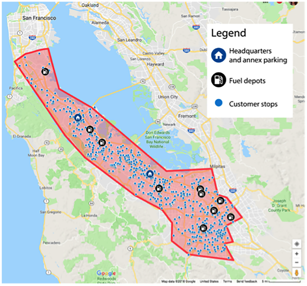
Sample fuel delivery service area.

Fuel delivery trucks start their runs from headquarters or an annex parking area, refilling at fuel depots/gas stations during delivery runs. They are heavy duty pickup trucks equipped with specially fabricated 100-gal tanks in the rear, safety certified by the California Department of Transportation, and operated by commercially licensed technicians who are hazmat (hazardous materials) trained. The trucks also carry spill containment kits, fire extinguishers, and meters certified by the state Weights and Measures Board. The trucks make prescribed tours that are generated daily by route optimization software.

In the sample data set we analyzed, the trucks drove 2,919 mi total, an average of 504 mi per weekday. About 13% of the total weekly mileage was on the weekend. Altogether the trucks made 843 stops, with 727 (86%) for customer deliveries, as illustrated in Figure 3. The remaining 118 stops were at fuel depots to replenish their fuel tanks or to parking areas at the end of their runs. The average VMT per stop was 3.5 mi (2,919 mi/843 stops). Each truck traveled an average of 36 mi and made nine customer stops on a typical run, or tour, as defined by a loop starting and ending at a parking lot or fuel depot. There was a wide variation in the number of customer stops on a given run, ranging from 1 stop with 50 fills for a fleet customer, to 22 stops in a residential area dense with household customers.

Figure 3.

Total vehicle miles traveled by MFD trucks.

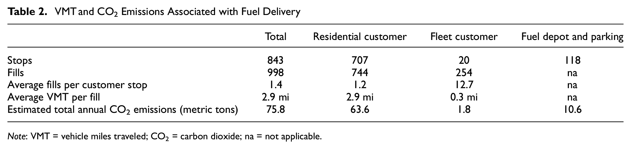
In the sample data set, 998 fills were completed: 744 vehicles belonging to private individuals and 254 vehicles belonging to commercial fleet customers, including trucks and car share vehicles. About 25% of vehicles filled belonged to commercial customers. Operations delivering fuel to these fleet vehicles were highly efficient. In the sample, 20 delivery stops were made for fleet customers, with an average of 12.7 fills per stop. For residential customers, improved efficiency was achieved via a “multiple vehicle discount” for vehicles within a certain radius, incentivizing neighbors to recruit each other. According to billing data in which this discount was applied, residential customers averaged 1.2 fills per delivery stop.

One of the most important metrics for comparing the environmental impacts of MFD with gas station trips is VMT per fill. The average VMT per fill for delivery was 2.9 mi (2,919 mi/998 fills). When disaggregated by customer type, fleet customers had a much lower VMT per fill compared with residential customers. As fleet customers had an average of 12.7 fills per stop, the average VMT per fill was only 0.3 mi (3.5 mi per stop/12.7 fills per stop). For home-delivery customers with an average of 1.2 fills per stop, the average was 2.9 mi traveled per fill (3.5 mi per stop/1.2 fills per stop).

CO₂ emissions associated with fuel delivery were calculated as a function of VMT, using the CO₂ emissions factor for the type of pickup trucks in use (18.0 mpg, for 4.994 × 10⁻⁴ metric tons CO₂ emissions/mile) ( 28 ). As shown in Table 2, total annual CO₂ emissions are estimated at 75.8 metric tons per year, the majority generated by residential deliveries.

Table 2.

VMT and CO₂ Emissions Associated with Fuel Delivery

	Total	Residential customer	Fleet customer	Fuel depot and parking
Stops	843	707	20	118
Fills	998	744	254	na
Average fills per customer stop	1.4	1.2	12.7	na
Average VMT per fill	2.9 mi	2.9 mi	0.3 mi	na
Estimated total annual CO₂ emissions (metric tons)	75.8	63.6	1.8	10.6

Note: VMT = vehicle miles traveled; CO₂ = carbon dioxide; na = not applicable.

When considering traffic congestion impacts, the two most important metrics are when and where trips are being added to the network, as trips made on low-volume roads and during off-peak hours are unlikely to add to congestion. In the Bay Area, and many other regions, peak hours are from 6:00 to 10:00 a.m. and 3:00 to 7:00 p.m. on weekdays. MFD data showed that just 9% of their trip departures were during peak hours for traffic congestion. As illustrated in Figure 4, their operational pattern is almost perfectly inverse to the classic peak traffic hours. Given this pattern, only 1 in 10 fuel delivery trips is potentially contributing to traffic congestion. As the majority of miles traveled are on uncongested parts of the road network, in residential neighborhoods, we concluded they have a negligible effect on traffic congestion.

Figure 4.

Histogram of MFD departure times and peak traffic hours.

Gas Station Operations Profile

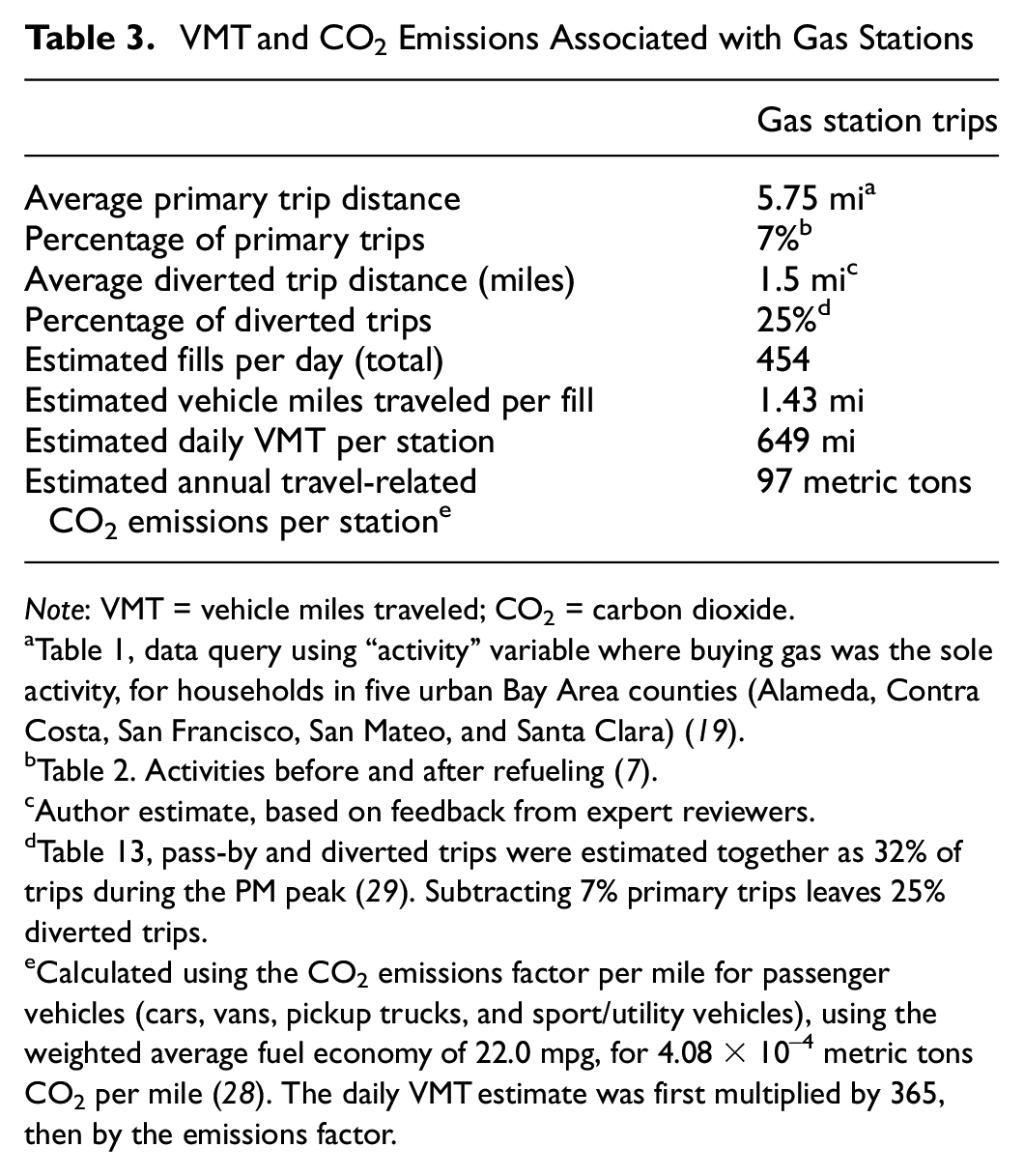
There are currently about 400 gas stations in the MFD study area, as estimated from Census data. To compare the environmental and traffic impacts of these gas stations with MFD required an understanding of how often people visit, when, and how much extra driving is required to access them. Lacking direct operational data, developing a profile of typical gas station operations was a challenge. The first approach relied on ITE methodology and traffic surveys published in the Trip Generation Manual and Handbook (10, 11). However, the resulting VMT estimates were considered too high by expert reviewers. A new methodology based on travel survey data was developed, with results summarized in Table 3.

Table 3.

VMT and CO₂ Emissions Associated with Gas Stations

	Gas station trips
Average primary trip distance	5.75 mi^a
Percentage of primary trips	7%^b
Average diverted trip distance (miles)	1.5 mi^c
Percentage of diverted trips	25%^d
Estimated fills per day (total)	454
Estimated vehicle miles traveled per fill	1.43 mi
Estimated daily VMT per station	649 mi
Estimated annual travel-related CO₂ emissions per station^e	97 metric tons

Note: VMT = vehicle miles traveled; CO₂ = carbon dioxide.

Table 1, data query using “activity” variable where buying gas was the sole activity, for households in five urban Bay Area counties (Alameda, Contra Costa, San Francisco, San Mateo, and Santa Clara) ( 19 ).

Table 2. Activities before and after refueling ( 7 ).

Author estimate, based on feedback from expert reviewers.

Table 13, pass-by and diverted trips were estimated together as 32% of trips during the PM peak ( 29 ). Subtracting 7% primary trips leaves 25% diverted trips.

Calculated using the CO₂ emissions factor per mile for passenger vehicles (cars, vans, pickup trucks, and sport/utility vehicles), using the weighted average fuel economy of 22.0 mpg, for 4.08 × 10⁻⁴ metric tons CO₂ per mile ( 28 ). The daily VMT estimate was first multiplied by 365, then by the emissions factor.

The CHTS was used to find the average trip distance for gas station trips in the study area using the “activity” variable ( 19 ). For each trip reported by drivers, they also reported up to three activities that took place during the trip, for example, “work/job duties” or “eat meal at a restaurant.” The activity variable “service private vehicle (gas, oil, lube, repair)” was filtered to include trips for which only one activity was reported. Trips with a duration of longer than 10 min were also filtered out, as refueling trips typically take 2 to 3 min and 75% of customers remained at the station for less than 10 min ( 27 ). The resulting average trip distance for primary trips to the gas station was 5.77 mi, meaning a total of 11.5 VMT (round-trip from home and back). The estimate from Kitamura and Sperling was used for the percentage of primary trips (7%) ( 7 ).

No studies or surveys reporting trip distances for diverted trips to gas stations were found, so an estimate was of 1.5 mi was selected in discussion with experts. This means an average diverted trip contributed 3 mi round-trip. For pass-by trips, the estimate from Cunningham et al. was used to calculate the percent of diverted trips ( 29 ). They estimated pass-by and diverted trips together as 32% of trips during the PM peak; subtracting 7% for primary trips leaves 25% diverted trips.

To estimate the number of fills per day at a typical gas station, data from the California Annual Retail Fuel survey were used. In 2016, 2.189 billion gal of fuel were sold in the study area, or nearly 6 million gal per day, by 1,321 gas stations ( 24 ). This means each station sold about 4,540 gal per day (6 million gal/1,321 trips). This estimate passed a “reasonableness” test when compared with the California Energy Commission’s average fuel dispensed per day estimate of 4,400 gal ( 30 ). Assuming that the average fill-up was 10 gal, that means 454 vehicles refueled at each station, per day. Then 32 primary trips (454 trips × 7%) and 113 diverted trips (454 trips × 25%) give a total of 145 trips with VMT each day. VMT was calculated by multiplying the number of trips by trip distance, for 369 mi associated with primary trips (32 trips × 5.8 mi × 2 trips), and 340 mi associated with diverted trips (113 trips × 1.5 mi × 2), which sums to 649 mi per station per day. Finally, 1.4 mi per fill (627 mi/454 fills) and 97 metric tons of CO₂ per year (649 mi × .000408 CO₂/mile × 365 days) were calculated.

As for when drivers purchase fuel, the ITE estimates that about half (48%) of gas station trips are made during peak congestion hours, 6:00 to 10:00 a.m. and 3:00 to 7:00 p.m., according to their surveys ( 11 ). A recent customer survey by NACS also found that most respondents (58%) made refueling trips during peak traffic congestion hours ( 23 ). Results from a question survey asking “what time of day do you often purchase gas?” are shown in Figure 5. Another consumer survey by GasBuddy showed that afternoon hours (noon to 3:00 p.m.) are also a popular time for purchasing fuel, presumably over a lunch break ( 27 ).

Figure 5.

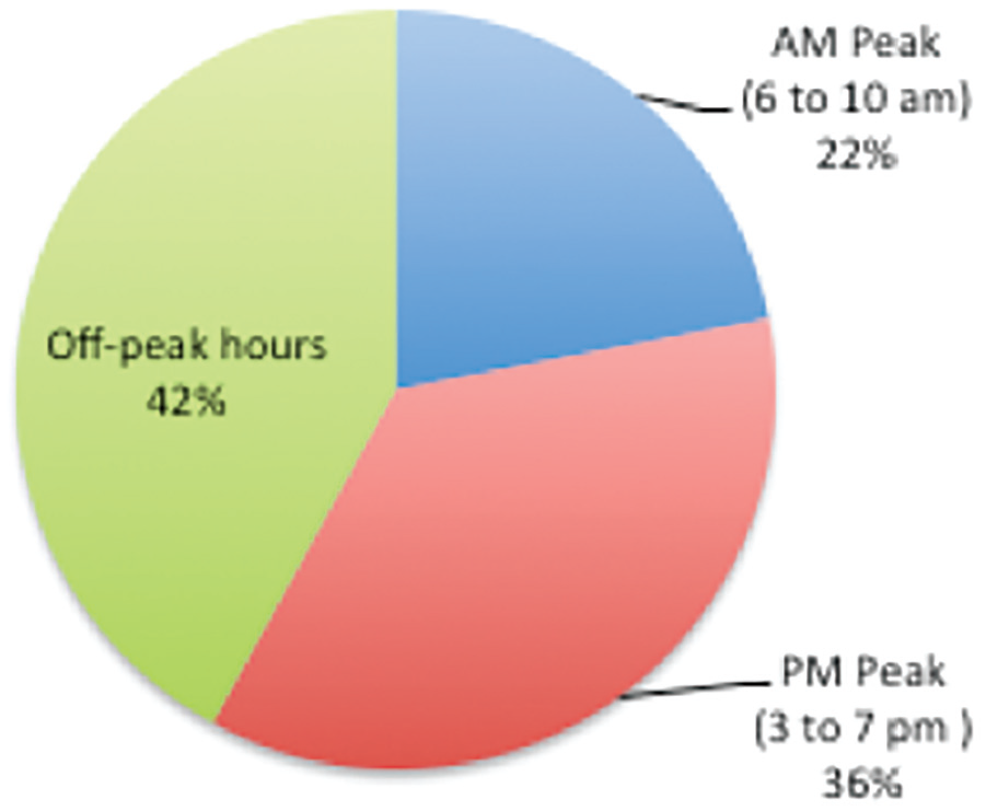
Customers’ preferred time of day for fuel purchase ( 23 ).

These findings show that most gas station trips traditionally take place during peak commute hours, meaning they are contributing to traffic congestion. Even pass-by trips, which do not generate extra VMT, can be a source of travel delay as they involve queuing and turning movements. For each gas station trip that is removed from the network peak hours, we would expect a very small time saving that would only make a noticeable impact at scale.

Comparison of Fuel Delivery Operations with Gas Station Operations

Table 4 summarizes key metrics from the analyses of empirical data for fuel delivery and gas stations, taken from Tables 2 and 3.

Table 4.

Comparison of Key Metrics for Mobile Delivery and Gas Station Travel

Metric	Mobile delivery	Gas station
Fills per stop	1.2: residential customer 12.7: fleet customer	1
Vehicle miles traveled per fill	2.9 mi: residential customer 0.3 mi: fleet customer	1.4 mi
Most likely time of day delivery/trip made	Off peak	PM peak

Individual gas station trips averaged 1.4 mi per fill, meaning that mobile delivery must have a lower VMT per fill to achieve VMT reductions. In the fuel delivery data set analyzed, VMT averaged 2.9 mi per fill for residential customers and 0.3 mi per fill for fleet customers. Therefore VMT impacts were mixed: higher for residential customers but lower for fleet customers. VMT per fill for home delivery will decrease as the density of residential customers increases. The overall average VMT per fill for all customers depends on the ratio of residential customers to fleets: more fleet customers means greater VMT reductions.

Analysis 3: Future Scenarios for 2030

To consider how environmental and traffic impacts might add up over time, future scenarios for the year 2030 compared a BAU scenario extrapolating current trends into the future with a MFD scenario in which delivery services are widely available. The year was chosen to be at least 10 years in the future, as a decade was considered the amount of time necessary for fuel delivery services to scale up and gain enough market share to have a noticeable impact on fuel stations, and to start seeing land use changes. In both future scenarios the percentage of primary, diverted, and pass-by trips is expected to remain the same, as driver preferences to avoid route diversions have proven stable over time.

Gas Station Closure Trend

As this study is deeply concerned with the distances that drivers must travel to refuel, there is an emerging trend in the retail fuel industry that merits mention: the disappearance of gas stations in central business districts, which are not being replaced, leading to “gas deserts” ( 31 ). An annual count of gas stations shows ∼1% fewer each year, as illustrated in Figure 6 ( 32 ). From 1994 to 2013, the number of retail gas stations in the United States fell from 202,800 to 152,995—a 25% decline ( 33 ). This trend is related in part to gas stations becoming increasingly larger on average, both in relation to the number of pumps and floor area, often with a convenience store or fast food restaurant in the building ( 29 ). At the same time, gasoline sales have been in decline overall as fuel efficiency standards rise and alternative fuels gain market share ( 34 ). As a result, gas stations are consolidating and becoming fewer and farther between.

Figure 6.

Declining number of gas stations in the United States ( 32 ).

Gas stations are disappearing in dense urban areas where high value land parcels are being converted from car-oriented land uses to people-oriented uses like residential, office, and retail. As land values rise, even parcels that require, for instance, expensive remediation for leaky gas storage tanks have become feasible for redevelopment. For example, there were over 60 gas stations in Manhattan in 2004, but just 32 in 2017 ( 35 , 36 ). Former gas station sites have been converted into housing, shopping centers, and office buildings ( 37 ).

Business as Usual Scenario

The BAU scenario assumed that gas stations will have continued to disappear from city centers, up to 2030. Evidence the gas desert trend in San Francisco was found in Oil Price Information Service data ( 38 ). Figure 7 shows the locations of gas stations that closed and opened during the period 2007 to 2018. Although there were closures and openings throughout the Bay Area, the pattern seen on the map is particular to downtown San Francisco, San Jose, and Oakland. About four times as many stations have closed as opened, and closures are concentrated in the densest downtown cores, where they have not been replaced.

Figure 7.

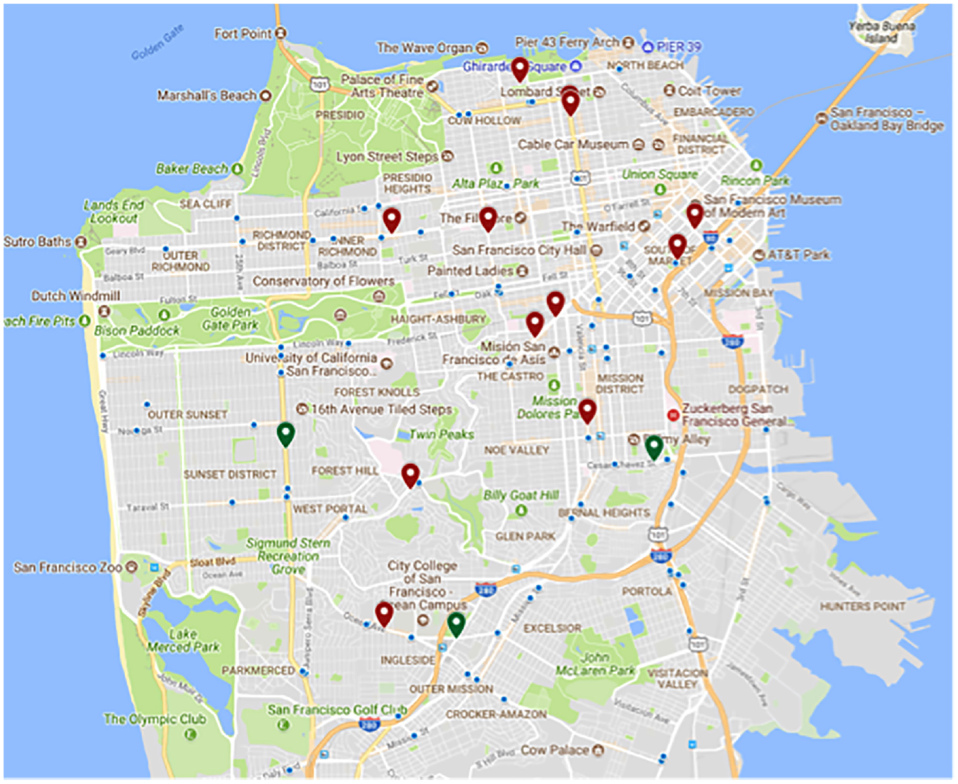
Gas station closures (red) and openings (green) in San Francisco, 2007–2018 ( 38 ).

Time series data from Census County Business Patterns data was used to forecast how many gas stations might be left in 2030 ( 39 ). Figure 8 shows gas stations in the study area from 2005 to 2016—a decline of 31% since 2005 ( 39 ). The highest rates of closure were in urbanized counties: −28% San Francisco, −22% San Mateo, and −16% Santa Clara. This is a strong 10-year trend that may continue indefinitely as fuel consumption decreases owing to increasing fuel economy, uptake of alternative fuel vehicles, and reduced personal car-ownership as car sharing and transport network companies grow market share.

Figure 8.

Number of gas stations in urban Bay Area counties ( 39 ).

Figure 9 shows an extrapolation of the gas station closure trend to the year 2030. A simple linear regression predicts the number of fuel stations in the study area will fall from 1,000 today to roughly 750 in a decade. The decline since 2006 is nearly linear, giving the trendline a high goodness-of-fit (R²) statistic of 0.8. This forecast predicts that 25% of the gas stations in the study area today will be gone by 2030 if the current trend continues. A more conservative estimate of 15% was used for this analysis. One reason that gas stations are disappearing is declining fuel sales. The US Energy Information forecast for gasoline sales in the near term is nearly flat, with 0.3% growth projected for 2018 and 2019 ( 40 ). In the longer term, demand for gasoline is projected to decline such that 2030 consumption will be 34% lower than 2018 ( 41 ). Again, a more conservative estimate of 10% lower fuel demand in 2030 was used for this analysis. Fewer stations means that drivers will need to travel longer distances to access stations, on average. To account for this, one scenario assumed that primary and diverted trips will increase by 0.1 mi.

Figure 9.

Number of gas stations in urban Bay Area counties—2030 Forecast ( 39 ).

The amount by which trip distance increases will depend on which stations close, and how many drivers are forced to take longer routes accordingly. In central business districts where station closures are most likely, fewer residents own fewer cars, so extra driving to access gas stations is not expected to have a significant impact. In the rest of the urban area, where land prices are not rising as steeply, station closures are most likely where there is more competition, declining demand, or both, and are likely to affect more drivers.

Mobile Fuel Delivery Scenario

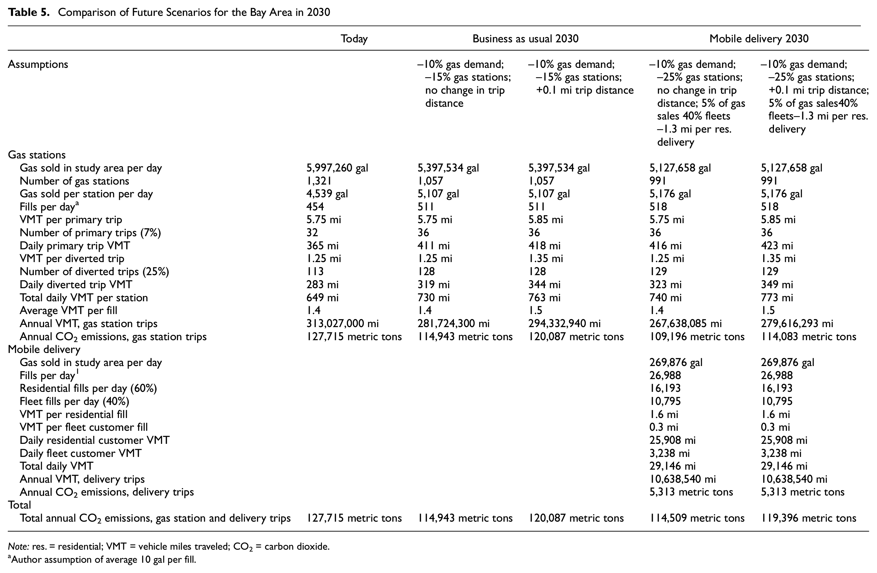
The MFD scenario built on the BAU scenario, but assumed that MFD is available throughout the urban area and operating at scale, accounting for 5% of fuel sales in 2030. Increased competition will contribute to the trend of disappearing gas stations, so 5% fewer stations are assumed, compared with the BAU scenario. Since BAU assumed 15% fewer stations, that means 20% fewer stations in the MFD scenario. The results displayed in Table 5 represent an optimized future operation that has achieved efficiencies of scale. VMT per residential fill is assumed to have decreased from 2.9 mi today to 1.6 mi. The proportion of fleet customers is assumed to have grown from 25% to 40%. These scenarios assumed the same delivery trucks are in use, so CO₂ emissions for delivery operations were calculated using the CO₂ emissions factor for light duty trucks.

Table 5.

Comparison of Future Scenarios for the Bay Area in 2030

	Today	Business as usual 2030		Mobile delivery 2030
Assumptions		–10% gas demand; –15% gas stations; no change in trip distance	–10% gas demand; –15% gas stations; +0.1 mi trip distance	–10% gas demand; –25% gas stations; no change in trip distance; 5% of gas sales 40% fleets–1.3 mi per res. delivery	–10% gas demand; –25% gas stations; +0.1 mi trip distance; 5% of gas sales40% fleets–1.3 mi per res. delivery
Gas stations
Gas sold in study area per day	5,997,260 gal	5,397,534 gal	5,397,534 gal	5,127,658 gal	5,127,658 gal
Number of gas stations	1,321	1,057	1,057	991	991
Gas sold per station per day	4,539 gal	5,107 gal	5,107 gal	5,176 gal	5,176 gal
Fills per day^a	454	511	511	518	518
VMT per primary trip	5.75 mi	5.75 mi	5.85 mi	5.75 mi	5.85 mi
Number of primary trips (7%)	32	36	36	36	36
Daily primary trip VMT	365 mi	411 mi	418 mi	416 mi	423 mi
VMT per diverted trip	1.25 mi	1.25 mi	1.35 mi	1.25 mi	1.35 mi
Number of diverted trips (25%)	113	128	128	129	129
Daily diverted trip VMT	283 mi	319 mi	344 mi	323 mi	349 mi
Total daily VMT per station	649 mi	730 mi	763 mi	740 mi	773 mi
Average VMT per fill	1.4	1.4	1.5	1.4	1.5
Annual VMT, gas station trips	313,027,000 mi	281,724,300 mi	294,332,940 mi	267,638,085 mi	279,616,293 mi
Annual CO₂ emissions, gas station trips	127,715 metric tons	114,943 metric tons	120,087 metric tons	109,196 metric tons	114,083 metric tons
Mobile delivery
Gas sold in study area per day				269,876 gal	269,876 gal
Fills per day¹				26,988	26,988
Residential fills per day (60%)				16,193	16,193
Fleet fills per day (40%)				10,795	10,795
VMT per residential fill				1.6 mi	1.6 mi
VMT per fleet customer fill				0.3 mi	0.3 mi
Daily residential customer VMT				25,908 mi	25,908 mi
Daily fleet customer VMT				3,238 mi	3,238 mi
Total daily VMT				29,146 mi	29,146 mi
Annual VMT, delivery trips				10,638,540 mi	10,638,540 mi
Annual CO₂ emissions, delivery trips				5,313 metric tons	5,313 metric tons
Total
Total annual CO₂ emissions, gas station and delivery trips	127,715 metric tons	114,943 metric tons	120,087 metric tons	114,509 metric tons	119,396 metric tons

Note: res. = residential; VMT = vehicle miles traveled; CO₂ = carbon dioxide.

Author assumption of average 10 gal per fill.

As shown in Table 5, under these assumptions, the CO₂ emissions from mobile delivery operations are projected to be 5,313 metric tons annually in 2030. However, this will be offset by declining CO₂ emissions from gas station trips owing to the background trend of declining gas sales. In the first BAU scenario, all factors were held constant except for a 10% decline in gas sales and 15% fewer gas stations. CO₂ emissions declined from 127,715 to 114,944 metric tons annually, a reduction of 12,772 metric tons because of lower gas sales. The second BAU scenario assumed that average gas station trip distance would increase by 0.1 mi, owing to fewer gas stations. As a result, projected CO₂ emissions increased to 120,944 metric tons annually, meaning that 5,144 tons can be attributed to driving longer distances.

In the first mobile delivery scenario, 2030 CO₂ emissions from gas station trips are projected to be lower: 109,196 metric tons, owing to lower gas station sales. Adding CO₂ emissions from mobile delivery brings projected 2030 CO₂ emissions to a total of 114,509 metric tons. Note that this is roughly equivalent to the BAU scenario. This means that if the operational efficiencies tested are achieved, mobile delivery could account for 5% of gas sales without adding extra CO₂ emissions, all things being equal.

The second mobile delivery scenario assumed that average gas station trip distance increased by 0.1 mi resulting from fewer gas stations. As a result, 2030 CO₂ emissions are projected to be higher, 114,083 metric tons, and when CO₂ emissions from mobile delivery are added, the total amounts to 119,396 metric tons. In this case, CO₂ emissions are slightly lower than the BAU scenario. This indicates that if average gas station trip distance increases as the number of gas stations decreases, mobile delivery could help reduce CO₂ emissions on net. The more average trip distance increases, the more efficient delivery is, by comparison. These findings indicate that at scale, if the operational efficiencies tested are achieved, mobile delivery could offset rising CO₂ emissions resulting from fewer gas stations located further apart.

Summary of Findings and Conclusions

Vehicle Miles Traveled

A fundamental question of this study was whether MFD would increase or decrease VMT compared with gas stations. The first of the three analyses showed VMT reduction is more likely. This analysis, a comparison of fuel delivery with grocery delivery, showed similar impacts for direction of change (lower VMT), but not magnitude (lower impact). VMT was reduced owing to the elimination of primary trips (i.e., individual trips to and from the store). Trips to grocery stores and gas stations were of similar distance and frequency, but only a small portion (7% to 11%) of gas station trips were primary trips so the impact of removing them was smaller than for grocery stores. Fuel delivery vehicles travel a prescribed route that is more efficient than individual gas station trips.

The second analysis, a comparison of fuel delivery with gas station trips, showed that VMT reduction depended on two key factors: residential customer density and the percentage of fleet customers. Individual gas station trips averaged 1.4 mi per fill, meaning that mobile delivery must have a lower VMT per fill to achieve VMT reductions. In the fuel delivery data set analyzed, VMT averaged 2.9 mi per fill for residential customers and 0.3 mi per fill for fleet customers. Therefore VMT impacts were mixed: higher for residential customers but lower for fleet customers. The overall average VMT per fill for all customers depends on the ratio of residential to fleets: more fleet customers means greater VMT reductions. To achieve similar VMT impacts as gas stations, MFD’s VMT per fill needs to decline from 2.9 mi to about 1.4 mi. This could be achieved by increasing customer density and by reducing the operational miles required for trips to fuel depots and off-duty parking.

The third analysis, a comparison of future scenarios for 2030, showed that VMT projections are sensitive to assumptions about demand for gas, the number of gas stations, and average trip distance to access a gas station. Mobile delivery could fill a gap as gas stations disappear. Under assumptions of declining demand for gasoline and fewer gas stations, if the operational efficiencies tested are achieved, mobile delivery could gain up to 5% market share for gas and not add additional VMT over the BAU scenario. If a declining number of gas stations results in longer gas station trips, mobile delivery could help offset the increased VMT from extra driving.

CO₂ Emissions

This study considered CO₂ emissions impacts as a direct function of VMT. This method was an oversimplification, as CO₂ emissions are also related to engine type, vehicle speed, and acceleration profile, but was sufficient to determine the direction and magnitude of the impacts that may be expected. CO₂ emissions for gas trips were estimated using an emissions factor for passenger vehicles, whereas CO₂ emissions for fuel delivery used an emissions factor for light duty trucks.

The first analysis concluded that gas station and grocery trips are similar, and so impacts of delivery services would be similar. Delivery is expected to reduce CO₂ emissions for grocery trips by replacing individual round-trips with more efficient prescribed delivery tours. CO₂ emissions for gas station trips were found to be an order of magnitude lower that grocery trips owing to the high percentage of pass-by trips for gas. Per household, annual CO₂ emissions for grocery trips were estimated as 0.18 to 0.27 metric tons, and 0.005 to 0.018 metric tons for gas station trips. Therefore CO₂ emissions impacts for gas delivery are expected to have the same direction of change (lower VMT), but lower magnitude.

The second analysis estimated annual CO₂ emissions associated with today’s MFD operations in the Bay Area as 76 metric tons, less than a typical gas station with 97 metric tons. CO₂ emissions impacts at scale will depend on the operational efficiencies achieved by increasing the density of residential customers and increasing the percentage of fleet customers, as previously discussed.

Traffic Congestion

MFD operations are helping to relieve traffic congestion by eliminating peak-hour gas station trips made by individual drivers. Gas station trips contribute to peak-hour traffic congestion: driver surveys show that the majority refuel during peak hours. Even though most gas station trips are pass-by trips, there is a small time cost to the queuing and turning movements required to access gas stations during peak hours, which will have impacts at scale. The analysis of the sample fuel delivery data set in the second analysis revealed that only 9% of trip departures were during peak traffic congestion hours, minimizing traffic impacts. If operations remain off-peak focused, this could help reduce traffic volumes at peak hours.

Other Impacts

The sample data set analyzed in this study found that fuel delivery had the greatest VMT and CO₂ emissions reduction impacts on fleets. This impact depends on how many fleet vehicles are parked together at the same location and how far they would otherwise have to be driven to refuel. As shown in Table 2, fleet customers averaged 12.7 fills per delivery stop, compared with 1.2 for residential customers. That means that each fuel delivery eliminated 26 trips to and from gas stations (13 round trips) from the road network. This amounted to a net VMT saving of 1.1 mi per fleet vehicle, per fill (1.43 mi per gas station fill minus 0.3 mi per fleet customer fill). The total annual impacts of fleet fuel delivery were calculated as 14,900 mi (254 fills/week × 1.13 mi/fill × 52 weeks) reduced VMT and 6.1 metric tons reduced CO₂ emissions.

As noted in the introduction, car sharing vehicles are a type of fleet that could benefit from fuel delivery. If fuel delivery replaces car share customer responsibility for refueling, that makes it more attractive and supports low car-ownership lifestyles. In some car sharing models, vehicles are dispersed throughout a service area and staff must first drive to where they are parked. In this case, two car trips are eliminated by fuel delivery—the trip to the car share vehicle and the gas station trip.

Finally, the third analysis noted a long-term trend underway of urban gas stations disappearing. In our future scenario with MFD, we projected increased competition over time and at scale, advancing the disappearance of gas stations. Fewer gas stations means increased trip distances and perhaps higher prices in the long run. If the operational efficiencies tested in the scenario are achieved, mobile delivery could offset and even reduce rising CO₂ emissions resulting from extra driving. Those unable to afford mobile delivery or lacking Internet access or a bank account may face higher prices. Such barriers to delivery service could be removed by offering alternate scheduling and payment methods.

Footnotes

Acknowledgements

The author thanks Daniel Chatman of UC Berkeley, Jeff Lidicker of California Air Resources Board, and Dan Tischler and Drew Cooper of San Francisco County Transportation Agency, whose expertise and feedback helped to guide this analysis, as well as Pierson Stoecklein and Scott Hempy from Filld, for providing the the sample dataset and insights into MFD operations.

Author Contributions

The author confirms sole responsibility for the following: study conception and design, data collection, analysis and interpretation of results, and manuscript preparation.

Declaration of Conflicting Interests

The author(s) declared no potential conflicts of interest with respect to the research, authorship, and/or publication of this article. The author was hired as an external consultant by a third party to author this study.

Funding

The author(s) disclosed receipt of the following financial support for the research, authorship, and/or publication of this article: This study was funded by Filld, a MFD company based in Mountain View, CA.

References

CARB. Proposed Update to the SB 375 Greenhouse Gas Emission Reduction Targets. Updated Final Staff Report. California Air Resources Board, Sacramento, CA, 2018. https://www.arb.ca.gov/cc/sb375/sb375_target_update_final_staff_report_feb2018.pdf.

SFMTA. On-Street Car Sharing Pilot Program. Evaluation Report. San Francisco Municipal Transportation Agency, 2017. https://www.sfmta.com/sites/default/files/projects/2017/Carshare_eval_final.pdf.

CARB. Zero Emission Vehicle Program. California Air Resources Board, Sacramento, CA, 2018. https://www.arb.ca.gov/msprog/zevprog/zevprog.htm.

Melaina

M. W.

Turn of the Century Refueling: A Review of Innovations in Early Gasoline Refueling Methods and Analogies for Hydrogen. Energy Policy, Vol. 35, No. 10, 2007, pp. 4919–4934.

Nicholas

M. A.

Driving Demand: What Can Gasoline Refueling Patterns Tell Us about Planning an Alternative Fuel Network?

Journal of Transport Geography, Vol. 18, No. 6, 2010, pp. 738–749.

Kelley

Kuby

On the Way or around the Corner? Observed Refueling Choices of Alternative-Fuel Drivers in Southern California. Journal of Transport Geography, Vol. 33, 2013, pp. 258–267.

Kitamura

Sperling

Refueling Behavior of Automobile Drivers. Transportation Research Part A: General, Vol. 21, No. 3, 1987, pp. 235–245.

Sperling

Kitamura

Refueling and New Fuels: An Exploratory Analysis. Transportation Research Part A: General, Vol. 20, No. 1, 1986, pp. 15–23.

Kuby

M. J.

Kelley

S. B.

Schoenemann

Spatial Refueling Patterns of Alternative-Fuel and Gasoline Vehicle Drivers in Los Angeles. Transportation Research Part D: Transport and Environment, Vol. 25, 2013, pp. 84–92.

10.

ITE. ITE Trip Generation Manual, 10^th ed., Volume 1. Institute of Transportation Engineers (ITE), Washington, D.C., 2017.

11.

Hooper

K. G.

Trip Generation Handbook, 3rd ed., Publications Errata, Institute of Transportation Engineers (ITE), Washington, D.C., 2018.

12.

Census. Quartely Retail E-Commerce Sales, 1st Quarter 2018. US Census Bureau, Economic Indicators Division, Washington, D.C., 2018. https://www.census.gov/retail/mrts/www/data/pdf/ec_current.pdf.

13.

Edwards

J. B.

McKinnon

A. C.

Cullinane

S. L.

Comparative Analysis of the Carbon Footprints of Conventional and Online Retailing: A “Last Mile” Perspective. In International Journal of Physical Distribution & Logistics Management ( Halldórsson

Á.

, ed.), Vol. 40, No. 1/2, 2010, pp. 103–123.

14.

Carling

Han

Håkansson

Meng

Rudholm

Measuring Transport Related CO₂ Emissions Induced by Online and Brick-and-Mortar Retailing. Transportation Research Part D: Transport and Environment, Vol. 40, 2015, pp. 28–42.

15.

Wiese

Toporowski

Zielke

Transport-Related CO₂ Effects of Online and Brick-and-Mortar Shopping: A Comparison and Sensitivity Analysis of Clothing Retailing. Transportation Research Part D: Transport and Environment, Vol. 17, No. 6, 2012, pp. 473–477.

16.

Visser

Nemoto

Browne

Home Delivery and the Impacts on Urban Freight Transport: A Review. Procedia - Social and Behavioral Sciences, Vol. 125, 2014, pp. 15–27.

17.

Visser

E.-J.

Lanzendorf

Mobility and Accessibility Effects of B2C E-Commerce: A Literature Review. Tijdschrift voor economische en sociale geografie, Vol. 95, No. 2, 2004, pp. 189–205.

18.

NHTS. National Household Travel Survey. Federal Highway Administration, Washington, D.C., 2009. https://nhts.ornl.gov/.

19.

Caltrans. 2010-2012 California Household Travel Survey. California Department of Transportation, Sacramento, CA, 2013. https://www.nrel.gov/transportation/secure-transportation-data/tsdc-california-travel-survey.html.

20.

GasBuddy, and Cuebiq. Foot Traffic Report and Driving Trends for the Fuel and Convenience Store Industry: 2017 Year in Review and 2018 Forecast. GasBuddy, Boston, MA, 2018. https://business.gasbuddy.com/wp-content/uploads/2018/01/FootTrafficReportQ42017.pdf.

21.

USDA. Access to Affordable and Nutritious Food: Measuring and Understanding Food Deserts and their Consequences. US Department of Agriculture, Economic Research Service, Washington, D.C., 2009. https://www.ers.usda.gov/webdocs/publications/42711/12716_ap036_1_.pdf.

22.

FMI. US Grocery Shopping Trends. Food Marketing Institute, Arlington, VA, 2017. https://www.statista.com/statistics/251728/weekly-number-of-us-grocery-shopping-trips-per-household/.

23.

NACS. How Consumers Behave at the Pump. Fuels Resource Center, 2017. http://www.convenience.org/YourBusiness/FuelsCenter/Pages/How-Consumers-Behave-at-the-Pump.aspx#.WulHEdMvyV4. Accessed May 2, 2018.

24.

CEC. 2016 California Annual Retail Fuel Outlet Report Results (CEC-A15). California Energy Commission, Energy Assessment Division, Sacramento, CA, 2017. http://www.energy.ca.gov/almanac/transportation_data/gasoline/piira_retail_survey.html.

25.

Cairns

Delivering Supermarket Shopping: More or Less Traffic?

Transport Reviews, Vol. 25, No. 1, 2005, pp. 51–84.

26.

Siikavirta

Punakivi

Karkkainen

Linnanen

Effects of E-Commerce on Greenhouse Gas Emissions: A Case Study of Grocery Home Delivery in Finland. Journal of Industrial Ecology, Vol. 6, No. 2, 2002, pp. 83–97.

27.

GasBuddy, and Cuebiq. Foot Traffic Report for the Fuel and Convenience Store Industry, Q1 2017. GasBuddy, Boston, MA, 2017. https://www.iab.com/wp-content/uploads/2017/08/2017.07_FootTrafficReportQ2_CuebiqGasBuddy.pdf.

28.

EPA. Greenhouse Gases Equivalencies Calculator - Calculations and References. Environmental Protection Agency, Washington, D.C., 2018. https://www.epa.gov/energy/greenhouse-gases-equivalencies-calculator-calculations-and-references.

29.

Cunningham

C. M.

Findley

D. J.

Schroeder

Foyle

R. S.

Traffic Operational Impacts of Contemporary Multi-Pump Island Fueling Centers. ITE Journal-Institute of Transportation Engineers, Vol. 81, No. 6, 2011, p. 24.

30.

CEC. Summary of California Vehicle and Transportation Energy. California Energy Commission, Sacramento, CA, 2018. www.energy.ca.gov/almanac/transportation_data/summary.html.

31.

CSP. Fueling Feast or Famine. CSP Magazine, Vol. 27, No. 11, 2016, pp. 40–48.

32.

NPN. Market Facts Annual Station Count. National Petroleum News, 2013. https://www.afdc.energy.gov/uploads/data/data_source/10333/10333_gasoline_stations_year.xlsx.

33.

Gross

America’s Gas Stations Are Running out of Time. Slate, 2016. http://www.slate.com/articles/business/the_juice/2016/06/why_america_s_gas_stations_are_running_out_of_time.html. Accessed May 10, 2018.

34.

UMTRI. Gasoline Use at Lowest Rate in Three Decades. University of Michigan Transportation Research Institute, 2015. http://www.umtri.umich.edu/what-were-doing/news/gasoline-use-lowest-rate-three-decades. Accessed May 2, 2018.

35.

Nir

S. M.

With Gas Station’s Closing, a Fuel Desert Expands in Manhattan. The New York Times, 2016. https://www.nytimes.com/2016/04/16/nyregion/a-gas-station-closes-in-soho-making-lower-manhattan-a-gasoline-desert.html. Accessed May 20, 2018.

36.

Quirk

M. B.

There Are Only 32 Retail Gas Stations Left in Manhattan. Consumerist, 2017. https://consumerist.com/2017/07/19/there-are-only-32-retail-gas-stations-left-in-manhattan/.

37.

Reeves

Mapping the Many Gas Stations Lost to NYC’s Development Boom. Curbed, New York, NY, 2017. https://ny.curbed.com/maps/gas-station-map-housing-nyc. Accessed May 20, 2018.

38.

OPIS. Custom Gas Station Data Report. Oil Price Information Service, 2018. https://www.opisnet.com/.

39.

Census. County Business Patterns Datasets. US Census Bureau, 2017. https://www.census.gov/programs-surveys/cbp/data/datasets.html.

40.

EIA. Short-Term Energy Outlook. US Energy Information Administration, Washington, D.C., 2018. https://www.eia.gov/outlooks/steo/.

41.

EIA. Annual Energy Outlook 2018. US Energy Information Administration, Energy Consumption by Sector and Source, Washington, D.C., 2018. https://www.eia.gov/outlooks/aeo/.