




Abstract
Short-term prediction of traffic flow is essential for the deployment of intelligent transportation systems. In this paper we present an efficient method for short-term traffic flow prediction using a Support Vector Machine (SVM) in comparison with baseline methods, including the historical average, the Current Time Based, and the Double Exponential Smoothing predictors. To demonstrate the efficiency and accuracy of the SVM method, we used one-month time-series traffic flow data on a segment of the Pan Island Expressway in Singapore for training and testing the model. The results show that the SVM method significantly outperforms the baseline methods for most prediction intervals, and under various traffic conditions, for the rolling horizon of 30 min. In investigating the effect of the input-data dimension on prediction accuracy, we found that the rolling horizon has a clear effect on the SVM’s prediction accuracy: for the rolling horizon of 30–60 min, the longer the rolling horizon, the more accurate the SVM prediction is. To look for a solution for improvement of the SVM’s training performance, we investigate the application of k-Nearest Neighbor method for SVM training using both actual data and simulated incident data. The results show that the k- Nearest Neighbor method facilitates a substantial reduction of SVM training size to accelerate the training without compromising predictive performance.
Short-term prediction of traffic flow is crucial for Advanced Travelers Information Systems (ATIS) and Advanced Traffic Management Systems (ATMS). Reliable traffic flow forecasting is important for developing real-time traffic control systems. For these reasons, timely and accurate traffic flow prediction has been a subject of intensive research for a long time. Traffic flow prediction approaches so far can be broadly classified into the time-series analysis approach and the machine learning approach ( 1 ). Techniques associated with the time-series analysis approach cover a wide range, from historical average ( 2 ) to Kalman Filtering ( 3 – 6 ), Exponential Smoothing ( 7 , 8 ), and Autoregressive Moving Average (ARIMA) models ( 7 , 9 – 11 ). Techniques associated with the machine learning approach include k-Nearest Neighbor ( 12 – 15 ), Artificial Neural Network ( 16 – 18 ), and Support Vector Machine (SVM) ( 19 – 21 ).
Although a considerable number of traffic flow prediction methods have been deployed, each of them has certain advantages and limitations. The time-series analysis approach is simple and easy to understand, but the models following this approach typically only capture linear relationships. Consequently their performance deteriorates under non-linear conditions ( 22 , 23 ). For example, the ARIMA model cannot capture traffic dynamics given its underlying assumption that the time-series data are stationary with unchanged average ( 22 , 24 ). The ARIMA’s extension, the seasonal ARIMA, model can address dynamics of traffic conditions, but the outlier detection and parameter estimation of the seasonal ARIMA models are time-consuming ( 25 ).
The second category, the Machine Learning approach, is able to deal with complex non-linear data and is thus widely used in traffic flow forecasting. The Artificial Neural Network (ANN) method ( 26 – 28 ) is naturally a methodological candidate for forecasting with multiple inputs and outputs. The ANN model, with its parallel structure and learning capability, is suitable for solving complex problems like prediction of traffic parameters ( 29 ). However, the method can be prone to poor generalization and performance on previous unseen data during the test phase ( 30 ). In addition, the ANN model requires a large amount of data for training, so its prediction accuracy is subject to the sample size.
Support Vector Machines (SVM), introduced by ( 31 ), is a family of machine learning algorithms. SVM possesses a good generalization capability and computational efficiency, and is very robust in high dimensions. SVM can effectively address the shortcomings of ANN by using not only the minimal risk strategy to train, but also the structure risk minimization strategy to minimize the upper bound of the error ( 30 ). Through the application of the Kernel function, SVM can map a non-linear problem in the low dimensional input space to a linear problem in the high-dimensional feature space ( 23 ). Because of its ability to outperform most other learning algorithms, it has been successfully applied to many applications such as biology ( 32 ) and financial time-series analysis ( 33 ). In traffic engineering, SVM has been widely used in many domains, such as traffic incident detection ( 34 ), traffic safety ( 35 , 36 ), and travel time prediction ( 29 , 37 , 38 ).
In the area of traffic flow prediction SVM has received a large body of research work: ( 39 ) proposed an accurate multi-steps traffic flow prediction model based on SVM in which the input vectors were comprised of actual traffic volume and different types of input vectors, including combinations of the space-time data and the historical pattern data. The test results showed that the proposed SVM model had a mean relative error of 12.8%; ( 40 ) introduced a hybrid PSO-SVR forecasting method which uses particle swarm optimization (PSO) to search optimal support vector regression (SVR) parameters to get a higher precision with less learning time. The results of extensive comparison experiments indicated that the proposed model can get better forecasting accuracy than other comparative algorithms, including the conventional SVM, ARIMA, and Back Propagation Neural Network (BPNN); ( 41 ) proposed a hybrid optimization algorithm which combines PSO with a genetic algorithm to search the optimal parameters of a least square support vector machine (LSSVM). The experimental results showed that the hybrid-LSSVM model yields better prediction ability and relatively high computational efficiency compared with non-heuristic and heuristic algorithms; and ( 42 ) proposed a traffic flow prediction model based on LSSVM which automatically determines the LSSVM model with two parameters in the appropriate value by Fruit Fly Optimization Algorithm (FOA). The experiment results showed that the LSSVM combined with FOA (LSSVM-FOA) has obvious advantages in traffic flow forecasting accuracy: the LSSVM-FOA model achieves the global optimum quickly and provides better accuracy than the single LSSVM model, RBF neural network (RBFNN), and LSSVM combined with particle swarm optimization algorithm (LSSVM-PSO). Other literatures on the application of SVM techniques for traffic flow prediction can be seen in ( 21 , 23 , 43 ).
In reviewing the literature, we found that a majority of previous research effort had focused on deployment of optimization algorithms for parameters selection for the SVR model such as GA-LSSVM, PSO-LSSVM, and FOA-LSSVM. The works used relatively short prediction intervals and relatively small amounts of data for SVM training. Little is known of the research on critical concerns such as the effect of rolling horizon (input vector dimension) on prediction accuracy, how the SVM’s prediction performance changes in a wider range of prediction intervals, how the similarity of patterns between training and testing sets affect the SVM’s prediction accuracy, and what can be done—apart from optimal parameter selection—to improve the SVM’s prediction performance? Some of these concerns can be explored using simpler tools such as the k-Nearest Neighbor algorithm.
The k-Nearest Neighbor (k-NN) algorithm is a non-parametric technique that considers distances between members in the learning sets and the target data by Euclidean distance ( 12 , 14 , 44 ). In estimating the predicted data, the k-NN algorithm does not need all samples but only the nearest data to obtain the results more quickly, so it is suitable for applications that require short computational time such as traffic flow forecasting ( 13 ). The k-NN algorithm has been widely used for traffic flow forecasting: ( 13 ) proposed two-tier k-NN for traffic flow forecasting and found that the algorithm can meet real-time requirements for accuracy and reliability of short-term traffic flow forecasting; ( 12 ) applied k-NN method to form the training dataset for local linear wavelet neural network (LLWNN) in a kNN-LLWNN model for the online short-term prediction of traffic volumes. The results show that kNN-LLWNN performs comparably with LLWNN and SVM, while its running time is much lower than LLWNN and SVM; ( 45 ) used a hybrid prediction model (kNN-SVM) for short-term traffic flow forecasting and found that the forecasting accuracy of the kNN-SVM model is better than other traditional prediction models, including the k-NN, SVR, and neural networks specifically.
In this paper we present an investigation into application of the SVM model for short-term time-series traffic flow prediction and application of the k-NN method for improvement of SVM training. We evaluate the overall performance of SVM prediction using field data collected from a segment of the Pan Island Expressway of Singapore over a wide range of prediction intervals. We investigate the effect of rolling horizon (input vector dimension) on prediction accuracy. We explore the effects of pattern similarity on prediction performance using the k-NN method under various traffic flow conditions.
The remainder of this paper is structured as follows: the next section introduces essential theoretical background of SVM and SVR algorithms that is relevant for traffic flow forecasting. We then explain the basic notions used in this study: the SVM model and baseline predictors, and the data and performance measures. This is followed by a presentation of the prediction results by the SVM method in comparison to the baseline predictors and a discussion of the effect of rolling horizon on prediction performance. In particular, in this section we present the effect of the k-NN method on SVM training efficiency using both actual and simulated data, and address some issues for online applications. Finally, we summarize essential conclusions and findings from this research.
Support Vector Machines
SVM is one of the supervised learning algorithms in the field of machine learning. It is widely used for classification and regression problems. The basic idea of SVM is to find a hyper plane in the feature space so that all classified data are farthest from the plane ( 30 ). The SVM theory for classification problems can be extended to a non-linear regression problem (SVR) for traffic flow forecasting. In the following paragraphs, we introduce briefly the essence of the SVR theoretical background in light of those provided by ( 30 ) and ( 46 ), with reference to ( 23 ).
Given a group of traffic flow data in a training dataset of a specific location:

where
the inputs
the responses
N is the number of training data.
The prediction of the traffic flow of the i time interval is denoted as
The basic idea of SVR is to map the data input

where
the functions
b is a bias value.
The coefficients w and b are obtained by minimizing the objective function:

where C is a constant and

The




where C is a pre-specified value and
The Lagrange multipliers

where

The equality constraints may be dropped if the Kernel contains a bias term b that has been considered in the Kernel function. In this case, the regression function is reduced to:

The Kernel function
The RBF Kernel function has the form:

where
Methodology
Basic Notations
The basic notations used in this study include:
Prediction interval
Rolling horizon (
Rolling step
Time-series prediction: from the definitions of

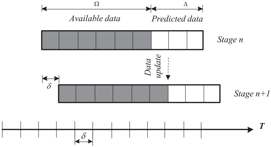
The rolling horizon approach for time-series traffic flow prediction.
Time-Series Traffic Flow Prediction: Mode of Operation
This study uses the rolling horizon approach provided by (
47
) for short-term traffic volume prediction. In the rolling horizon approach (Figure 1) the time window (T) is divided into several stages, each consisting of short intervals known as data granularity. In each stage, data in the rolling horizon
The predicted data (in stage n) can be used for traffic control or assignment applications, and then the time horizon is forwarded by the rolling step
The SVM Prediction Model
In this study, the SVR is deployed by using the Python programming language and Keras library. To avoid numerical difficulties during the calculation, the prediction starts with data scaling in both training and testing sets from large numeric ranges into smaller numeric ranges of
Parameter selection: For the use of RBF Kernel, first we determine the model parameters (C and
In this experiment, in the search space, the parameter
For SVM training, the empirical NN method (see sub-section underneath) can be used to locate the most similar traffic patterns from the historical database (HDB) within the desirable rolling horizon. We denote the volume predicted by the SVM method at time
Baseline Predictors
Historical Mean Predictor (HMP)
The historical profiling is simply the series of historical mean volumes in successive intervals. The use of the historical average rests on the method’s simplicity, and on the observation that there exist high correlation coefficients of traffic counts among weekdays in the segment (
50
). Since the test set basically includes data on weekdays, the historical average is calculated from traffic volumes only on weekdays in

In the first stage of this experiment
Current Time-Based Predictor (CTP)
The current time-based predictor predicts traffic volumes by projection of traffic volume at the current time t. Let

Since the CTP simply projects the current traffic volume to the future flow, it is likely that the CTP incurs high errors for long prediction intervals, especially under dynamic conditions.
Double Exponential Smoothing Predictor (ESP)
The exponential smoothing method weights past observations using exponentially decreasing weights: recent observations are given higher weights in forecasting than the older observations ( 51 ).



where
Note that in Equations 12–14, t indicates the index of the current interval, not the calendar time as in the other predictors. For a prediction interval,
Data
The data used for prediction involves field traffic volumes obtained on a four-lane segment (ID.80007766) with the length of 400 m, between Adam and Kheam Hock roads, along the Pan Island Expressway (Figure 2). The data are collected via traffic detectors and aggregated for the whole direction every 5 min, retrieved and stored in a HDB. Data in a day associates with 288 intervals of 5 min. From the HDB, data on traffic volume for the whole month of October 2013 was selected and screened for training and testing.
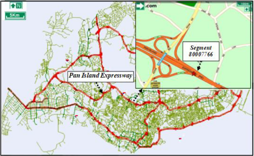
The study segment in the Singapore expressway system.
The experiment involves employing several datasets. Let



Performance Measures
Mean Absolute Percentage of Error (MAPE) is the primary statistic used as key performance measure. Let

where N is the number of observations. MAPE is calculated for each day separately, and the parameter of interest is the mean of the MAPE (or
Results
Overall Predictive Performance
The prediction with training set

Errors of the overall prediction by different methods (
Figure 3 shows that the predictive performances by all predictors (except HMP) deteriorate as
The SVM offers excellent performance for small
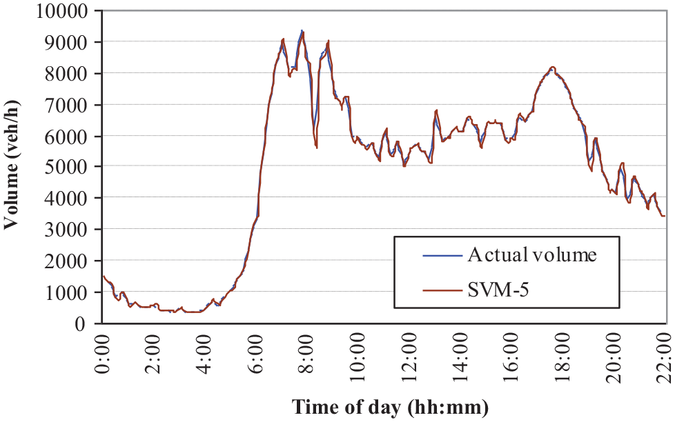
Support vector machine (
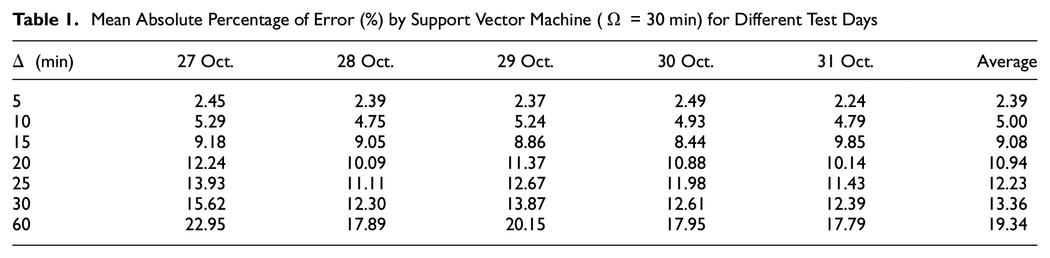
Table 1 shows the predicted errors by SVM method for individual test sets. The errors are bounded in a small range, especially for
Mean Absolute Percentage of Error (%) by Support Vector Machine (
Effect of Rolling Horizon
To explore how SVM prediction accuracies change with
Figure 5 plots the prediction errors for three values of


Effect of rolling horizon on prediction accuracy.
The magnitudes of the two errors depend on the model complexity. A simple model (small
Nearest Neighbor Method for SVM Training (NN-SVM)
SVM provided good performances in various sets of
The k-Nearest Neighbor (k-NN) algorithm is a non-parametric technique that makes use of a database to search for data that are similar to the test data. The k-NN considers distances between members in the learning sets and the test data using Euclidean distance. In this study, we consider the relative distance between each instance in the learning data with the corresponding instance in the test data. Given a learning set, the Nearest Neighbor seeks to find a day that has the most similar patterns to the test day. Let

where
Given the calculated results, the distances are sorted from small to large, so are the historical data according to the distance. Finally, k-nearest neighbors are found based on the selection criteria. In this experiment, we aim to obtain the five closest matches and the five farthest matches as follow: we use the aggregated data for the whole month of October, named as dataset

The three learning sets were trained and tested with the same test sets in

Mean absolute percentage of error (MAPE) of nearest neighbor-support vector machine with
As can be seen from Figure 6, the prediction with
We further explored the features of the NN method by addressing the question of whether the NN-SVM is workable under more dynamic and unexpected conditions like incidents and whether the similarity effect helps to enhance prediction under incidents. Ideally, these questions should be explored and verified with actual data. However, since the availability and the quality of incident data do not warrant a prediction that requires good data resolution and incident attributes, we attempted to investigate these issues under simulated incident conditions. The simulated segment has geometrical similarity to the actual site (segment 80007766) of four lanes in each direction, except for the length that is extended from 400 m to 1,000 m. Three levels of traffic demand representing the volumes during the night time, day time, and a.m. peak, derived from a typical day in the HDB are created in

where the low, medium, and high volumes are specified at 1,000, 4,000, and 7,000 vph, respectively.
And three incident scenarios:

Given the sets









for 180 min of simulation time, decomposed into:
from start to 60th min: warm-up period
from 61st min to 120th min: no incident
from 121st min to 150th min: incident
from 151st min to 180th min: no incident.
The necessary number of repetitions should be strictly estimated through an iterative process. However, because of the limited time for the high number of scenarios, we empirically determined the number of repetitions as five runs for each scenario where the random seeds are consecutively assigned as 20, 30, 40, 50, and 60. The characteristics of these five random seeds are that they have the same the traffic demand and incident scenario, but vehicles are released randomly by the simulation generator, thus traffic patterns are similar but not identical.
To examine the similarity effect of the NN-SVM method, we used data from one random seed for the test set, and data from the other four random seeds, together with the remaining eight scenarios for training. Data on traffic volumes is collected every 2 min. The parameters of prediction model are set as: rolling horizon
We apply the concept of the aforementioned distance metric to define the closeness between the test data and the training data, sorted by distances, then classified the training data into three training sets: Train-All for the whole training set, Train-NN for the smallest distances (six datasets), and Train-farNN for the farthest distances (six datasets). As can be expected, cases of four random numbers in the training are included in Train-NN with relative distances from 0.04 to 0.06. The other scenarios have higher distance values, ranging from 0.27 to 0.52. Figure 7 shows the result of the NN-SVM prediction. Again, the prediction results with Train-NN are very close to that with Train-All for all prediction intervals. By contrast, the prediction with Train-farNN incurs high errors, even with
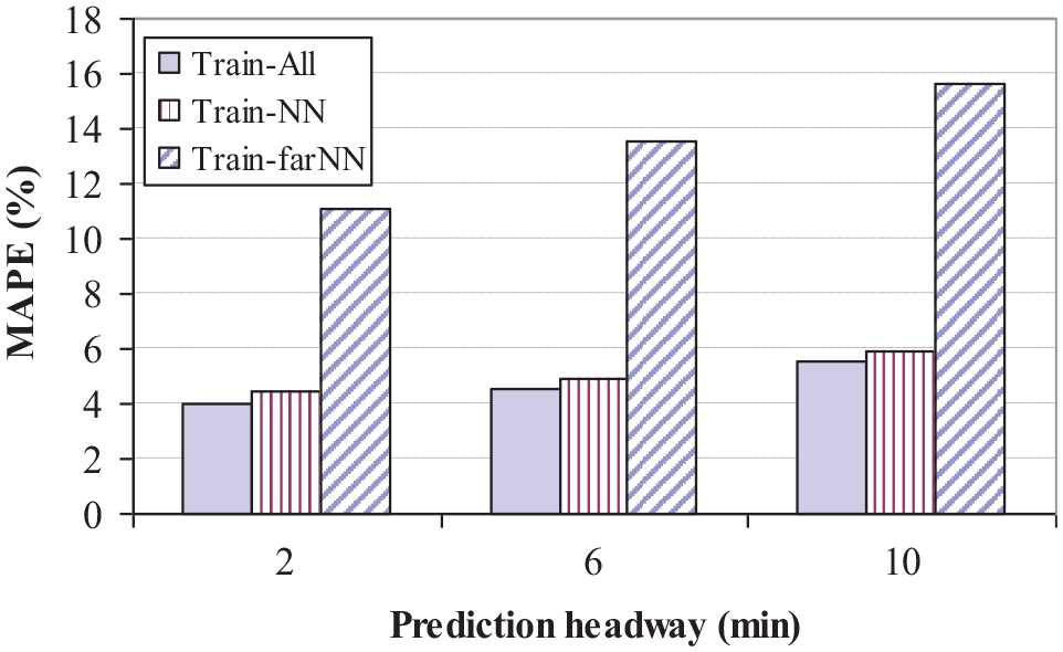
Nearest neighbor-support vector matrix with simulated incident data.
Discussion
By using actual and simulated data, we have explored the merits of applying the k-NN method to improve SVM prediction. It is appealing that the method allows training at a very high speed. For example: for the prediction
It should be noted that there is a tradeoff between distance, training time and accuracy: a high distance threshold will result in less data being cut off, the prediction accuracy enhances with a compromise in the training time. On the contrary, a low distance threshold enables fast training, but the data may become too sparse to provide enough representation power, leading to poorer performance. There is no rule universally established for distance selection, since it depends on data and application. However, a certain threshold can be determined empirically associated with a desirable accuracy and training speed.
The k-NN method presented above is for offline training, and is applied for 24 h. Offline training uses a simple forecasting approach by directly compute the average of the k-NNs, while more sophisticated approaches in the literature generate forecasting values by weighting the k-NNs according to their distances to the current state vector ( 14 ). This is particularly relevant to online-forecasting where different instances in the rolling horizon have different relevancy to the current time, represented by relative weights. Therefore, for online application the method should be modified to adapt to the real-time requirement.
Recall that
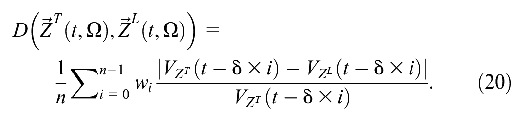
where
The k-NN distance estimation presented in Equations 17 and 20 is empirical and heuristic in nature. It follows the form of MAPE that targets the lowest prediction error. Alternative techniques of dissimilarity metric commonly used in literature include Euclidean distance, square distance ( 44 ) and absolute distance, and windowed Nearest Neighbor ( 53 ). The acronym “similarity,” being the inverse of “distance” can also be used. In essence, all of these techniques attempt to learn relevant information before the current time.
Conclusion
This paper presents an investigation into the performance of the SVM method for short-term traffic flow prediction in comparison with traditional time-series traffic flow prediction methods, including the Historical Mean predictor, the Current Time Based predictor, and the Double Exponential Smoothing. To improve SVM training, we investigate the application of the k-NN method for the training using actual data, and further reinforce the merit of the k-NN approach with extensive simulated data. From the results, the following findings are summarized:
The performance of the SVM-based predictor is significantly better than the baseline predictors for prediction intervals of less than 30 min. It has excellent performance particularly for small
The rolling horizon has a clear effect on SVM’s prediction accuracy: the longer the rolling horizon, the more accurate the prediction is, because of the capability of SVM in solving complex classification problems in a high-dimensional space.
In SVM training, the similarity of patterns between training and testing sets governs the prediction accuracy. By contrast the training size is not critical: given a reasonable training size, if the training data contain sufficient support vectors to construct hyperplanes to represent the input properly, the other data can be discarded.
The k-NN is an attractive tool for SVM training. In retrieving the most similar patterns in the learning data for SVM training, the method allows substantial reduction of training size to accelerate the training, without compromising the prediction quality.
The attractive features when combining k-NN with SVM should be deployed for online applications: a hybrid kNN-SVM model can be established, where k-NN works as a pre-processing component that looks for the most similar patterns, whose similarity is estimated by assigning relative “weights” for different intervals in the rolling horizon. This conceptual methodology shall be elaborated by a system architecture.
Furthermore, we note that the first finding stated above is the comparative results between SVM and relatively simple prediction tools. It is worth exploring the comparative performance of SVM against other advanced machine learning algorithms, such as the ANN method, and this is a subject of our future research.
Footnotes
Acknowledgements
The authors would like to gratefully acknowledge the Land Transport Authority of Singapore for its provision of data used in this study.
Author Contributions
The authors confirm contribution to the paper as follows: study conception and design: Toan and Hung; data collection: Toan; analysis and interpretation of results: Toan and Hung; draft manuscript preparation: Toan. All authors reviewed the results and approved the final version of the manuscript.
Declaration of Conflicting Interests
The author(s) declared no potential conflicts of interest with respect to the research, authorship, and/or publication of this article.
Funding
The author(s) received no financial support for the research, authorship, and/or publication of this article.
Data Accessibility Statement
Data used in this research is provided by the Land Transport Authority of Singapore on request for research purpose.