
Abstract
An analysis was performed to evaluate the impact of changing the transit signal priority (TSP) requesting threshold on bus performance and general traffic, using field-generated data exclusively. Route 217, a conventional bus route that uses a dedicated short-range communication (DSRC)-based TSP system as part of its normal day-to-day operations, was analyzed over a three-month period from May 2019 through August 2019. The requesting thresholds evaluated for Route 217 were 3, 2, and 0 min, which stipulate how far behind schedule the bus must be to request TSP. For each requesting threshold, bus performance was evaluated through on-time performance (OTP), schedule deviation, travel time, and dwell time, while the traffic analysis was performed by evaluating split failure, change in green time, and the frequency at which TSP was served. A combination of observational and statistical analyses concluded with convincing evidence that OTP, schedule deviation, and travel time improve as the requesting threshold approaches zero with negligible impacts on general traffic. As the requesting threshold changed from 3, to 2, to 0 min, OTP increased 2.0% and 2.5%, respectively; mean schedule deviation improved by 15.9 s and 20.9 s, respectively; and travel time decreased at 75% of timepoints. Meanwhile, negative impacts to traffic occurred if an increase in split failure was measured after TSP was served, a phenomenon observed a maximum of once every 43 min. Thus, it is concluded that bus performance improves as the requesting threshold approaches zero with inconsequential impacts on general traffic.
Transit Signal Priority (TSP) is an operational strategy that facilitates the movement of transit vehicles through intersections controlled by traffic signals. The purpose of TSP is to reduce travel time and the variability in travel time of transit vehicles ( 1 ). The Utah Department of Transportation (UDOT) and the Utah Transit Authority (UTA) have partnered together to implement TSP and evaluate its impacts on bus performance and general traffic.
The TSP system uses dedicated short-range communications (DSRC) technology for UTA buses to communicate with the signal controllers at the intersections along Route 217. The TSP software for this deployment was based on the Multi-modal Intelligent Traffic Signal System (MMITSS) developed for the Connected Vehicle (CV) Pooled Fund Study. It was adapted to match Utah’s needs and is referred to as MMITSS-UT ( 2 ).
After implementing TSP in November 2017, researchers determined that equipped buses were on time 3% more often than non-equipped buses ( 2 , 3 ). Optimization was then needed to further improve the effectiveness and efficiency of the operation. While a TSP system has many parameters that can be optimized, this research will optimize the operation outside of a simulation and through field data exclusively by performing a sensitivity analysis of the TSP requesting threshold parameter. The requesting threshold is the point at which TSP is requested and is defined by how far behind schedule the transit vehicle must be to request TSP.
It is expected that as the requesting threshold approaches zero and TSP is requested and consequently served more often, there will be greater positive impacts on bus performance and greater negative impacts on general traffic. Therefore, the purpose of this research is to determine the optimal requesting threshold to balance the positive impacts of TSP on bus performance with the negative impacts on general traffic. The results of this research will improve the effectiveness and efficiency of TSP on Route 217, help other agencies understand the impact of changing the requesting threshold for their TSP deployments, and help UDOT and UTA meet their goal of improving mobility through optimization and innovation.
This paper presents the findings from a literature review, a description of the TSP deployment, the analysis methodology for the research, and the results of the requesting threshold analysis. Finally, conclusions to the research are presented.
Literature Review
This section reviews TSP strategies and treatments, transit vehicle detection, the TSP communication system, evaluating TSP operations, and findings from previous TSP evaluations.
TSP Strategies and Treatments
Passive TSP strategies operate continuously, regardless of whether a transit vehicle is present, and do not require detection or a TSP request. Thus, passive priority treatments are simpler and optimize the system for transit without requiring requests from individual vehicles. Common treatments of passive strategies include fixed signal timing that favors the movement of a transit vehicle, a predetermined green extension that occurs when the transit vehicle is scheduled to pass through the intersection, or a dedicated right-of-way for transit vehicles ( 1 , 4 ).
Active priority strategies require transit vehicle detection and a means to request TSP. Active TSP strategies can be classified as either conditional or unconditional. Unconditional priority means that TSP is requested whenever the transit vehicle is detected and does not consider other criteria. Conditional priority, on the other hand, means that certain conditions need to be met before generating the request, such as the transit vehicle being late, satisfying a minimum occupancy requirement, or time since the last request was granted.
Conditional strategies thus require additional information which is usually provided from the transit vehicle’s on-board computer or the signal controller. The additional information required for conditional priority complicates TSP deployments, yet it is “most commonly accepted as an initial TSP application…assuming that buses would be issued priority only if they are behind schedule or have a certain number of persons onboard the bus” ( 5 ).
Adaptive priority strategies are the most complex and grant TSP while simultaneously trying to optimize given traffic performance criteria. Adaptive, or real-time, TSP strategies take into account both automobile and transit vehicle arrivals when considering granting TSP. Active priority treatments are then applied with the higher purpose of meeting specific measures of effectiveness (MOEs), such as minimizing person or vehicle delay. Thus, an adaptive strategy considers the trade-offs between transit and traffic vehicular delay or person delay and allows adjustments of signal timing based on prevailing conditions. The most common active priority treatments include early green (EG), green extension (GE), and transit-only signals ( 1 ).
The EG treatment, sometimes referred to as red truncation, is an active strategy that shortens the amount of green time of previous, conflicting phases to permit the phase that serves the transit vehicle to turn green earlier than normal. The benefits of EG are minimal because the transit vehicle must still wait at the red light and only profits by the number of seconds earlier that the light turns green.
GE is a strategy that lengthens the amount of green time allocated to the phase that serves the transit vehicle. Transit vehicles that benefit from GE are saved from having to wait at a red light for the green time allocated to all other conflicting movements to take place. Thus, GE, when served, offers a relatively large delay reduction, but only to the small fraction of buses that arrive at an intersection near the end of green ( 6 ).
When transit vehicles operate on the same roadway as non-transit vehicles, a transit-only signal facilitates the movement of the transit vehicle through the intersection by eliminating conflicting movements. A transit-only signal treatment is usually implemented through phase insertion, which occurs when the special transit-only phase in inserted within the normal signal sequence ( 1 ). Common examples of a transit-only signal through phase insertion include the insertion of a bus-only left-turn phase or a through movement phase to permit bus queue jumping.
Transit Vehicle Detection
Transit vehicles can be detected through a variety of methods but the process must be able to differentiate between transit vehicles and general traffic. The most common transit vehicle detection systems for TSP use optical and inductive loop detectors. The use of radio frequency identification (RFID) tags and global positioning system (GPS) is less common ( 1 , 5 ).
Some vehicle detection systems are driver-activated and require the operator to manually turn the transmitter on and off as needed. This is not desirable because it increases the workload of the operator, can be left on when priority is not needed, and may be inappropriately activated because of human error.
It is important that transit vehicles be detected far enough from the signal they are approaching to allow enough time for the signal to adjust its timing as necessary. Advanced detection compliments a TSP operation most effectively when transit vehicles have dedicated rights of way ( 1 ).
TSP Communication System
The TSP communication system is primarily the provision of detection and priority request information to the local intersection, traffic management center, or both. A combination of technologies may be used to provide this information and frequently involves a physical connection between the receiver, signal controller, and traffic management center, such as fiber optic or copper cable ( 1 ). This section specifically discusses the communication system DSRC.
DSRC is a wireless communication technology that operates in the 5.9 GHz band with 75 MHz of spectrum, from 5.850 GHz to 5.925 GHz ( 7 ). This specific technology is being pursued by the United States Department of Transportation (USDOT) because of its low-latency and high-reliability performance that can be used to reduce fatalities while supporting close-range communication requirements ( 8 ). DSRC radios inside vehicles are called on-board units (OBUs) while those at intersections or along other segments of the road are called roadside units (RSUs). If a vehicle or intersection has an OBU or RSU it is considered “equipped.”
SAE created a DSRC message set dictionary standard, SAE J2735, that outlines the content and format for CV messages to promote interoperability ( 9 ). There are several kinds of message, including: basic safety message (BSM); signal request message (SRM); signal status message (SSM); signal, phase, and timing message (SPaT); and a map message providing information about the layout and geometry of an intersection (MAP). BSM and SPaT messages are sent every one-tenth of a second, while SRM, SSM, and MAP messages are sent once a second.
Evaluating TSP Operations
Evaluation of a TSP operation can be performed on the transit vehicle, general traffic, or system itself, each with its own set of MOEs. This section examines MOEs related to bus performance and general traffic.
Bus Performance Measures of Effectiveness
When evaluating bus performance, the term “reliability” is frequently used. Reliability is broadly defined by the Transit Capacity and Quality of Service Manual, 3rd Edition (TCQSM) simply as how often transit service is provided as promised or how well the transit service can keep to its schedule ( 4 ). Instead of using the term reliability, which can mean different things to different agencies, the MOEs themselves will be discussed including on-time performance (OTP), headway adherence, schedule deviation, and travel time.
The most widely used measure of reliability and schedule adherence in North America is OTP, the percent of schedule deviations that fall within a defined range. This defined range indicates when a transit vehicle is considered on time and varies widely by agency. OTP can be applied to any transit service that operates according to a published timetable, but it is best applied to routes with headways longer than 10 min. At shorter headways, passengers arrive at random, whereas at longer headways, passengers arrive based on the published schedule ( 4 ).
Headway is a measurement of the time or distance between successive vehicles, measured from some common reference point on the vehicles ( 1 ). Thus, headway adherence measures how well transit vehicles maintain the scheduled frequency and is the best metric for measuring the bunching effect. Measuring headway adherence is most appropriately applied to routes with headways of 10 min or less. The TCQSM recognizes that additional research is required to develop procedures to estimate the effect of TSP on headway adherence ( 4 ).
Another way to measure schedule adherence is by schedule deviation, or actual departure minus scheduled departure. Schedule deviation is an MOE that allows for more detailed analysis of schedule adherence that OTP will inherently overlook. For instance, an agency may define on time as being 0–5 min behind schedule. If a bus is always 4 min behind schedule, its OTP would be 100%. TSP is implemented and this bus is now always 1 min behind schedule. The OTP metric indicates that TSP did not improve schedule adherence—OTP was 100% for both scenarios—but the schedule deviation of the bus was reduced by 3 min, from 4 min to 1 min behind schedule.
Measuring bus performance based on travel time is an important metric to passengers and transit agencies alike. From the perspective of a passenger, travel time is an important value when evaluating different modes of transportation. Transit agencies rely on travel time to determine, for example, the block schedule for a bus or how many buses should be used for a route. Travel time can be measured cumulatively (from the beginning of the route to the end) or incrementally (in between stops) and may or may not include dwell time at stops along the route.
General Traffic Measures of Effectiveness
General traffic references the vehicles on the road that are not transit vehicles. It is important to analyze the impact of TSP on general traffic to determine the extent of the negative impacts associated with providing transit vehicles with extra green time. The lack of post-deployment and non-simulated traffic analyses for TSP operations is perhaps the most astounding shortcoming discovered from the literature review. Instead of obtaining analytical results from actual field data and live deployments, the results of simulations are relied upon to draw conclusions about the impact of TSP.
Evaluating the impact of a TSP operation on general traffic is a complex and data-intensive undertaking. It is common for model-based evaluations to take place before implementing TSP, but their complicated nature has consequently led few agencies to conduct evaluations after implementation. TCRP Synthesis 83: Bus and Rail Transit Preferential Treatments in Mixed Traffic accordingly concluded that there is less documentation on the impact of TSP on general traffic and more of a focus on transit travel time savings and improved OTP ( 5 ).
With the advent of high-resolution traffic data, much of what was historically collected manually over the course of many hours can be collected and stored automatically as Automated Traffic Signal Performance Measures (ATSPM). Even with the development of ATSPM software and its widespread availability via the USDOT open source application development portal, very few studies currently analyze general traffic for TSP operations outside of simulations. Traffic microsimulation software commonly reports on intersection queue length and vehicular delay, which is likely why most TSP evaluations that measure the impact of TSP on general traffic use these metrics.
Findings from Previous TSP Evaluations
The impact of TSP on bus performance has typically shown a reduction in travel times of 8% to 12%, while the reduction in bus delay at signals has ranged from 6% to 80%. Meanwhile, the impact of TSP on general traffic has been shown to be minimal and typically results in negligible increases in general traffic delay ( 4 ).
The California Partners for Advanced Transportation Technology (PATH) program performed a field test to evaluate the impact of an adaptive TSP algorithm. A variety of MOEs were used to evaluate the 15 buses equipped with the technology needed and evaluated it for six weeks with TSP turned off and six weeks with TSP turned on. This study found that bus delay at intersections was reduced by 19% for northbound (NB) trips and 32% for southbound (SB) trips with insignificant impacts on general traffic intersection delay. Notably, it was also discovered that TSP had relatively no impact on corridor-level travel time but did increase dwell time ( 10 ).
Another study with striking resemblance to the analysis conducted by this research simulated International Drive in Orlando, Florida with a conventional bus route and a bus rapid transit (BRT) route. The requesting thresholds evaluated were OFF (no TSP), 5- and 3-min (each conditioning the TSP request on the bus being more than 5 min and 3 min behind schedule, respectively), and ON (unconditional TSP where buses are always requesting). With the OFF scenario treated as the baseline for comparison, results show travel time reductions for the conventional bus route of 10.5% (5-min threshold), 13.3% (3-min threshold), and 18.3% (ON). Similarly, the BRT bus route had travel time reductions of 3.8% (5-min), 5.7% (3-min), and 13.6% (ON) ( 11 ).
The literature review resulted in only four studies that evaluated TSP through split failure, which occurs when the duration of green for a movement, or split, at a signalized intersection is insufficient to serve the amount of demand present. Of these four studies: two indicated that split failure was an MOE used in the evaluation but made no further mention of it in the report ( 12 , 13 ); one study used split fail to determine whether a general purpose lane should be converted to a dedicated bus-only lane ( 14 ); and a study evaluating a TSP system in the Seattle area concluded that after TSP was enabled, “the frequency of [split] failure slightly increased or decreased, depending on flow and signal control conditions” and did not result in a statistically significant change in the frequency of split failure ( 15 ).
Deployment Description
The DSRC-based TSP system in Utah is complex and allows for the communication and recording of data-rich information from multiple sources. The content and data elements of the messages that enable TSP in Utah are outlined in Figure 1.
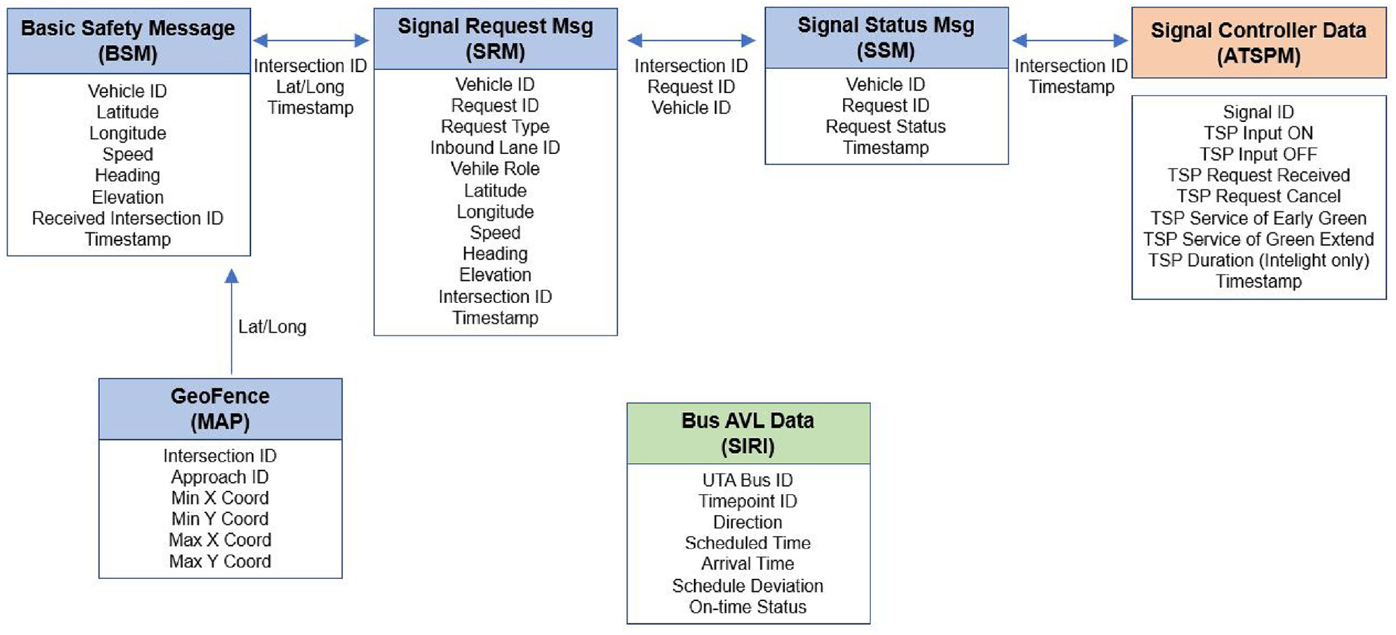
Transit signal priority (TSP) messages and data elements.
DSRC is the means by which buses on Route 217 communicate with the signal controller and request TSP. DSRC OBUs are needed on each bus and DSRC RSUs are needed at each intersection, thereby making them “equipped” buses and intersections. Of the 30 signalized intersections along the equipped portion of the route, 24 have DSRC RSUs but only 22 can serve TSP. The eight intersections that do not serve TSP are at freeway interchanges, continuous-flow intersections, and a light rail transit grade crossing.
The TSP software used is MMITSS-UT, a modified version of the MMITSS application developed for the CV Pooled Fund Study by the University of Arizona and the University of California PATH Program ( 16 ). Built into the software is a specific modification to enable conditional priority requests based on bus lateness, referred to as the requesting threshold. The TSP system uses GPS-based detection that originates from the DSRC OBU, which allows the bus to be detected without the need for any input or action by the bus operator. TSP requests are received by an intersection when the bus is within approximately 500 ft of the intersection, but this distance varies by intersection.
Analysis Methodology
The data were primarily analyzed by direction (NB and SB) and by peak period (morning and evening). These four directional-peak scenarios (AM NB; AM SB; PM NB; and PM SB) were used to analyze impacts at each timepoint individually and aggregated at the corridor level. The morning peak was defined as 06:00–09:00 and included all records that fell within that time. Likewise, the evening peak was defined as 15:00–18:00. Although data were obtained for off-peak times of day, UTA and UDOT were primarily interested in the peak periods when ridership and congestion are typically highest, so this analysis likewise focuses on the peak periods. Figure 2 is a flowchart that outlines the data sources, the analysis in which they are used, the results measured by the analysis, and the specific metrics evaluated. Following the figure, the analysis methodology for evaluating bus performance and general traffic is discussed.
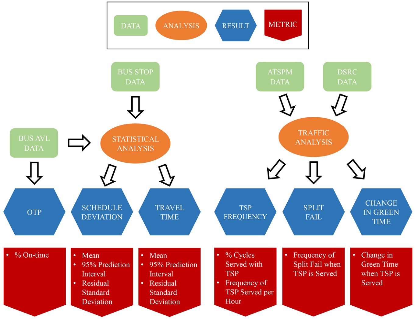
Analysis flowchart.
Bus Performance
Bus performance was evaluated primarily through three different metrics: OTP, schedule deviation, and travel time. OTP was evaluated through an observational analysis while impacts on schedule deviation and travel time were measured through a statistical analysis.
On-Time Performance
OTP, the proportion of the time that a transit system adheres to its published schedule within stated tolerances ( 4 ), was the most important metric to UTA in determining whether TSP improved bus performance. UTA indicated that a 1% improvement in OTP would be meaningful.
Statistical Analysis
A statistical analysis was performed on the data to evaluate the impact of changing the requesting threshold on schedule deviation and travel time. Specifically, analyses were performed on the mean and the 95% prediction interval. The statistical package SAS v9.4 was used to perform a mixed model multiple regression analysis blocking on hour of day and timepoint (blocking is performed to adjust for correlation in the data because of a lack of independence). Additionally, the number of times a bus had to stop to load or unload passengers was included in the model as a covariate.
After controlling for the explanatory variables: hour of day, timepoint, and number of times a bus had to stop to load or unload passengers, the schedule deviation and travel time were estimated. Estimates were created for each requesting threshold at the timepoint and corridor level for the four directional-peak scenarios.
For schedule deviation and travel time, the estimated mean was analyzed between different requesting thresholds using a one-sided t-test on the difference in means. Because multiple comparisons were made across the various requesting thresholds, a pseudo-Bonferroni adjustment was used; the improvement was statistically significant if the resulting p-value was less than or equal to 0.01.
Standard deviation was not used to estimate the range that contains 95% of the data because the data were not normally distributed. Instead, the 2.5th percentile and 97.5th percentile of the raw data values were grouped by timepoint and by directional-peak scenario to create the 95th percent prediction interval for each group. This interval was used to illustrate variability in the data and provide a range of expected values for schedule deviation and travel time.
Traffic Analysis
The traffic analysis was performed through a process developed by Avenue Consultants and guided by UDOT traffic signal engineers ( 3 ). ATSPM and DSRC data stored on UDOT servers were used in this analysis to evaluate the impact of TSP on general traffic by measuring changes in split fail and green time when TSP was granted, and the number of times TSP was requested and granted.
Split fail, which was the primary metric used to measure the impact of TSP on general traffic, occurs when the duration of green for a movement, or split, at a signalized intersection is insufficient to serve the amount of demand present ( 17 ). For this study, split failure occurred when vehicle occupancy exceeded 85% of both green time and the first 5 sec of red time. For a given conflicting phase, the frequency of split failure during the 10 min before TSP was served was compared with the frequency of split failure during the 10 min after TSP was served. If any of the conflicting phases experienced an increase in split fail from pre-TSP to post-TSP, it was determined that there was a negative impact to general traffic. Additionally, the frequency at which TSP was served was used to evaluate the overall impact on the system.
Results
It is expected that as the requesting threshold approaches zero and TSP is requested and consequently served more often, there will be greater positive impacts on bus performance and greater negative impacts on general traffic. Indeed, the percentage of records where the schedule deviation of equipped buses exceeded the requesting threshold was 22.6% for the 3-min threshold, 31.7% for the 2-min threshold, and 92.9% for the 0-min threshold. Therefore, the purpose of this research is to determine the optimal requesting threshold to balance the positive impacts of TSP on bus performance with the negative impacts on general traffic. The following sections contain the results of the bus performance and general traffic analyses. More details on the research presented in this paper can be found in the literature ( 18 ).
Bus Performance
This section contains the results of the bus performance analysis by evaluating OTP, mean schedule deviation, and the 95% prediction interval for schedule deviation and travel time.
On-Time Performance
The data show that as the requesting threshold approaches zero, OTP increases, with the evening NB being the only exception. On average, when data from all directional-peak scenarios are combined, OTP increased 2.0% when the requesting threshold changed from 3 min to 2 min, and 2.5% when the requesting threshold changed from 2 min to 0 min. Figure 3 contains the results of the corridor-level OTP analysis.
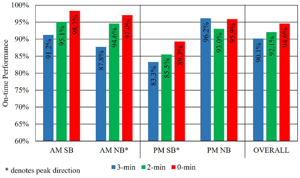
Corridor-level on-time performance.
Schedule Deviation: Mean
The statistical model was used to estimate the mean schedule deviation for each directional-peak scenario at the timepoint-level, corridor-level, and overall. The overall results combine data from all directional-peak scenarios. Figure 4 contains estimates of the mean schedule deviation at the corridor-level and overall.

Corridor-level mean schedule deviation.
The comparison of means between two requesting thresholds was performed through a one-sided t-test, which measures whether there is evidence that mean schedule deviation decreases (improves) as the requesting threshold approaches zero. The corridor-level p-values from the difference in means statistical analysis are displayed in Table 1 and are organized by directional-peak scenario and comparison pair. The shaded cells in Table 1 emphasize p-values less than 0.01 (the pseudo-Bonferroni adjustment) and indicate that a statistically significant improvement in mean schedule deviation exists for the given comparison pair and directional-peak scenario according to the null hypothesis.
Corridor-Level Schedule Deviation Difference in Means p-Values
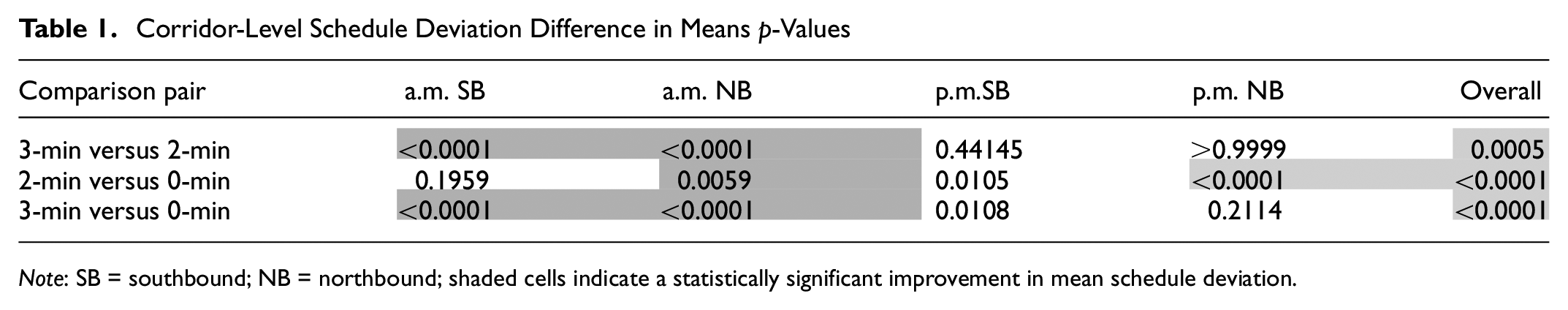
Note: SB = southbound; NB = northbound; shaded cells indicate a statistically significant improvement in mean schedule deviation.
Practically the same trends are present for mean schedule deviation as were observed for OTP. Anomalies are once again seen in the evening NB, but for the remaining three directional-peak scenarios, the corridor-level mean schedule deviation always improved as the requesting threshold changed from 3 min to 2 min, and from 2 min to 0 min.
Despite the evening NB anomalies, the overall mean schedule deviation drops from 123.4 sec at the 3-min threshold to 107.5 sec at the 2-min threshold (p = 0.0005), and from 107.5 sec at the 2-min threshold to 86.6 sec at the 0-min threshold (p < 0.0001). On average, mean schedule deviation improved 18.4 sec each time the requesting threshold changed from 3 min to 2 min, and from 2 min to 0 min. Although there is convincing evidence overall that mean schedule deviation improves (decreases) as the requesting threshold approaches zero, this was not the case in every directional-peak scenario. In fact, it was only the morning peak period where significant improvements occurred consistently.
Schedule Deviation: 95% Prediction Interval
The 95% prediction interval is the range of expected values based on the value of the 2.5th and 97.5th percentiles, thus representing the middle 95% of data. The magnitude of the 95% prediction interval is determined by calculating the difference in seconds between the values of the 97.5th and 2.5th percentiles. As the magnitude of the 95% prediction interval increases, variability in the data increases. Figure 5 contains the corridor-level and overall results of the 95% prediction interval for schedule deviation. The trendline for median schedule deviation values represented in the figure decrease between 17 sec and 33 sec each time the requesting threshold changes from 3, to 2, to 0 min.

Corridor-level schedule deviation 95% prediction interval.
Additionally, it is important to note that along with improvements for median schedule deviation, the upper bound of the 95th percent prediction interval (the 97.5th percentile value) experienced considerably greater improvements. In the morning NB scenario, for instance, all median values are within 65 sec of each other while the 97.5th percentile values have a range of 176 sec (486 sec for the 3-min threshold and 310 sec for the 0-min threshold).
Travel Time: 95% Prediction Interval
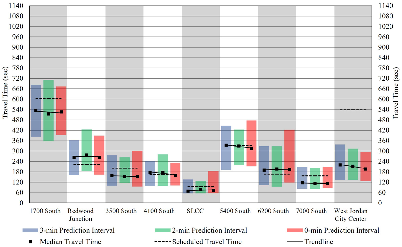
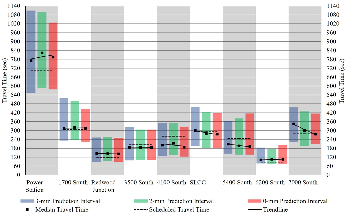
Figure 6 through Figure 9 contain graphs of the travel time 95% prediction interval for each direction-peak scenario. Also plotted is the median travel time, a trendline for the median travel time at each timepoint, and the scheduled travel time.

Morning northbound travel time 95% prediction interval.
Morning southbound travel time 95% prediction interval.
Evening northbound travel time 95% prediction interval.
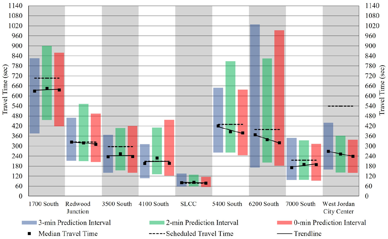
Evening southbound travel time 95% prediction interval.
Several inferences can be drawn from displaying the travel time data in this manner. First, the slope of the trendline is negative at 27 of 36 timepoints (9 timepoints for each of the four directional-peak scenarios), which suggests that as the requesting threshold approaches zero, travel time decreases. As the requesting threshold changed from 3, to 2, to 0 min, each change resulted in an average decrease in travel time of 7.5 sec per timepoint.
While the median travel time usually decreased as the requesting threshold approached zero, there is not a clear change in the magnitude of the 95% prediction interval, or a suggested change in variability. Indeed, the average magnitudes of the 95% prediction interval for the 3-, 2-, and 0-min requesting threshold are respectively 257, 243, and 244 sec.
Dwell Time
An observed negative impact on buses that is theorized to be attributed to TSP is increased dwell time at timepoints because of holding buses that are early, a UTA operational strategy to improve schedule adherence. The TCQSM defines dwell time as “the time spent at a stop or station serving passenger movements, including the time required to open and close the doors. Time spent at a stop for any other reason, such as waiting for a traffic signal, waiting for another transit vehicle to move, or waiting for late-arriving passengers is considered delay and is not counted as part of dwell time” ( 4 ). Likewise, the Highway Capacity Manual (HCM) defines dwell time as “the sum of the time required to serve passengers at a transit stop and the time required to open and close the vehicle doors” ( 19 ). There are several contributing factors to dwell time, including (but not limited to) boarding and alighting volumes, fare payment method, vehicle type and size, number of passengers with wheelchairs or bicycles, and operator interactions with passengers (e.g., answering questions or fare disputes) ( 4 ).
Discussions with UTA personnel revealed that UTA records “dwell time” as the time from which a bus enters a geofence around a stop to the time at which it leaves the geofence. This makes it impossible to determine how much of the recorded time was actual dwell time, as defined by the TCQSM and the HCM, delay, versus because of the holding of early buses.
While it is reasonable that actual dwell time or other sources of delay could be considered constant for each requesting threshold, it was determined to be unreasonable to consider holding time constant; buses receiving TSP at the 0-min threshold are more likely to be early at the subsequent timepoint and hold than buses that receive TSP at the 3-min requesting threshold. Therefore, it would be expected that as the requesting threshold approaches zero, the recorded dwell time would increase because of TSP helping the bus so much that it becomes early and needs to hold at subsequent timepoints. Indeed, this expectation is observed with average cumulative dwell time at the 3-, 2-, and 0-min thresholds being 449, 464, and 525 sec, respectively. This suggests that some of the benefits from TSP are lost because of the holding strategy, especially when the 0-min requesting threshold was implemented.
Traffic Analysis
Contrary to how bus performance was analyzed, the traffic analysis evaluates the impact of changing the requesting threshold by morning and evening peak, thereby combining instances in which TSP was served for NB and SB buses. This section contains the results of the analyses for the frequency at which TSP is served and split fail.
TSP Frequency
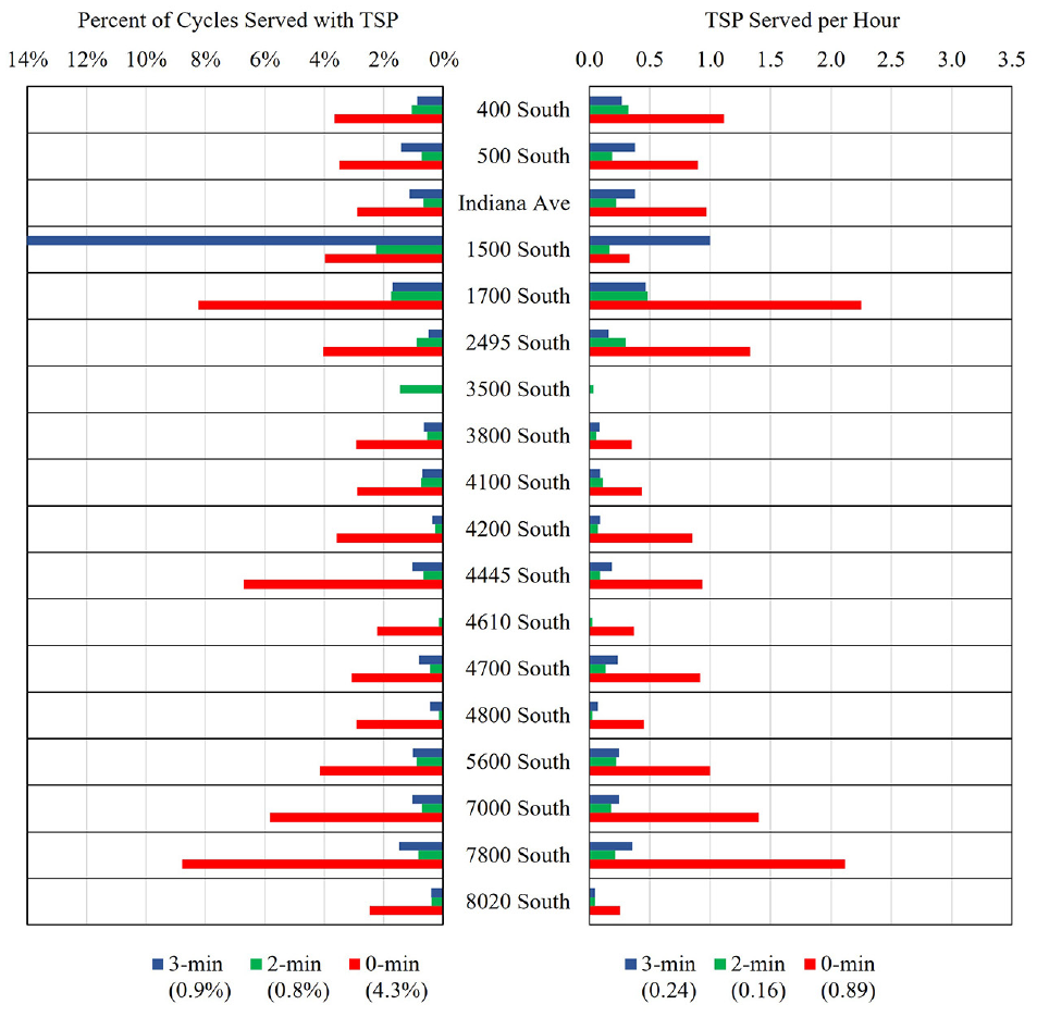
For all equipped intersections capable of serving TSP, the percent of cycles served with TSP is displayed in Figure 10a and the frequency of TSP served per hour is shown in Figure 10b, with averages by peak period shown in parenthesis along the x-axis. It is clear that the 2-min and 3-min requesting thresholds are very similar with respect to the percent of cycles that are affected (numerical difference of 0.2 %) and how many times per hour TSP is served (difference of 0.03 times per hour). However, the results for both metrics are much higher for the 0-min threshold. A comparison of the average values of the 2-min and 3-min thresholds with the 0-min requesting threshold results provides the following insights: for the percent of cycles served with TSP, the 0-min threshold is 307% higher; and for the number of times TSP is served per hour the 0-min threshold is 284% higher. Figures 11 and 12 contain the intersection-level results of the percent of cycles served with TSP and the frequency of TSP served per hour for the morning and evening peaks, respectively.
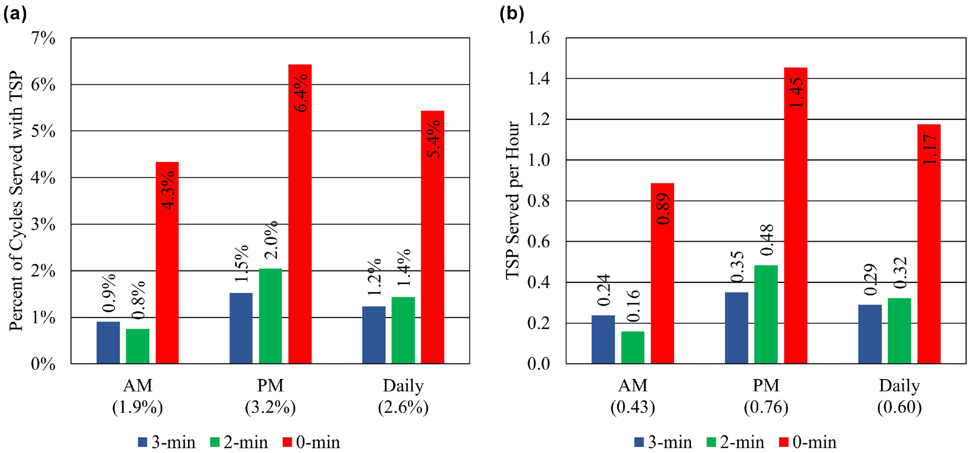
Corridor-level: (a) percent of cycles served with transit signal priority (TSP) and (b) frequency of TSP served per hour.
Morning peak intersection-level frequency of transit signal priority (TSP) served.

Evening peak intersection-level frequency of transit signal priority (TSP) served.
Split Fail
Split fail occurs when the duration of green for a movement at a signalized intersection is insufficient to serve the amount of demand present. It is determined that split failure has occurred when vehicle occupancy exceeded 85% of both green time and the first 5 sec of red time. The figures in this section represent how split fail was affected when TSP was served. Figure 13 shows the corridor-level results of the split fail analysis with the intersection-level results shown in Figure 14 for the morning and evening peaks.
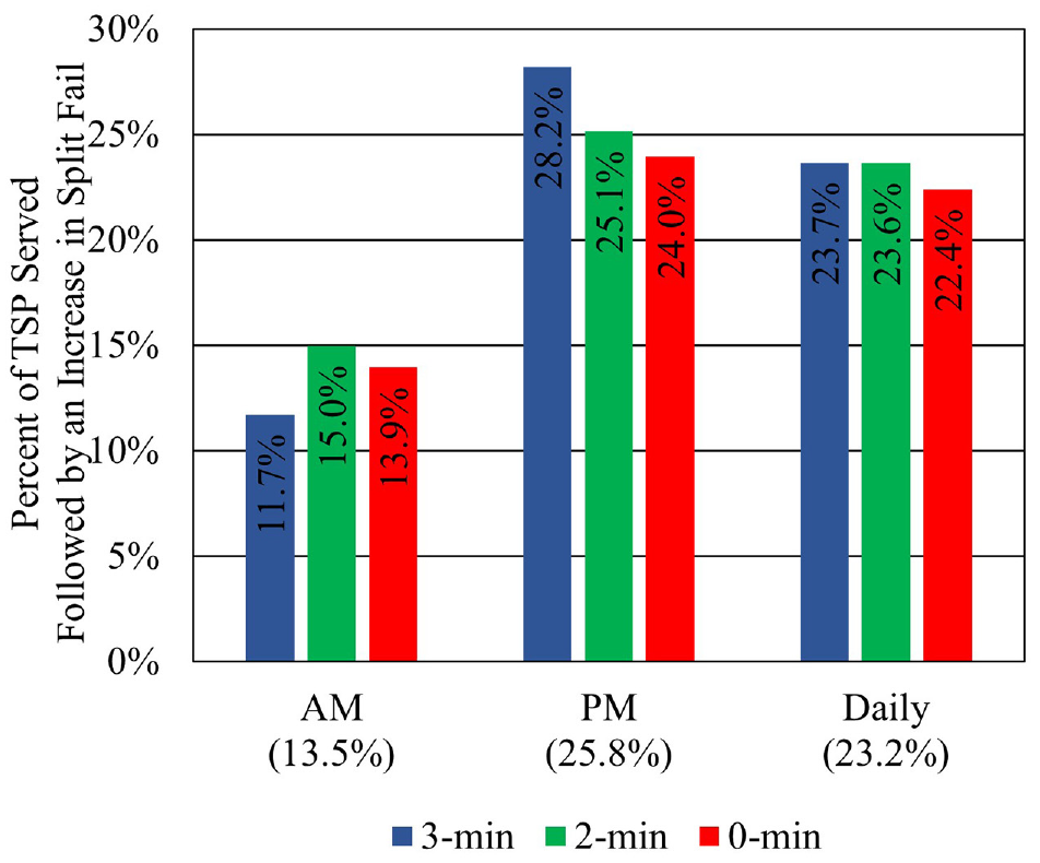
Corridor-level split fail results.
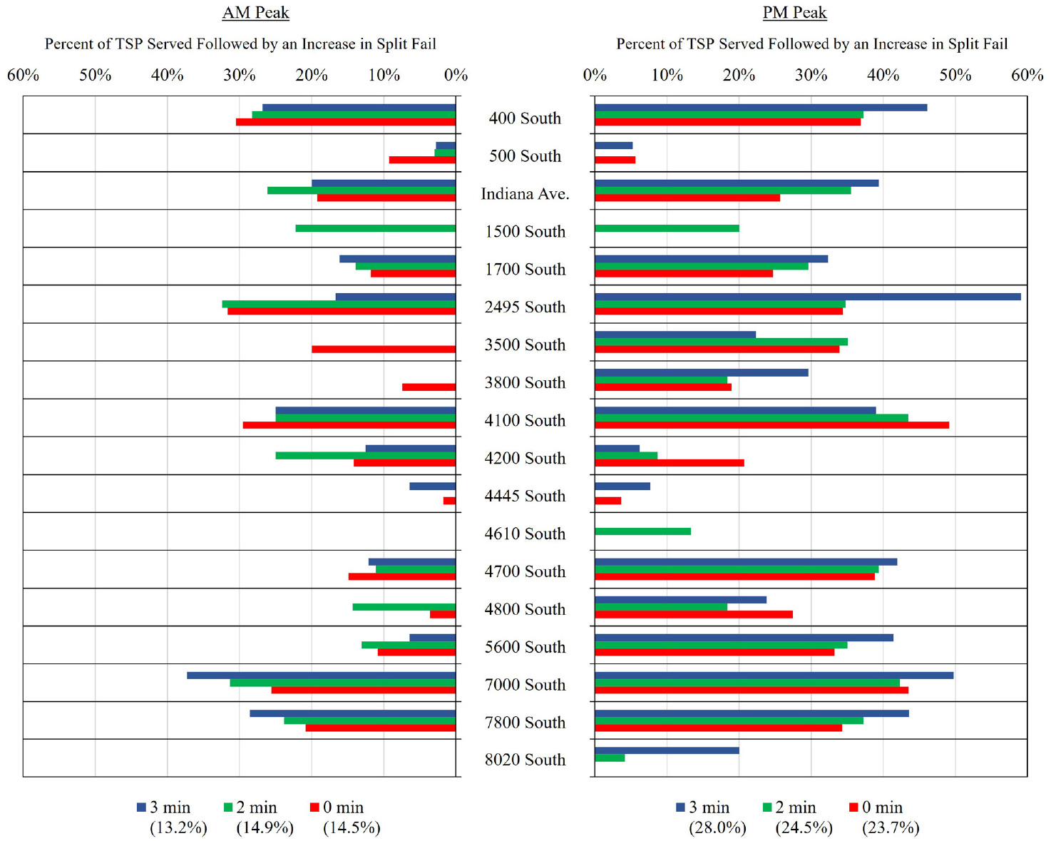
Intersection-level split fail results for: (left) the morning peak, and (right) the evening peak.
It was unexpected to see that the occurrence of split failure decreased (improved) as the requesting threshold approached zero. Although the cause of this phenomena was not verified, the research team believes that this occurred because when TSP was served at the 3-min threshold, traffic was more congested. That is not to say that traffic was inherently worse during the weeks that the 3-min data were collected, but rather because the bus was 3 min behind schedule it was likely that traffic was worse.
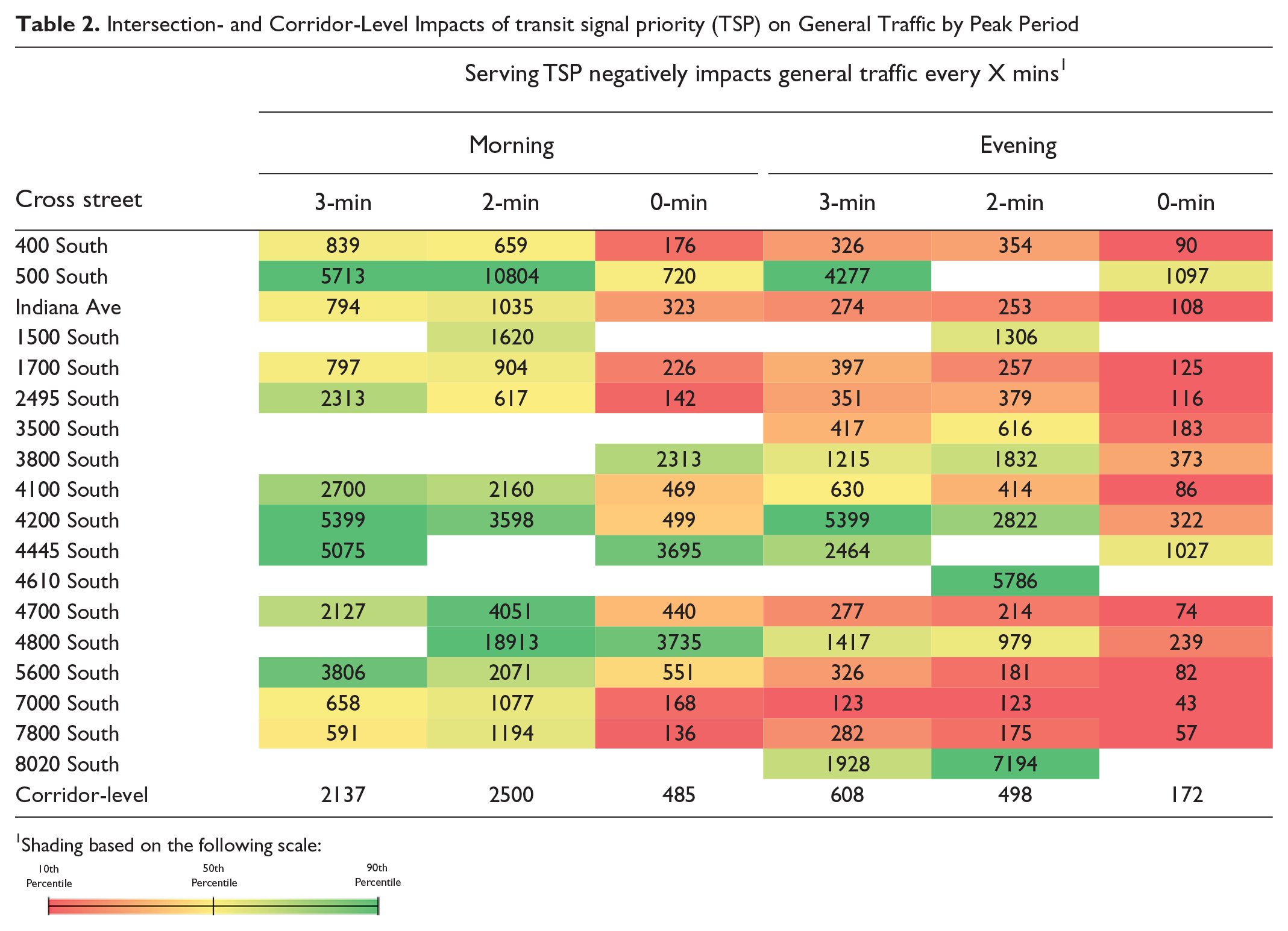
The frequency at which TSP is served was multiplied by the percent of TSP served followed by an increase in the split fail metric to obtain the frequency at which it is suggested that TSP negatively impacted general traffic. Table 2 contains the results of this analysis at the corridor- and intersection-level by peak period and indicates that inconsequential negative impacts to general traffic occur when TSP is served.
Intersection- and Corridor-Level Impacts of transit signal priority (TSP) on General Traffic by Peak Period
Shading based on the following scale:
For the 3-min requesting threshold during the morning peak, for example, TSP was served an average of 0.24 times per hour (see Figure 10b) while an average of 11.7% of those events resulted in an increase in split fail, or negative impacts to general traffic (see Figure 13). Multiplying the two together suggests that, on average, TSP causes negative impacts to general traffic 0.028 times per hour, or once every 2,137 min. The evening peak during the 0-min requesting threshold had the greatest impact with TSP negatively impacting general traffic once every 172 min, or approximately once every 3 hours.
Table 2 is overlaid with a three-color scale heatmap where the green, yellow, and red shadings correspond to the 90th, 50th, and 10th percentile of all values in the table. This means that dark red shading highlights lower values, which indicates that traffic is negatively affected at a higher frequency, and dark green indicates the intersections where there is the least potential for traffic to be negatively affected. The white areas indicate scenarios where no increase in split failure was recorded during the study period.
The intersection and scenario with the greatest suggested impact on general traffic is 7000 South during the evening peak at the 0-min threshold, which indicates that TSP negatively impacts traffic once every 43 min. The heatmap also illustrates that negative impacts on general traffic occurred more frequently during the 0-min threshold and during the evening peak.
Conclusion
After implementing TSP along UTA Route 217 in November 2017, research determined that equipped buses capable of requesting TSP were on time 3% more often than non-equipped buses. Following implementation, optimization was needed to further improve the effectiveness and efficiency of the operation. This research optimizes the operation outside of a simulation and through field data exclusively by performing a sensitivity analysis of the TSP requesting threshold parameter. The requesting threshold is the point at which TSP is requested and is defined by how far behind schedule the transit vehicle must be to request TSP. For this research, 3-, 2-, and 0-min requesting thresholds were evaluated.
It is expected that as the requesting threshold approaches zero and TSP is requested and consequently served more often, there will be greater positive impacts on bus performance and greater negative impacts on general traffic. Therefore, the purpose of this research was to determine the optimal requesting threshold to balance the positive impacts of TSP on bus performance with the negative impacts on general traffic. The results of this research will improve the effectiveness and efficiency of TSP on Route 217, help other agencies understand the impact of changing the requesting threshold for their TSP deployments, and help UDOT and UTA meet their goal of improving mobility through optimization and innovation.
The analysis concludes that as the requesting threshold approaches zero, OTP, schedule deviation, and travel time improve, while general traffic is only negligibly impacted. For Route 217 OTP, as the requesting threshold changed from 3 min to 2 min and from 2 min to 0 min, OTP improved 2.0% and 2.5%, respectively. For schedule deviation, as the requesting threshold changed from 3 min to 2 min and from 2 min to 0 min, mean schedule deviation improved 15.9 sec (p = 0.0005) and 20.9 sec (p < 0.0001), respectively. The improvements to Route 217 travel time were observational and showed that median travel time between timepoints decreased an average of 7.5 sec each time the requesting threshold changed from 3-, to 2-, to 0-min.
The traffic analysis shows that negative impacts on general traffic rarely follow the serving of TSP. Even though serving TSP at the 0-min threshold impacted general traffic three to four times as often as the 2-min threshold, negative impacts were infrequent and were observed a maximum of once every 43 min.
Footnotes
Acknowledgements
Appreciation is specifically extended to the following individuals: from UDOT, Blaine Leonard, Jamie Mackey, Peter Jager, Vincent Liu, Devin Squires, and Matt Luker; from Avenue Consultants, Shawn Larson; from UTA, Tom McMahon, Scott Bingham, Lorin Simpson, Thad Golding, Vincent Nguyen, Jordan Eves, Casey Brock, John Hansen, Dan Riley, and Mike Sprouse; from The Narwhal Group, Jonny Turner and Ralph Koeber; and from BYU, Mason Shoaf, Adrian Moreno, Jordi Berrett, Hayden Andersen, Shanisa Butt, and Michael Adamson.
Author Contributions
The authors confirm contribution to the paper as follows: study conception and design: M. Sheffield, G. Schultz, D. Bassett, and D. Eggett; data collection: M. Sheffield; analysis and interpretation of results: M. Sheffield, G. Schultz, D. Bassett, and D. Eggett; draft manuscript preparation: M. Sheffield, G. Schultz. All authors reviewed the results and approved the final version of the manuscript.
Declaration of Conflicting Interests
The author(s) declared no potential conflicts of interest with respect to the research, authorship, and/or publication of this article.
Funding
The author(s) disclosed receipt of the following financial support for the research, authorship, and/or publication of this article: This research was managed and funded by the Utah Department of Transportation under the direction of Blaine Leonard and was performed in cooperation with the Utah Transit Authority (UTA) and Brigham Young University (BYU).
The authors alone are responsible for the preparation and accuracy of the information, data, analysis, discussions, recommendations, and conclusions presented here. The contents do not necessarily reflect the views, opinions, endorsements, or policies of the Utah Department of Transportation or the US Department of Transportation. The Utah Department of Transportation makes no representation or warranty of any kind, and assumes no liability therefore.