Dynamically Collected Local Density using Low-Cost Lidar and its Application to Traffic Models

Abstract

This article demonstrates the use of traffic density observations collected dynamically in the vicinity of probe vehicles. Fixed position sensors cannot capture the longitudinal evolution of local traffic density in the corridor. In this research, dynamic traffic density observations were collected in a naturalistic driving setting that was free of any controlled experiment biases. Speed from global positioning system and space headway from a light detection and ranging module was collected on one arterial and one freeway segment, 2 and 4 mi long, respectively. The combined data frequency was approximately 3 Hz. Space headway was used to estimate the local density and consequently to identify the density of a specific location in a corridor. Besides, driver behavior was characterized using the relationship between instantaneous speed and local density under different regimes of the Wiedemann car-following model. Macroscopic traffic stream models were used to investigate the relationship between dynamically collected instantaneous speed and local density. Using the longitudinal evolution of density, precise local density across the corridor can be obtained along with the leader and follower trajectories. A method to identify driver behavior across density ranges was developed for different facility types using a microscopic relationship between instantaneous speed and local density. Overall driving behavior on the freeway segment can be represented by translating the instantaneous speed and local density relationship to macroscopic stream models.

One of the common methods of collecting traffic flow and vehicle volume data on a segment is through static or stationary infrastructure sensors. Examples of those are stationary video cameras or vehicle counting sensors like the remote traffic microwave sensor (RTMS) ( 1 ). These methods, however, lack variation in space over the segment as the sensors are fixed to a location and the collected data are usually averaged out to estimate the information about the entire segment. This is often the reason macroscopic models use average speed and average density. Also, installations and reinstallations of these stationary sensors in different locations are expensive and difficult to maintain ( 2 ).

An alternative solution to collect data cost-effectively would be through a dynamic method where the sensor is in motion. Some researchers have used devices that collect vehicular speed data from the on-board diagnostics (OBD) port ( 3 ), and some have used global positioning system (GPS) devices to log vehicular speed and positional data from probe vehicles ( 4 ). However, these dynamic methods of data collection cannot report vehicle volume or occupancy information.

A promising method would be to combine one of the abovementioned approaches, that is, using GPS or OBD data, to collect vehicular speed along with a sensor that collects spatial headway information from a moving vehicle. This can be achieved by using light detection and ranging (lidar) or radio detection and ranging (radar). Similar set-ups are found on commercially available autonomous vehicles (AV). Nowadays, some vehicles are equipped with a variety of sensors to provide different forms of information to the driver. Lidars are used to detect and measure the distance of objects or vehicles from an AV ( 5 ) and GPS modules are used in the in-built navigation systems for positional data. Most 3-D lidar and radar modules are expensive. However, this study used a low-cost approach to collect spatial headway data using a 2-D lidar ( 6 ). Despite being low-cost, 2-D lidar has a high precision rate and a strong resistance to interference. It is also robust to illumination variations ( 7 ). However, this paper does not intend to advise on the use of one type of sensor over the other.

From instantaneous spatial headway captured, “local density” can be calculated, along with the characterization of the entire lead vehicle trajectory while that vehicle is in range. The local density is generated based on the driver’s reactions to the leading vehicle, that is, the dynamic data collected pertaining to the driver of the following (equipped) vehicle across the corridor. The advantage of this naturalistic approach is that the information is collected without any bias or any controlled conditions.

A review of past studies related to static and dynamic sensors is discussed in the literature review. Following the literature review, the methods and the scenarios used to collect the data, along with the formulas used to estimate various parameters and route characteristics, are explained in the methodology. The results section consists of three methods of data investigation. Finally, the key findings of this paper are summarized in the last section.

Literature Review

Various methods using static sensors have been employed to collect microscopic information, such as speed and headway, and macroscopic information, such as vehicle occupancy and vehicle flows. One such method was to use an offline image processing tool to classify vehicles in a mixed traffic scenario and gather microscopic information, such as speed and headway, and macroscopic characteristics, such as vehicle trajectories, vehicle occupancy, and so on ( 8 ). The drawbacks of similar systems are that the area covered by theses sensors is only hundreds of feet wide. As such, they lack spatial variation over the segment and the installation and maintenance costs would also be expensive. The challenges faced in using these non-intrusive technologies include: restrictive installation requirements; sensors being sensitive to environmental conditions, which severely affect areas where continuous data is needed; and their relatively high costs ( 9 – 11 ). Dynamic data-driven applications are, therefore, the way to move forward with the advancements in technology ( 12 ).

One of the alternative solutions for static data collection was the data logging from the OBD port. The OBD port provides a lot of vehicular information like speed, acceleration, engine RPM, and so on. A variety of research has been performed using OBD data to evaluate driving behavior ( 13 ), remote logging of vehicular data ( 14 ), and so on. Like the speed data from the OBD port, the GPS devices are used to capture vehicular speed through satellites. Research has shown that using GPS traces is a cost-effective and reliable way to record speed data ( 15 ). GPS data have been used to model low-speed urban roads based on operating speed ( 16 ). Alternatively, apart from collecting speed data, researchers have used positional data from the GPS to calculate the headway of vehicles ( 17 ); however, the disadvantage of this system is that it depends on the leading vehicle having the GPS device as well. Interestingly, the use of a lidar/radar along with the GPS will remove the dependency of every vehicle to have the GPS device. Lidar and radar have their own set of pros and cons, yet those are the two most widely used devices to measure spatial headway in cars ( 18 ).

The car is assumed to be following when the driver is unable to drive at the posted speed and is constrained by the leading vehicle ( 19 ). The car-following model we are using is a psycho-physical model called a Wiedemann model adopted by VISSIM. We have used an enhanced version of the 1974 model, proposed by Wiedemann and Reiter ( 20 ). The Wiedemann model, a microscopic car-following model, represents a single driver’s behavior and uses dynamic information such as spatial headway, speed of the follower, and speed of the leader vehicle. In the Wiedemann car-following model, the thresholds are defined for every speed, so it helps to identify the driving behavior at different speeds ( 21 ). Through this model, each spatial headway data point is categorized into a regime.

Various macroscopic models, such as Greenshields, Greenberg, modified Greenberg, and so forth, are used for investigating the quality and closeness of the speed-density data. These models are usually fitted to data that are collected using static sensors over time at a given location with temporal variation; however, these models lack variation in space over the segment. Throughout this paper, we investigate how these models would represent the dynamic data which has less temporal variation and more spatial variation over the segment.

It can be gleaned from the reviewed literature that some systems capture speed and vehicle occupancy from static locations; however, most systems are incapable of capturing the evolution of traffic density. Some dynamic systems like GPS or OBD devices capture speed data; however, those sensors do not capture density data. Methods used to collect speed and density data from the GPS require a controlled environment and are dependent on other vehicles to house similar data-capturing devices to obtain speed and density data. In contrast, this paper uses the data captured in an independent, naturalistic, and dynamic manner and also answers questions such as: (a) What is the need for density data through dynamic data collection? (b) How does classifying speed-density data into regimes help in characterizing driving behavior? and (c) Can some of the existing macroscopic models represent the dynamic data?

The research is not intended to represent all vehicles in one lane or multiple lanes in the corridor. The current scope of this research is limited to the study of the behavioral characteristics of a single driver in the equipped vehicle, analyzing speed-local density at the micro level, and proposing methodology to assign local density information to a driver. We have performed three types of analysis using the collected data: (a) trip characterization using density data; (b) classification of the differential speed-local density domain into different car-following regimes; and (c) a comparison of various traditional macroscopic models with the collected speed-local density data. The data streams generated in this work resemble those likely to be produced by autonomous and connected vehicles, thus providing a preview of possible applications of such data for enhanced mobility and safety purposes. If a segment needs to be equipped with static sensors, both the legal administrative process and coordinating with various departments to install the devices are time-consuming tasks. On the contrary, data from probe vehicles can be retrieved within days. Agencies have started using probe data for origin–destination studies and this research is headed in the same direction.

Methodology

In this section, the vehicle hardware components used for data collection are first described. The design of the naturalistic driving experiments on both arterial and freeway sections is explained next. This section also presents how the data are being used for numerical analysis of the local density data, classification of the speed-local density domain by car-following regime, and for comparing against various macroscopic models.

Instrumentation and data collection

A probe vehicle equipped with a system comprising a low-cost 2-D lidar module, GPS, real-time clock, and a camera was used. All these components were connected to an Arduino device that synchronizes the data and sends it to a “raspberry pi” to store the information. The lidar unit, which has a coverage of 40 m, was mounted to the hood of the vehicle (Figure 1b) and the remaining devices were placed inside the vehicle. The devices were powered by a 12V DC output from the car. The set-up and system details can be found in this study ( 6 ).

Figure 1.

(a) System architecture and processes ( 6 ); (b) lidar module mounting ( 6 ); (c) the arterial route; and (d) the freeway route.

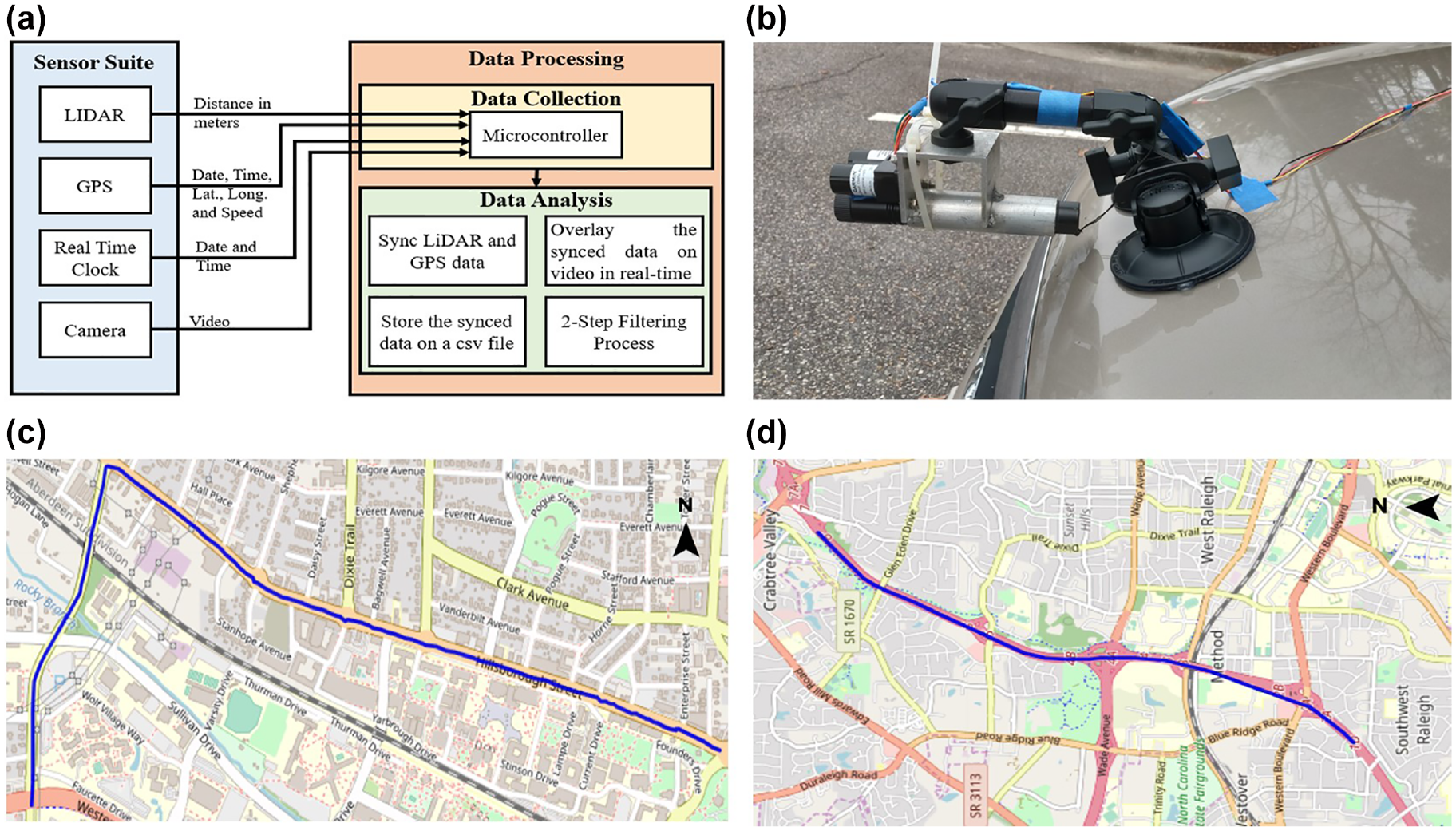
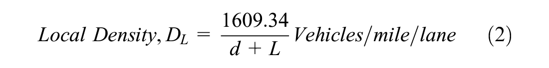
The data were collected by the instrumented vehicle naturalistically along two routes. The chosen routes are an arterial segment and a freeway segment as shown in Figure 1, c and d. The arterial route was northbound on Gorman Street followed by eastbound on Hillsborough Street in Raleigh, NC. The freeway route was southbound on Interstate-440 from Exit 7 to Exit 1D. In both routes, two sets of data were collected, one in the a.m. off-peak and one in the p.m. peak, resulting in four scenarios in total. The collected data consisted of timestamps, speed (mph), headway (in meters), and subject vehicle positional data such as latitude and longitude. The time, speed, and headway data were overlaid on the video, which was used as a reference to understand and confirm the results.

Calculations and Estimations

Important information that was not measured in real-time would be the speed of the leading vehicle, which is estimated using the following formula

Speed of the leader, v_{l} = v_{f} + \frac{Δ d}{Δ t}, mile / hour

(1)

where

$v_{f}$ is the instantaneous speed of the follower,

$Δ d$ is the difference in the gap (rear bumper of the leading vehicle to the front bumper of the following vehicle), and

$Δ t$ is the difference between time instants.

The data collected can be visualized in various forms.

The spatial headway data give us information about the car-following distance maintained by the follower at every instant, from which the average spatial distance over the segment can be measured.

Since the speed of the follower was known at any point on the route, it can be compared with aggregated probe data collected by third-party companies such as HERE and INRIX. Here we compare the instantaneous speed of the follower along the segment from the GPS device with the data obtained from the Regional Integrated Transportation Information System (RITIS) ( 22 ). We can also compare these speeds with the estimated speed of the leading vehicle. The speed of the leader data was available only when there were valid spatial headway data points of the leading vehicle, that is, when the vehicle was in range and its data were not filtered out because of sensor errors ( 6 ).

Like the speed of the leader vehicle, the local density was also estimated using the captured information with the formula as;

Local Density, D_{L} = \frac{1609.34}{d + L} Vehicles / mile / lane

(2)

where d is the gap (rear bumper of the leading vehicle to front bumper of the following vehicle) in meters and L is the length of the following (equipped) vehicle in meters. A minimum $D_{L}$ of 35 vpl can be achieved with d as 40 m (maximum range of lidar sensor) and L as 6 m. A driver’s car-following behavior is more critical at densities near the breakpoint density. According to HCM6, basic freeway segments have a breakpoint density of 45 passenger car per mile per lane ( 23 ). Therefore, a limit of 35 vehicles per mile per lane will capture the breakpoint conditions. Using $D_{L}$ , we can understand the local density distribution across the segment, unlike the stationary sensors which capture information only for a small portion of a segment. Based on the local density variation, we can understand the driver’s behavior pertaining to the environment and the traffic conditions.

To implement the 1992 Wiedemann-Reiter car-following model we calculate two important parameters ( 19 ):

Space Headway, Δ x = d + L, meters

(3)

where d is the gap (rear bumper of the leading vehicle to front bumper of the following vehicle) in meters, and L is the length of the leading vehicle in meters, and the difference in speed is;

Δ v = v_{f} - v_{l}, mile / hour

(4)

where $v_{f}$ is the instantaneous speed of the follower, and $v_{l}$ is the speed of the leader in mph.

Wiedemann Car-Following Regimes

The Wiedemann car-following model is the largest parameterized model when compared with similar car-following models ( 19 ). So, using the above two parameters, $Δ v and Δ x$ , along with certain calibration parameters, the thresholds for the Wiedemann car-following model were defined. These thresholds help in characterizing the driver’s driving regimes. As shown in Figure 2 there are in total six thresholds defined for this model, namely:

AX: the desired distance for stationary vehicles;

ABX: the threshold for desired following distance for low speeds. The Emergency regime occurs at low speeds when the speed difference is positive, that is, the speed of follower is greater than the speed of leader and vice versa would be the high-density regime;

SDX: the threshold where the following vehicle falls far too behind the leading vehicle;

SDV: the threshold where the following vehicle is approaching a slower leading vehicle (approaching regime);

CLDV: the threshold where the following vehicle must decelerate to avoid an accident with the leading vehicle (closing-in regime); and

OPDV: the threshold for small speed variations for increasing distances (free driving regime).

Figure 2.

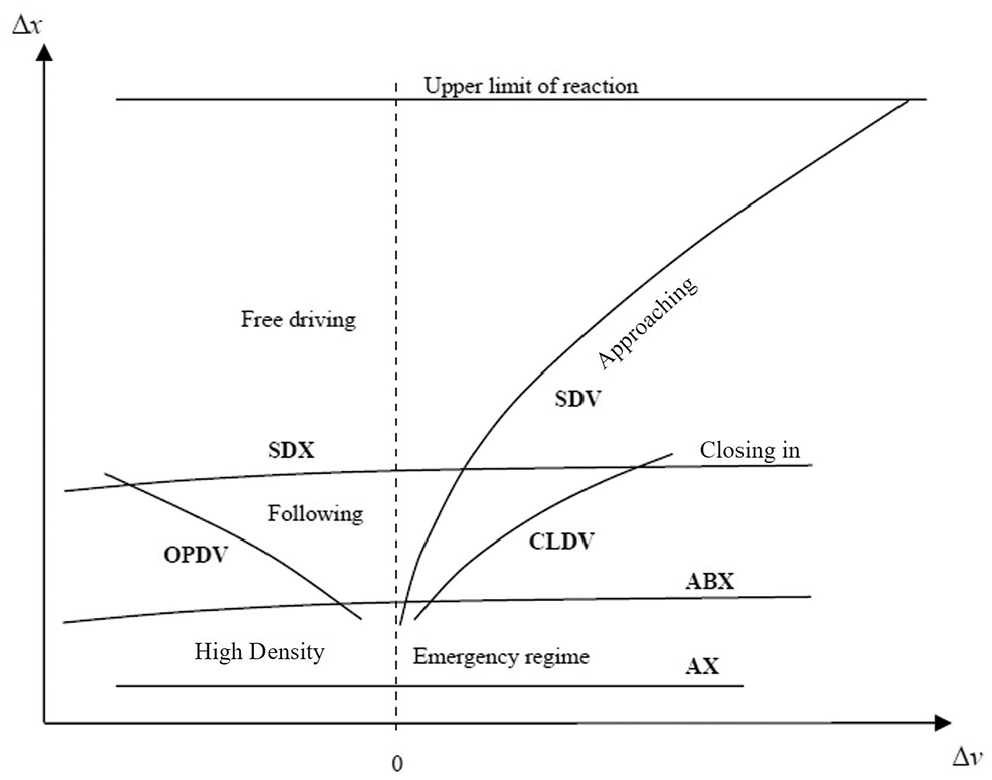
Regime thresholds of the Wiedemann model ( 19 ).

AX would be the desired distance between two stationary vehicles:

AX = L_{n - 1} + AXadd + RND 1 n * AXmult

(5)

where $AXadd and AXmult$ are calibration parameters, whose default values are 1.25 and 2.5 respectively ( 19 ). ABX is the desired distance between the leader and follower at low speed differences:

ABX = AX + BX

(6)

BX = (BXadd + BXmult * RND 1 n) * \sqrt{v}

(7)

v = {v_{l} : ν_{f} > ν_{l}, v_{f} : ν_{l} \geq ν_{f}}

(8)

where $BXadd and BXmult$ are calibration parameters, whose default values are 2 and 1 respectively ( 19 ). The maximum distance maintained by the follower in a car-following scenario is defined as SDX:

SDX = AX + EX * BX

(9)

EX = EXadd + EXmult * (NRND - RND 2_{n})

(10)

where $EXadd and EXmult$ are calibration parameters, whose default values are 1.5 and 0.55 ( 19 ). SDV is the point where the driver realizes they are approaching a slower vehicle:

SDV = {(\frac{Δ x - L_{n - 1} - AX}{CX})}^{2}

(11)

CX = CXconst * (CXadd + CXmult * (RND 1 n + RND 2 n))

(12)

where $CXconst, CXadd and CXmult$ are calibration parameters; CX is rounded to 40 ( 19 ). CLDV is the point where the driver realizes they are closing in on a slower vehicle and must decelerate to avoid a collision:

CLDV = SDV * E X^{2}

(13)

Finally, we have the OPDV threshold where the driver realizes that their speed is not constrained by the leading vehicle,

OPDV = CLDV * (- OPDVadd - OPDVmult * NRND)

(14)

where $OPDVadd and OPDVmult$ are calibration parameters whose default values are 1.5 and 1.5 respectively ( 19 ). There are three normally distributed driver parameters namely, $NRND, RND 1_{n} and RND 2_{n}$ , whose values are $N (0.5, 0.15)$ ( 19 ). For all calculations, the mean value of 0.5 has been used.

With the local density estimated, instantaneous speed, local density plots, and Wiedemann regimes can be compared to understand driving behavior.

Macroscopic Traffic Flow Models

Macroscopic traffic stream models like Greenshields and modified Greenberg were used to investigate the quality of the dynamic data from the freeway segment based on their best-fit parameters. In the Greenshields model, the speed-density relationship is expressed as ( 24 );

u = u_{f} (1 - \frac{k}{k_{j}})

(15)

where $u, u_{f}, k$ and $k_{j}$ are the speed, free-flow speed, density, and jam density. Unlike Greenshields, which is a single regime model, modified Greenberg is a multi-regime model where the data are categorized into the free-flow and congested regime. The speed-density relation for speeds above the free-flow speed $u_{f}$ is expressed as ( 24 ):

u = u_{m} * \ln (\frac{kj}{k})

(16)

where $u, u_{m}, k$ and $k_{j}$ are the speed, optimum speed, density, and jam density.

In the following results section, we discuss the inferences made from the data in detail through various visualizations using the estimated parameters, Wiedemann car-following regimes, and macroscopic models.

Results

This section discusses the trip characteristics from the three scenarios: use of local density data, the inference from the instantaneous speed/local density relation with Wiedemann car following, and the comparison of standard steady-state macroscopic models with the instantaneous speed/local density data.

Trip Characteristics and Inferences

As mentioned earlier, various areas of information such as headway, speed of follower, speed of the leader, average route speed obtained from RITIS, and Wiedemann car-following models are visualized to understand the actual traffic condition at the time of capturing.

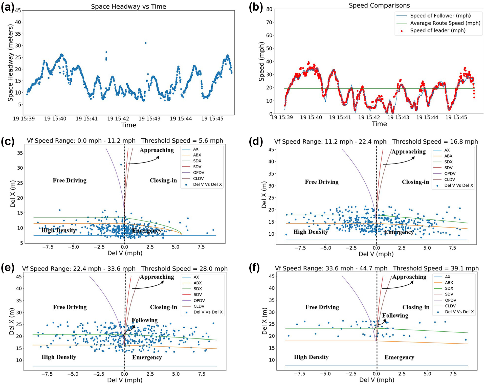
Figure 3 depicts the various data gathered on the arterial segment during the p.m. peak period. Figure 3a shows the spatial headway data over time, Figure 3b shows the speed of follower ( $v_{f}$ ), speed of the leading vehicle ( $v_{l}$ ) along with the average speed across the segment at that time (from RITIS).

Figure 3.

Sample data collected during p.m. peak on the arterial segment; (a) space headway versus time; (b) speed comparisons; (c) Vf speed range: 0.0–11.2 mph, threshold speed = 5.6 mph; (d) Vf speed range: 11.2–22.4 mph, threshold speed = 16.8 mph; (e) Vf speed range: 22.4–33.6 mph, threshold speed = 28.0 mph; and (f) Vf speed range: 33.6–44.7 mph, threshold speed = 39.1 mph.

Figure 3, c–f, shows the Wiedemann car-following graphs for various speed ranges. The “Del X” and “Del Y” plotted on x- and y-axes were obtained from Equations 3 and 4 respectively. Ranges are specified at the top of the graph and the threshold speed ( $v_{f}$ ), values used to generate the thresholds are also mentioned. The threshold value was chosen as the midpoint of the range. Some speed ranges were not shown because they have a negligible number of data points.

Table 1 provides summary statistics for all four scenarios. The reported sample rate was consistent across scenarios. The sample rate in this study was defined as the number of valid samples per second.

Table 1.

Trip Statistics

Scenarios	Arterial		Freeway
	a.m. off-peak	p.m. peak	a.m. off-peak	p.m. peak
Start time	10:01	15:39	11:13	16:43
End time	10:11	15:45	11:19	16:50
Total distance traveled (miles)	2	2	4	4
Total travel time (seconds)	569	392	324	434
# Raw space headway points	1,763	1,331	459	1,380
Time with valid data points (seconds)	491	376	102	341
# Valid space headway points	1,654	1,293	306	1,179
Sample rate (samples/second)	3.37	3.44	3.00	3.46
Average space headway (feet)	46.32	49.15	96.78	60.37
Average route speed, RITIS (mph)	16	19	64	50
Average follower speed (mph)	10	16	54	36
Average leader speed (mph)	13	19	47	36
% Follower speed distribution range:
0–11.2 mph (%)	52.56	33.28	0	0
11.2–22.4 mph (%)	36.08	32.18	1.52	4.76
22.4–33.6 mph (%)	7.77	30.28	12.5	47.67
33–44.7 mph (%)	3.59	4.26	14.77	30.39
44.7–55.9 mph (%)	0	0	40.91	12.43
55.9–67.1 mph (%)	0	0	30.3	4.75
% Time spent in Wiedemann regimes:
Emergency regime (%)	24.26	23.52	11.44	24.96
High-density regime (%)	27.45	23.31	8.83	27.14
Approaching regime (%)	0.1	0.2	2.61	0.4
Closing-in regime (%)	18.27	25.83	36.27	22.48
Following regime (%)	0.36	0.77	3.27	0.34
Free driving regime (%)	29.56	26.37	37.58	24.68

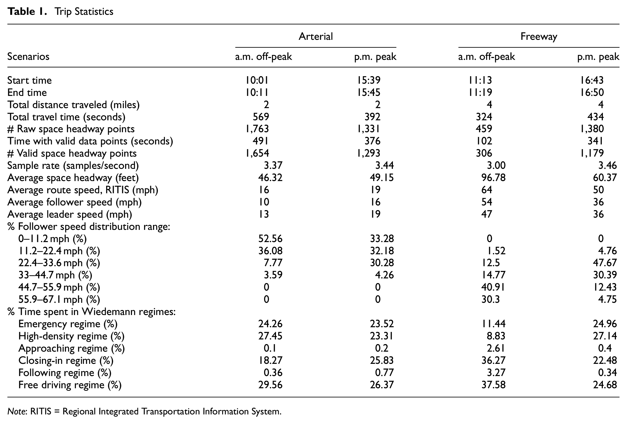
Note: RITIS = Regional Integrated Transportation Information System.

The average space headways in the arterial scenarios were around 46 to 49 ft. In the two arterial scenarios, the follower speed was less than the leader speed and the average speed in the segment as obtained from RITIS. The speed data distribution was varying, in the a.m. off-peak, around 88.64% of the speed observations were between 0 and 22.4 mph. Whereas in the p.m. peak, 65.46% of the speed observations were between 0 and 22.4 mph and 30.28% between 33.6 and 44.7 mph. The percentages of time spent across different regimes in the two arterial scenarios were similar. The data points were well spread across emergency, high density, closing-in, and the free driving regimes in both the scenarios.

While considering the freeway scenarios, the total distance traveled in the freeway segment was 4 mi. The number of samples collected in the a.m. off-peak scenario in the freeway was less, mainly because of a lack of vehicles at that time of the day; however, the sample rate were consistent. The average space headway distance on the freeway in the a.m. off-peak was around 97 ft as expected because of lack of traffic. During the p.m. peak, the average space headway reduced to 60 ft. The average follower speed and the average leader speed were less than the average speed across the segment (RITIS). In the a.m. off-peak scenario, 73.85% of the observations were in the closing-in and free driving regime and 71.21% of the speed observations were between 44.7 and 67.1 mph. In the p.m. peak scenario on the freeway, the regime distribution resembled the arterial roads. However, 78.06% of the speed observations were between 22.4 and 45.7 mph, much lower than the a.m. off-peak scenario. For a similar regime distribution corresponding to the arterial segment, the driver was at a higher speed range.

Also, a sensitivity analysis is performed to understand the variance in the data distribution in the emergency regime during the p.m. peak. From Equation 7, we get

β = BXadd + BXmult * RND 1 n

(17)

β and ABX are positively correlated. Table 2 shows the results of the sensitivity analysis.

Table 2.

Sensitivity Analysis

	Emergency regime (%)
β	Arterial (p.m. peak)	Freeway (p.m. peak)
2.3	21.81	20.19
2.4	22.43	22.56
2.5	23.52	24.96
2.6	24.83	27.23
2.7	25.52	28.41

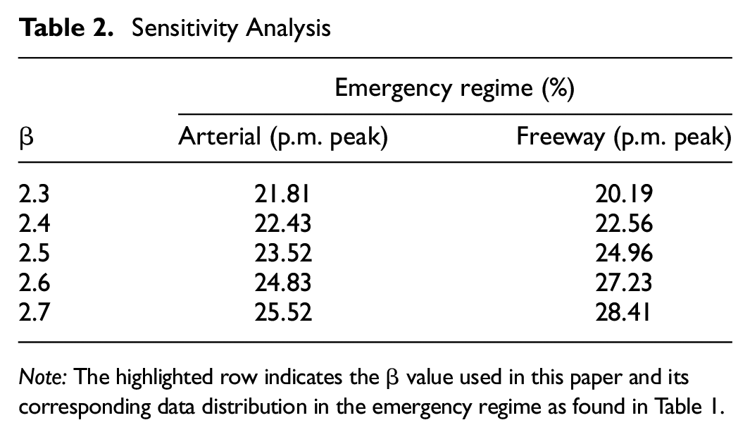
Note: The highlighted row indicates the β value used in this paper and its corresponding data distribution in the emergency regime as found in Table 1.

Based on the above analysis, there is a 3.71% variation in data distribution during the p.m. peak in the arterial segment and a variation of 8.22% during the p.m. peak in the freeway segment from the lowest assigned $β$ value. Therefore, it is understood that the variation in $β$ does not have a significant impact on the data distribution across the emergency regime, but the freeway data is slightly more sensitive to the $β$ parameter than the arterial data.

Longitudinal Evolution of Local Density

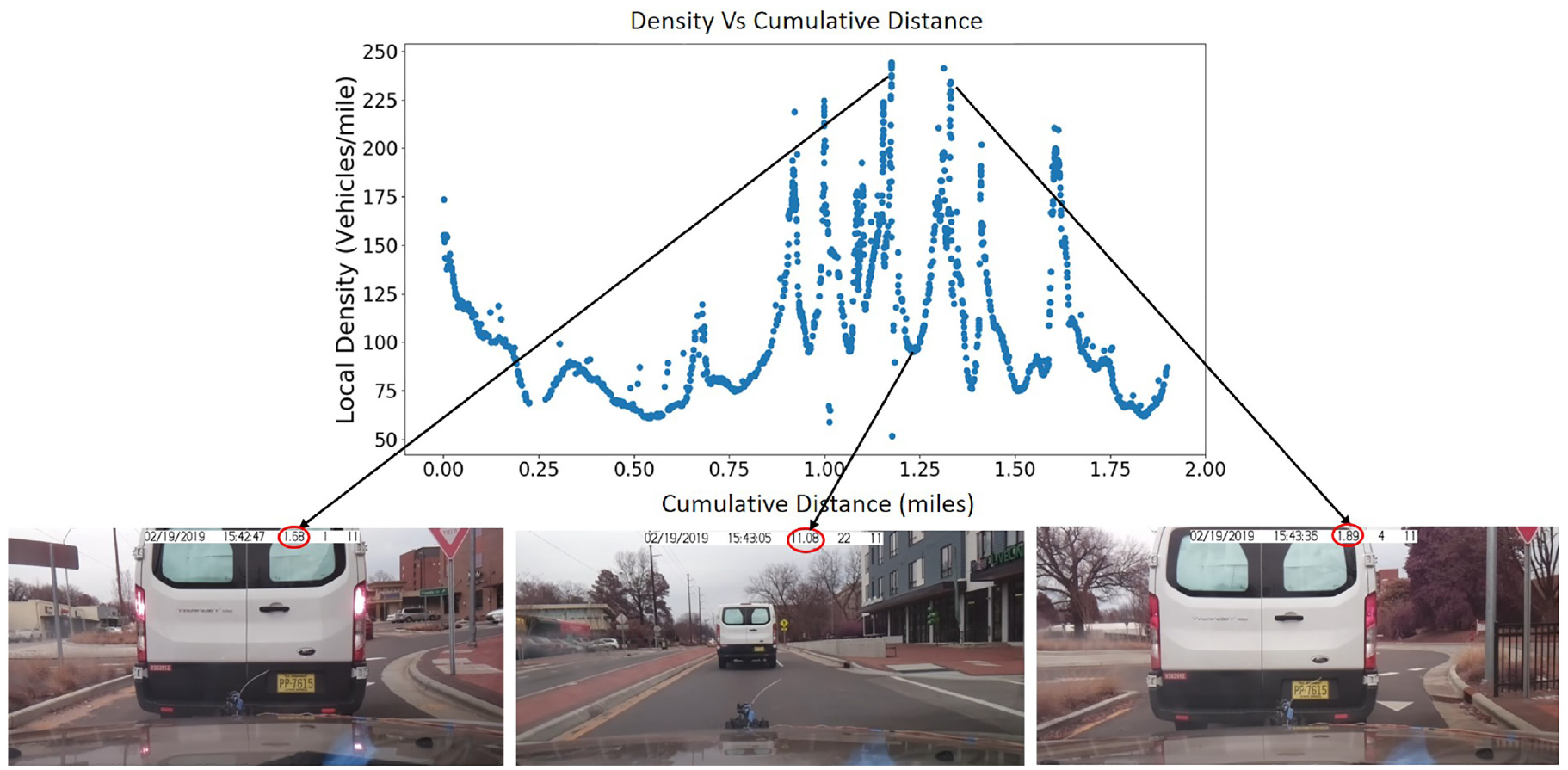
In this section, we visualize key aspects of the estimated local density through its scatter plot against the route path supplemented by photos captured in real-time.

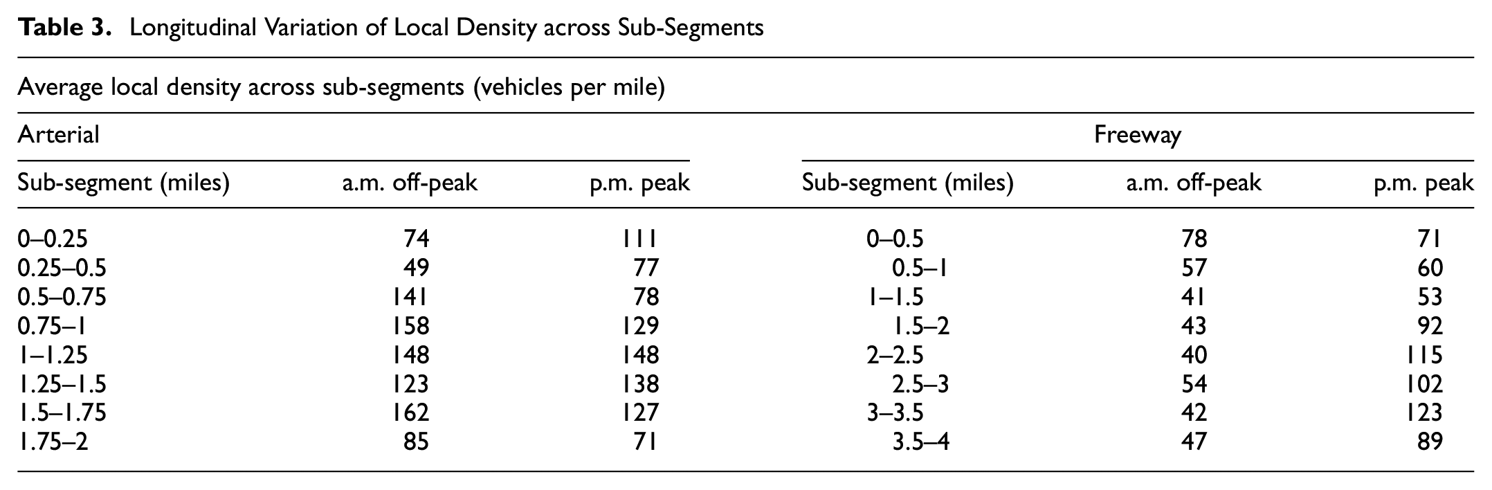
Figure 4 highlights the local density plot over cumulative distance for the arterial segment in the p.m. peak scenario. This plot helps in identifying the local density at precise locations across the corridor. Such plots of longitudinal evolution across a corridor provide a sense of constraints forced constraints on the driver by traffic stream and road geometry. For example, three spots on the plot are highlighted through actual images captured in real time. The first image indicates the high density at the entrance of a roundabout, as we expect vehicles to yield while the queue builds up at the entrance of the roundabout. In the second image, the leading vehicle creates a large headway as a result of exiting the roundabout, and correspondingly the density decreases. In the third image, similar to the first one, the leader yields at the entrance of another roundabout. As the queue builds up the density also increases. Table 3 summarizes the average local density for every 0.25 mi of the a.m. off-peak and p.m. peak data from the arterial segment and every 0.5 mi of the a.m. off-peak and p.m. peak data from the freeway segment.

Table 3.

Longitudinal Variation of Local Density across Sub-Segments

Average local density across sub-segments (vehicles per mile)
Arterial			Freeway
Sub-segment (miles)	a.m. off-peak	p.m. peak	Sub-segment (miles)	a.m. off-peak	p.m. peak
0–0.25	74	111	0–0.5	78	71
0.25–0.5	49	77	0.5–1	57	60
0.5–0.75	141	78	1–1.5	41	53
0.75–1	158	129	1.5–2	43	92
1–1.25	148	148	2–2.5	40	115
1.25–1.5	123	138	2.5–3	54	102
1.5–1.75	162	127	3–3.5	42	123
1.75–2	85	71	3.5–4	47	89

Figure 4.

Local density profile across the arterial segment in the p.m. peak.

Table 3 gives the average local density distribution across sub-segments of both freeway and arterial corridors. In the arterial section, there is a higher local density between the 0.5 and 0.75 mi segment in the a.m. off-peak than in the p.m. peak. If this trend continues among other drivers, then the reason for such density variations can be investigated through location inspection.

In the freeway corridor during the a.m. off-peak period, all sub-segments show a low local density. On the other hand, there is a drastic increase in local density during the peak period between sub-segments 2 to 3.5 mi. The root cause behind these high local densities of these sub-segments must be of interest to planners and regulatory officers if the same pattern recurs on multiple weekdays.

Relationship between Instantaneous Speed and Local Density by Microscopic Regimes

We have combined the two sets of arterial data (a.m. and p.m. data) and the two sets of freeway data (a.m. and p.m. data) and have analyzed them separately using a combination of microscopic and macroscopic models. In Figure 5, the pie charts represent the regime distribution for every 50 vehicles per mile (vpm) range. In Figure 5a the speeds ranged between 0 and 40 mph and in Figure 5b the speeds ranged between 15 and 65 mph. In both arterial and freeway segments, only four regimes (the free driving, closing-in, high density, and emergency) were predominant because the following regime and the approaching regime are more like a transition phase. Free driving and the closing-in are high-speed regimes where the free driving regime is achieved when the distance between the leader and the follower is increasing and the closing-in regime is achieved when the distance between the two is decreasing. The emergency regime and the high-density regimes are low-speed regimes, while the high-density driving regime is achieved when the distance between the leader and the follower is increasing and the emergency regime is achieved when the distance between the two is decreasing. A driver was considered a safe/neutral driver if the free driving regime was maintained at high speeds and high-density regime at low speeds.

Figure 5.

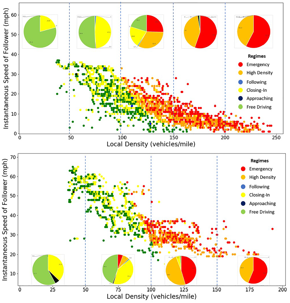
Combined instantaneous speed-local density relationship by Wiedemann regime for: (a) arterial; and (b) freeway.

In Figure 5, the arterial and the freeway plot displays a high percentage of the free-driving regime at a low local density of 0–50 vpm, that is, the driver maintains a safe distance at high speeds and low local densities. However, in both arterial and freeway segments, there is a high percentage of the emergency regime at high local densities (greater than 150 vpm and 100 vpm respectively) that is, the driver maintains very close distances at speeds higher than the leader, and chances of collision are higher. Therefore, from these analyses, the driver behavior can be characterized as a safe driver at low local densities and as an aggressive driver at high local densities. Driver behavior can, therefore, be characterized even with a local density of 35 vpm on freeways. (Figure 5)

Comparing Instantaneous Speed-Local Density with Macroscopic models

In this section, two simple yet popular macroscopic traffic stream models—Greenshields and modified Greenberg—are calibrated to the local density data for the freeway segments. Details of these two models can be found in this study ( 24 ).

The fitted parameters were estimated by minimizing the sum squared differences of the observed and modeled speed. Figure 6 shows the observed and fitted speed-density plot. Table 4 shows the fitted model parameters. Note that the data collected from the arterial segments were not included in this comparison since the models tested here were mostly applicable to uninterrupted traffic flow.

Table 4.

Fitted Traffic Model Parameters

Parameter	Fitted to Greenshields	Fitted to modified Greenberg
Free-flow speed (mph)	68	58
Jam Density (vpm)	206	200
Density at capacity (vpm)	103	74
Speed at capacity (mph)	34	48
Predicted capacity (vphpl)	3,502	3,552
Modified R-square (%)	72.20	73.30

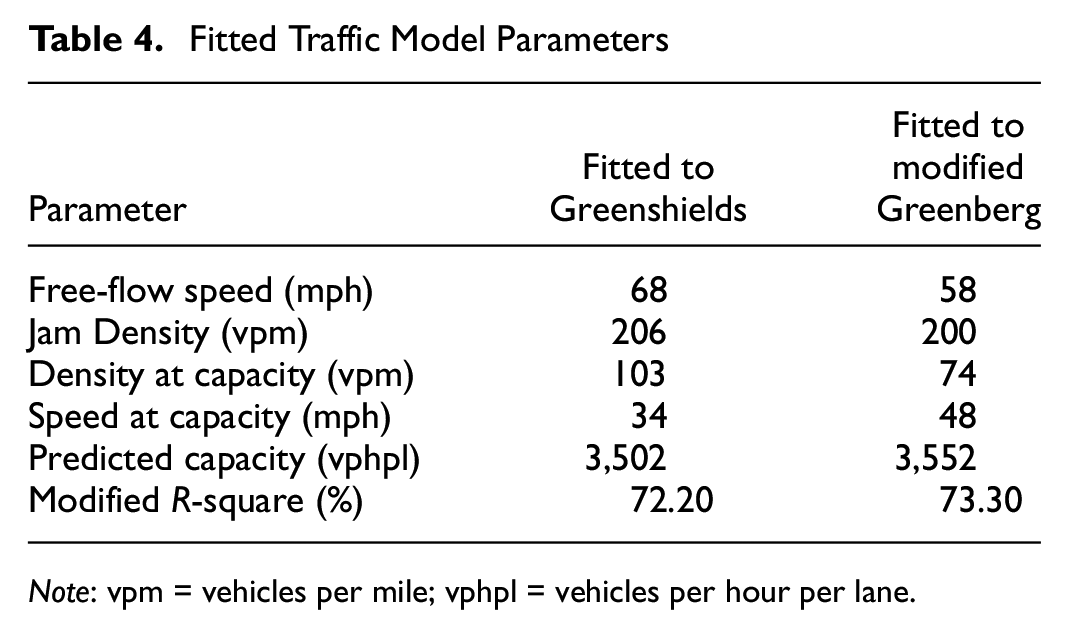
Note: vpm = vehicles per mile; vphpl = vehicles per hour per lane.

Figure 6.

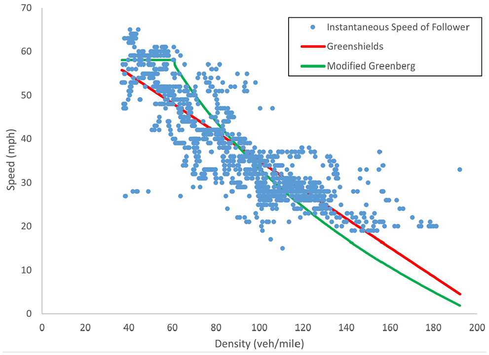
Instantaneous speed-local density data from the freeway segment versus macroscopic models.

Figure 6 and Table 4 show that both traffic stream models have a reasonable fit to the observed instantaneous speed and local density data as the Modified R-square values are greater than 70% for both models. The fitted jam density value matches very closely with the widely used 190 vpm ( 23 ). The fitted free-flow speed and speed at capacity values are within reasonable ranges given that the posted speed limit at the segments was 60 mph. However, the number of observations in a free-flow condition was low in this data set. This was because vehicles tend to maintain a large space headway when traveling at a high speed, while the lidar unit used in this research was limited to about 40 m.

The capacity and the resulting density at capacity are unusually high from the macroscopic traffic flow perspective. Conventional traffic flow theory suggests that the capacity of freeway segments does not exceed 2,400 vehicles per hour per lane (vphpl) ( 23 ), while the fitted capacity here is above 3,500 vphpl for both models. This discrepancy is attributed to the observed data representing a single individual’s naturalistic driving characteristics rather than the average traffic stream characteristics. For an individual driver, the expected capacity at freeway segments is 2,400 vphpl ( 23 ), but from the above analysis, the observed flow rate of the driver is 3,500 vphpl which interprets the driver to be driving with a headway of approximately 1 s. While it is unrealistic for all drivers in a traffic stream to keep such a short headway, an individual driver may certainly exhibit such an aggressive characteristic in some cases. These findings also underscore the importance of such a local-level speed-density analysis for evaluating both naturalistic driving and autonomous vehicle driving algorithms.

Conclusions

This paper developed methodologies to infer from local density collected using a custom-built system comprising a low-cost lidar sensor. The sensor data collected for this research consist of microscale observation from a single driver using a lidar and a GPS. The ubiquity of similar sensor-based data is expected with the wide deployment of connected and automated vehicles. The paper developed a methodology to model driving behavior by capturing the varying reactions of a single driver with changing local density along a corridor. The proposed framework can be applied to similar data collected for multiple drivers operating at the same time in a traffic stream. It can be used to investigate local interactions between heterogeneous vehicle classes such as human driver–human driver, human driver–automated vehicle, light-duty vehicle–heavy-duty vehicle, and so forth. Such a locally developed driving behavior model will be more pertinent in the near future because of the predicted pervasiveness of sensor-equipped vehicles and mixed operations of different vehicle types.

Focusing on the longitudinal car-following behavior, the data presented in this paper show that, for a lead vehicle within range, a lidar sensor can duplicate its trajectory over time. Also, insights into the local density at precise locations across the corridor were obtained, which explains the trend in driver behavior along a corridor. More importantly, local density as a function of speed can be formulated to describe the driver (or in the case of automation, AV software) behavior. The data were categorized into various Wiedemann car-following regimes and analyzed with Speed-Density graphs to understand driver behavior. It highlighted the differences in the regime allocations between facility types and congestion levels.

The speed and density data were fitted against the Greenshields and modified Greenberg models, which resulted in a Modified R-square value greater than 70% in both cases. The estimated driver-based capacity was found to be greater than 3,500 vph for both models where the conventional capacity according to the HCM-6 model is 2,400 vph ( 23 ), which clearly defines an overall aggressive driver behavior across the segment.

At present, the AV sensor observations are not widely available to agencies; however, in future there is a high likelihood of manufacturers opening the availability of such data to transportation agencies, insurance companies, or even directly to consumers. With similar data from vehicles traveling through the same corridor at the same time, it will be possible to evaluate traffic characteristics representing the entire corridor. In such a case, trajectory level local density data from multiple vehicles must be aggregated/stitched over time and space. Further research is needed in the area of lane-changing behavior, and in determining other safety criteria beyond Wiedemann regimes, such as time-to-collision (TTC) and safety margins. Such driving characteristics can be used to explore fuel consumption studies. Those will help in developing and modeling robust AV software to handle human driving exceptions when AVs will coexist with human drivers.

Footnotes

Acknowledgements

The authors of this paper would like to thank Thomas Chase, Rachana Gupta, Gyounghoon Chun, and Lokeshwar Deenadayalan for their valuable support throughout this project.

Author Contributions

The authors confirm contribution to the paper as follows: study conception and design: A. Azhagan, T. Shams, R. Nagui; data collection: A. Azhagan; analysis and interpretation of results: A. Azhagan, T. Shams, R. Nagui, A. Ishtiak; draft manuscript preparation: A. Azhagan, T. Shams, R. Nagui, A. Ishtiak. All authors reviewed the results and approved the final version of the manuscript.

Declaration of Conflicting Interests

The author(s) declared no potential conflicts of interest with respect to the research, authorship, and/or publication of this article.

Funding

The author(s) disclosed receipt of the following financial support for the research, authorship, and/or publication of this article: This research was funded partially by the U.S. Department of Energy (DOE) Advanced Research Project Agency-Energy (ARPA-E) through its TRANSNET Program and a project led by the National Transportation Center at the University of Maryland.

The findings presented in this paper do not necessarily represent the official views of Department of Energy (DOE) or ARPA-E. The authors are solely responsible for all statements in the paper.

References

Coifman

Freeway Detector Assessment: Aggregate Data from Remote Traffic Microwave Sensor. Transportation Research Record: Journal of the Transportation Research Board, Vol. 1917, 2005, pp. 149–163.

Lee

S.-H.

Lee

B.-W.

Yang

Y.-K.

Estimation of Link Speed Using Pattern Classification of GPS Probe Car Data. Computational Science and Its Applications – ICCSA, Vol. 3981, 2006, pp. 495–504.

Tanvir

Chase

R. T.

Roupahil

N. M.

Development and Analysis of Eco-Driving Metrics for Naturalistic Instrumented Vehicles. Journal of Intelligent Transportation Systems, Vol. 1, 2019, p. 14. https://doi.org/10.1080/15472450.2019.1615486.

Ahmed

Karr

Rouphail

N. M.

Chun

Tanvir

Characterizing Lane Changes via Digitized Infrastructure and Low-Cost GPS. Transportation Research Record: Journal of the Transportation Research Board 2019. 2673: 298–309.

Catapang

A. N.

Ramos

Obstacle detection using a 2D LIDAR system for an Autonomous Vehicle. In 6th IEEE International Conference on Control System, Computing and Engineering (ICCSCE), Penang, Malaysia, 25–27 November 2016. IEEE, New York.

Azhagan

Shams

Nagui

M. R.

Rachana

Capturing Vehicular Space Headway Using Low-Cost LIDAR and Processing through ARIMA Prediction Modeling. Electrical Engineering and Systems Science - Signal Processing, arXiv:1907.11648, 2019.

Ren

Large-Scale Outdoor SLAM Based on 2D Lidar. Electronics, Vol. 8, No. 6, 2019, p. 613.

Mallikarjuna

Phanindra

Ramachandra Rao

Traffic Data Collection under Mixed Traffic Conditions Using Video Image Processing. Transportation Engineering, Vol. 135, No. 4, 2009, pp. 174–182. https://doi.org/10.1061/(ASCE)0733-947X(2009)135:4(174).

Panos

Prevedouros. Performance and Challenges in Utilizing Non-Intrusive Sensors for Traffic Data Collection. Advances in Remote Sensing, Vol. 2, 2013, pp. 45–50.

10.

Hartmann

Middleton

Morris

Assessing Vehicle Detection Utilization Video Image Processing Technology. Publication FHWA/TX-97/1467-4. Texas Department of Transportation, Texas, 1996.

11.

Prevedouros

P. D.

Papandreou

Kopelias

Vegiri

Video Incident Detection Tests in Freeway Tunnels. Transportation Research Record: Journal of the Transportation Research Board, 2006. 1959: 130–139.

12.

Darema

Dynamic Data Driven Applications Systems: A New Paradigm for Application Simulations and Measurements. Computational Science – ICCS, Vol. 3038, 2004, pp. 662–669.

13.

Chen

S.-H.

Pan

J.-S.

Driving Behavior Analysis Based on Vehicle OBD Information and AdaBoost Algorithms. Lecture Notes in Engineering and Computer Science, Vol. 1, 2015, pp. 102–106.

14.

Reininger

Miller

Zhuang

Cappos

A First Look at Vehicle Data Collection via Smartphone Sensors. In IEEE Sensors Applications Symposium (SAS), Zadar, Croatia, 13–15 April 2015. IEEE, New York.

15.

de Fabritiis

Ragona

Valenti

Traffic Estimation and Prediction Based on Real Time Floating Car Data. In 11th International IEEE Conference on Intelligent Transportation Systems, Beijing, China, 12–15 October 2008. IEEE, New York.

16.

Wang

Dixon

K. K.

Hunter

Operating-Speed Model for Low-Speed Urban Tangent Streets Based on In-Vehicle Global Positioning System Data. Transportation Research Record: Journal of the Transportation Research Board, 2006. 1961: 24–33.

17.

Gurusinghe

G. S.

Nakatsuji

Azuta

Ranjitkar

Tanaboriboon

Multiple Car-Following Data with Real-Time Kinematic Global Positioning System. Transportation Research Record: Journal of the Transportation Research Board, 2002. 1802: 166–180.

18.

Neal

LIDAR vs RADAR. Published April 24, 2018. https://www.fierceelectronics.com/components/lidar-vs-radar. Accessed December 12, 2020.

19.

Janson

Tapani

O. A.

Comparison of Car-Following Models. Swedish National Road and Transport Research Institute, VTI Meddelande 960A, Linkoping, Sweden, 2004.

20.

Wiedemann

Reiter

Microscopic Traffic Simulation: The Simulation System MISSION, Background, and Actual State. Project ICARUS (V1052) Final Report, CORDIS European Commission, Brussels, Belgium, 1992.

21.

Higgs

Abbas

M. M.

Medina

Analysis of the Wiedemann Car Following Model over Different Speeds using Naturalistic Data. In 3rd International Conference on Road Safety and Simulation, Indiana, 2011. Transportation Research Board, Washington, D.C

22.

Regional Integrated Transportation Information System, https://ritis.org/intro. Accessed June 26, 2019.

23.

Transportation Research Board. Highway Capacity Manual Sixth Edition: A Guide for Multimodal Mobility Analysis, 6th ed. Transportation Research Board, Washington, D.C., 2016.

24.

Gerlough

D. L.

Huber

M. J.

. Traffic Flow Theory: A Monograph. Transportation Research Board, Washington, D.C., 1975.