Improving Interstate Freeway Travel Time Reliability Analysis by Clustering Travel Time Distributions

Abstract

Travel time reliability quantifies variability in travel times and has become a critical aspect for evaluating transportation network performance. The empirical travel time cumulative distribution function (CDF) has been used as a tool to preserve inherent information on the variability and distribution of travel times. With advances in data collection technology, probe vehicle data has been frequently used to measure highway system performance. One challenge with using CDFs when handling large amounts of probe vehicle data is deciding how many different CDFs are necessary to fully characterize experienced travel times. This paper explores statistical methods for clustering CDFs of travel times at segment level into an optimal number of homogeneous clusters that retain all relevant distributional information. Two clustering methods were tested, one based on classic hierarchical clustering and the other used model-based functional data clustering, to find out their performance on clustering distributions using travel time data from Interstate 64 in Virginia. Freeway segments and those within interchange areas were clustered separately. To find the proper data format as clustering input, both scaled and original travel times were considered. In addition, a non-data-driven method based on geometric features was included for comparison. The results showed that for freeway segments, clustering using travel times and the Anderson–Darling dissimilarity matrix and Ward’s linkage had the best performance. For interchange segments, model-based clustering provided the best clusters. By clustering segments into homogenous groups, the results of this study could improve the efficiency of further travel time reliability modeling.

Travel time reliability quantifies the variability in travel times and has become a critical aspect for evaluating transportation network performance. The Moving Ahead for Progress in the 21st Century Act (MAP-21) set one of the six national goals as “System reliability—improve the efficiency of the surface transportation systems.” Travel time reliability is defined as the consistency or dependability in travel times measured from day to day and/or across different times of the day according to the Federal Highway Administration (FHWA) ( 1 ). Travel time reliability can better quantify the benefits of traffic management and operations activities than average travel time. As a result, many transportation agencies have treated travel time reliability as a key measure for performance monitoring and evaluation, project prioritization, and resource allocation.

Currently, many state transportation agencies in the United States procure and use probe vehicle data frequently to measure highway system performance or for traveler information. This probe data provides wide coverage and also measures travel times on shorter segments, termed traffic message channel (TMC) segments. While the “largeness” of this data is desirable, there can be substantial challenges extracting useful information beyond simple statistical summaries like the mean and standard deviation from the enormous amount of data collected. For performance measures such as travel time reliability, these simple statistics are not enough. It is important to extract other relevant statistical information, such as the distribution of travel times that characterize the highway system. Historically, the empirical cumulative distribution function (CDF) has been used as a tool to preserve inherent information on the variability and distribution of travel times. Thus, the estimation of CDFs becomes a common prerequisite for travel time reliability prediction, which is quite a challenge when handling large amounts of probe vehicle data (e.g., data collected for an extended amount of time at a regional level). Fitting travel time data into single-mode or multi-state mixture mode distributions is a commonly used approach. A variety of distributions have been tested in previous studies, such as normal and lognormal ( 2 ), gamma and compound gamma ( 3 ), Weibull ( 4 ), Generalized Beta ( 5 ), Halphen distribution ( 6 ), and Burr distributions ( 7 ). The results from those studies often disagreed with each other because the underlying CDFs could be quite different, even for segments of the same corridor. Deciding how many different CDFs are necessary to fully characterize and predict experienced travel times is a significant challenge. Keeping and estimating separate CDFs for individual TMCs may not be practical or efficient from a data management and analysis perspective. On the other hand, using a single CDF for all TMCs poses the risk of substantial information loss, perhaps enough to render the CDF meaningless. One solution to this challenge is to first cluster TMCs with similar CDF shapes into the same group, then estimate CDFs at the group level to quantify impact factors and prediction, as shown in Figure 1. This study focused on the clustering step. CDF estimation will be discussed in a separate paper.

Figure 1.

Travel time reliability modeling process.

Specifically, this paper tested different statistical methods for clustering CDFs of travel times, observed on different TMCs, into an optimal number of homogeneous clusters that retain all relevant distributional information. Consolidating the information contained in hundreds or even thousands of different TMCs into a few homogeneous clusters can significantly enhance efficiency and facilitate the efforts by state Departments of Transportation (DOTs) aimed at: (i) understanding travel time reliability and its influencing factors; (ii) predicting reliability; and (iii) setting appropriate targets for the future.

Literature Review

The fundamental cause of travel time variability is the dynamic nature of the supply and demand components of the transportation system (e.g., traffic control devices and time-varying origin–destination volumes). Transient events such as incidents, work zones, inclement weather, and special events may also contribute to unreliable travel times. To know how to improve travel time reliability and what to expect from the investments and other influences over time, it is important to have a good understanding of all the factors that affect travel time reliability. Many previous studies have been conducted to explain how different factors affect reliability, including traffic incidents ( 8 – 11 ), inclement weather ( 12 – 14 ), work zones ( 15 , 16 ), and demand/capacity ( 8 , 17 ). One common issue with these previous studies is that, regardless of what mathematical methodologies were used, the conclusions of most studies were based on travel times at a corridor level, using long segments between loop detectors. In such cases, it is necessary to assume that factors considered in these studies had impacts on travel time reliability of the entire corridors or segments. This is not always an accurate reflection of the real situations since the studied corridors or segments were often fairly long. The travel time distributions at such an aggregated level are likely to be the results of impacts from multiple factors (and even unobserved ones), but most studies only attribute reliability impacts to whatever factors were under study. With advances in data collection technology, this study used probe vehicle data for which travel times are available at the much shorter TMC segment level. Travel time distributions could then be built and modeled more precisely at this level.

It is commonly seen from past studies that reliability analysis often starts with estimating travel time distributions, and the simplest way is fitting travel time data using single-mode probability distributions, as mentioned previously. Emam and Al-Deek ( 18 ) employed the Anderson–Darling (AD) goodness-of-fit statistics and the 90th percentile of absolute error to evaluate the performance of four different distribution types, namely Weibull, exponential, lognormal, and normal. The modeling results indicated that the lognormal distribution provided the best model fit. In addition, data from the same day of the week fit better than data collected across multiple weekdays because of the significant differences between traffic patterns across days. Li et al. ( 19 ) suggested that a lognormal distribution best characterized the distribution of travel times when a large time window (e.g., in excess of 1 h) was under consideration with the presence of congestion.

Little agreement could be found from previous studies about the right type of probability distribution. One essential reason behind this is the heterogeneity of the traffic system (e.g., background traffic, reliability impact factors, roadway geometric features). This is particularly true when travel time distributions are considered at the TMC segment level. It would be difficult to use a single distribution to represent travel times on all TMC segments, considering the various traffic conditions possible. However, it is also not practical to assign a unique distribution to every TMC segment. Clustering TMC segments into fairly homogeneous groups with similar travel time distributions, as an interim analysis step, can significantly reduce the number of possible travel time distributions under study, thereby making the modeling of travel time reliability and implementation easier and keeping the benefit of higher resolution probe vehicle data at the same time.

Clustering techniques have been used in classifying traffic patterns in previous studies. Weijermars and Van Berkum ( 20 ) applied Ward’s hierarchical clustering to cluster daily traffic flow profiles. To quantify the dissimilarity of daily flow profiles, several features, including the total daily flow, flow during peak hours, and the ratio of flow during peak and off-peak hours were used to characterize the daily flow profiles. They proposed a two-step clustering method. First, hierarchical clustering was applied to cluster flow profiles on each feature, resulting in a matrix with these features as columns and the cluster membership vector for each profile as rows. Then, hierarchical clustering was applied again using this matrix as input to obtain the final clusters. The authors also concluded that some pre-classification (e.g., classifying flow profiles to weekdays and non-weekdays) resulted in tighter clusters and suggested it as a way to improve cluster results. Similarly, both Azimi and Zhang ( 21 ) and Caceres et al. ( 22 ) adopted hierarchical clustering to group traffic flow profiles. However, they selected different features to characterize these profiles. Azimi and Zhang ( 21 ) used speed, while Caceres et al. ( 22 ) used roadway location defined by a factor, called the Relative Attractiveness Factor (RAF), calculated as a function of the distance to the nearby attractions.

Guardiola et al. ( 23 ) took the functional data analysis point of view to perform clustering of daily traffic profiles. They used the curves constructed by daily flows instead of other selected features for clustering. The curves were represented by the scores resulting from functional Principal Component Analysis (PCA). The clustering was then conducted using the Partitioning Around Medoids (PAM) algorithm, which is one of the most common realizations of k-medoid clustering ( 24 ).

In summary, clustering travel time distributions of TMC segments is considered a practical and efficient way to extract meaningful information from the large probe vehicle data that could improve travel time reliability analysis. A variety of clustering methods have been applied in the transportation field, as discussed above, but whether they are suitable for travel time distributions or how to adjust these methods for travel time distributions is seldom mentioned. For this study, two clustering methods were tested, one based on classic hierarchical clustering while the other used model-based functional data clustering, to find out their performance on clustering distributions.

Methods

The goal of clustering travel time distributions is to identify similarities among travel time distributions and group homogeneous TMCs into clusters, allowing TMCs within the same cluster to be represented by one distribution shape. In addition, as mentioned in the literature review, some pre-classification is suggested to improve the clustering result ( 20 ). For this study, the facility type (freeway segments or interchange) is assumed to play an important role in distinguishing distributions since traffic interacts more because of merging and diverging at interchanges, so this was selected as the pre-classification factor. Thus, data is divided into freeway and interchange groups before clustering.

The main question to answer before applying any clustering algorithm (e.g., k-means, hierarchical, or model-based) is how to measure the similarity between CDFs without knowing the exact functional expressions, which leads to the consideration of nonparametric methods of comparing distributions. Two nonparametric approaches are adopted in this paper, namely the Kolmogorov–Smirnov (KS) test and the Anderson–Darling (AD) test. They both quantify the differences between CDFs using defined statistical values (discussed later). Then, hierarchical clustering algorithms are applied based on these statistics.

Alternatively, travel times comprising CDF curves could be treated as functional data so that they can be approximated using dimension reduction techniques and represented by a set of finite parameters. Model-based clustering algorithms are then applied based on these parameters (discussed later). Both the nonparametric and model-based clustering methods mentioned above are considered to be data driven. To evaluate the benefit and necessity of data-driven approaches, clustering by the geometric features of TMC segments is also conducted for comparison. Figure 2 summarizes the methodologies used in this paper.

Figure 2.

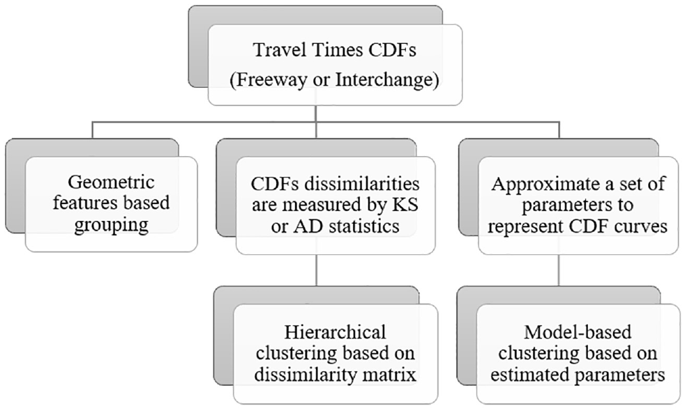
Methodology summary.

Geometric Features Clustering

Travel time distributions result from interactions among many factors, the geometric features of which have been identified and studied frequently in the past ( 11 , 18 , 25 ). The geometric factor included in this study is the number of through lanes. One primary advantage of this method is the convenience for practitioners because each cluster could be easily indexed using geometric feature(s). However, the underlying assumption that TMC segments with homogenous geometric characters will have similar shapes of travel time distributions could be biased and lead to inaccurate modeling results.

Nonparametric Distribution Clustering

Since there is no prior information about the mathematical representations of travel time CDFs, nonparametric methods are used to quantify the dissimilarity between distributions. The Kolmogorov–Smirnov (KS) test is commonly used for that purpose. For any two TMCs with CDFs $F_{n} (x)$ and $F_{m} (x)$ , the two-sample KS statistic is defined as D_n,m, which is the maximum distance between two distributions:

D_{n, m} = \sqrt{\frac{n m}{n + m}} s u p_{t \in ℝ} | \hat{F_{n} (x)} - \hat{F_{m} (x)} |

(1)

The distance reflects any difference resulting from the location and shape of two distributions, and any point change could have a significant impact on the value of the KS statistic. As mentioned earlier, the purpose of clustering analysis here is for modeling travel time reliability, which requires more focus on the tails of CDFs. In other words, we would like the resulting clusters to have the most similar shape at higher percentiles (e.g., above the 80th) within each group.

As an alternative option, the Anderson–Darling (AD) test, another nonparametric method, is also adopted for this study because it is particularly sensitive to the differences at the tails of distributions by assigning larger weights ( 26 ). The two-sample AD statistic is defined as:

A_{n m}^{2} = \frac{n m}{n + m} \sum_{- \infty}^{+ \infty} {[F_{n} (x) - F_{m} (x)]}^{2} ψ (H_{n + m} (x)) d H_{n + m} (x)

(2)

where $ψ (u) = \frac{1}{u (u - 1)}, 0 \leq u \leq 1$ is the weight function, and $H_{n + m} (x) = \frac{n}{n + m} F_{n} (x) + \frac{m}{n + m} F_{m} (x)$ is the empirical function of joint two samples.

The KS and AD statistics were calculated between each pair of TMC segments to form a dissimilarity matrix, with each row presenting the dissimilarity between one TMC and the rest.

An agglomerative hierarchical clustering method was then applied to rearrange rows in the KS and AD matrices so that similar ones could be paired together. The process starts with singleton clusters at the bottom level and continues to merge two clusters at a time to build a bottom-up hierarchy, called a dendrogram. There are several widely used methods to measure cluster distances, namely single linkage ( 27 ), complete linkage ( 28 ), group average ( 29 ), and Ward’s criterion ( 30 ). Single linkage takes the similarity between two clusters as the closest pair (nearest neighbor). Because of this behavior, a major drawback of this algorithm is that it is sensitive to noise and outliers. In contrast, complete linkage measures the similarity between two clusters as the furthest pairs (furthest neighbor). This will result in more compact clusters but sometimes assign observations to a group that is not the closest. As a compromise between these extreme situations, the group average uses the average distance, called the centroid, of every pair between two clusters. Since the members of clusters change at each step, computing centroids could be computationally expensive depending on the data size. Ward’s criterion determines the distance between two clusters using how much the merging cost will increase when they merge. After a thorough consideration of the advantages and disadvantages of the above methods, the complete linkage and Ward’s criterion methods were selected for further analysis. Some reasonable options of the number of clusters could be obtained from a dendrogram and tested along with options of AD/KS matrix and linkage options to get the preferred clustering results.

It is worth mentioning that since travel times used to construct CDFs are from TMCs with different lengths, the different scales of travel times might also contribute to dissimilarity, affecting the clustering results. As a result, scaled travel time data were clustered separately and then compared with the original travel time data clustering to decide whether scaled data were beneficial. Scaled travel time here refers to the difference between travel time and minimum value divided by the difference between maximum and minimum values, which only removes the unit of travel times but does not change the shape of a distribution.

The factors considered in nonparametric clustering and their levels are listed below, and the combination of them results in a total of 132 cases being tested:

Facility type: freeway, interchange

Data format: original, scaled (for KS statistics)

Input dissimilarity matrix: KS statistics, AD statistics

Linkage method: complete, Ward’s

Number of clusters evaluated: 10 to 20

The clustering performance resulting from each case was evaluated using the R package ‘clValid’ ( 31 ). This package offers a variety of measurements of cluster quality, including Dunn’s Index ( 32 ), silhouette width ( 33 ), connectivity ( 34 ), and stability ( 35 ). Dunn’s Index is the minimum distance between cluster points divided by the maximum cluster diameter. Higher values of Dunn’s Index indicate better separated and more compact clusters. The silhouette width is the weighted average of each observation’s silhouette value. The silhouette value measures the degree of confidence in a particular clustering assignment. It lies in the interval [−1,1], with well-clustered observations having values near one and poorly clustered observations having values near −1. The connectivity indicates to what degree the clusters are connected. This measure has a value between 0 and infinity and should be minimized. The stability measures are a special version of internal measures that evaluate the stability of a clustering result by comparing it with the clusters obtained by removing one column at a time. These measures include the average proportion of non-overlap (APN), the average distance (AD), the average distance between means (ADM), and the figure of merit (FOM). In all cases, the average is taken over all the deleted columns, and all measures should be minimized.

Model-Based Functional Data Clustering

As discussed above, the functional expressions of the CDF curves are unknown. As a result, the first step when clustering functional data is usually the reconstruction of the functional expressions using discrete observed data. This could be done by assuming that the CDF curves of $L_{2} [0, T]$ belong to a finite-dimensional space spanned by a basis of p-dimension functions $ψ_{1} (t), \dots, ψ_{p} (t)$ . Then, the CDF curve of the $i$ -th TMC, $f_{i}$ follows the expansion:

f_{i} (t) = \sum_{j = 1}^{p} γ_{ij} ψ_{j} (t)

(3)

where $ϒ = (γ_{i})$ is the matrix of expansion coefficients.

Bouveyron et al. ( 36 ) introduced an unobserved random variable, $Z = (Z_{1}, \dots, Z_{K}) \in {0, 1}^{k}$ , to indicate the cluster membership of $f_{i}$ , where $Z_{K} = 1$ means $f_{i}$ belongs to the k-th cluster, and otherwise when $Z_{K} = 0 .$ The clustering task is to obtain the value of variable $Z$ , which is solved by the discriminative functional mixture (DFM) model. The DFM model takes a common latent subspace $F [0, T]$ of $L_{2} [0, T]$ to be the most discriminative subspace for the K groups spanned by a basis of d-dimension functions $ϕ_{1} (t), \dots, ϕ_{d} (t)$ , where $d < K, d < p .$ $ϕ_{j} (t)$ is a linear combination of $ψ_{j} (t)$ by $ϕ_{j} (t) = \sum_{l = 1}^{p} u_{jl} ψ_{l}$ . The matrix $U = (u_{jl})$ is orthogonal with a dimension of $p \times d$ . The CDF curve of $i$ -th TMC, $f_{i}$ , could then be expressed as:

f_{i} (t) = \sum_{b = 1}^{d} λ_{ib} ϕ_{b} (t)

(4)

where the latent expansion coefficients matrix $Λ = (λ_{ib})$ is assumed following a multivariate Gaussian distribution, conditionally on $Z_{K} = 1$ :

Λ_{| Z_{k} = 1} ~ N (μ_{k}, Σ_{k})

(5)

where $μ_{k} and Σ_{k}$ are the mean and the covariance matrices of the k-th group. In addition, $Λ$ has the following relationship with $ϒ$ and $U$ :

ϒ = U Λ + ε

(6)

where $ε \in R^{p}$ is an independent, random noise term following a multivariate Gaussian density $ε ~ N (0, E)$ .

Combining the previous distribution assumptions, the marginal distribution of $ϒ$ follows a mixture of Gaussian distribution:

p (ϒ) = \sum_{k = 1}^{K} π_{k} \emptyset (ϒ; U μ_{k}, U^{t} Σ_{k} U + E)

(7)

where $π_{k} = P (Z_{K} = 1)$ is the prior probability of the k-th group.

The expectation-maximization (EM) algorithm is applied in maximizing the likelihood of $p (ϒ)$ to obtain the value of variable $Z$ using the R package ‘FunFEM’ ( 36 ). This package also provides three criteria to evaluate clustering performance, including the Akaike information criterion (AIC), Bayesian information criterion (BIC), and Integrated Completed Likelihood (ICL). Similar to hierarchical clustering, a range of selected numbers of clusters are compared. Clustering results with the smallest value of the above criteria are preferred.

Clustering Evaluation and Comparison

Evaluation measures of each clustering method introduced above are used to select the optimal clustering results for that method. Since they are specific to each clustering method, it is necessary to find an empirical way to compare clusters resulting from different approaches. For this study, the goal of clustering TMC segments is to find homogeneous clusters that can be represented by unique distributions to build models for reliability analysis. The dependent variable of the reliability model could be selected from various reliability measures. Level of Travel Time Reliability (LOTTR) is the required reliability measure reported periodically by FHWA rulemaking ( 37 ). It is calculated as the ratio of the 80th percentile to 50th percentile travel time of each reporting segment. To address this particular need, the performance of optimal clusters resulting from different methods is then further evaluated by how close the 80th percentiles within each cluster are, using silhouette width. This method is tailored to the application being examined in this study and is not necessarily suitable for other applications.

Data Description for Case Study

To test the proposed clustering methods, Interstate 64 (I-64) in Virginia was selected to conduct a case study. Speed data of I-64 from December 2017 to November 2018 on weekdays (excluding both weekends and holidays) during the morning peak (6:00–10:00 a.m.) and evening peak (16:00–20:00 p.m.) periods were downloaded from the third-party probe data (INRIX) at hourly intervals, which were then converted into travel times. There were 2,407 h (about 0.31%) of missing data points across all TMCs. Since this was a small portion of overall data, they were removed from the data set. Segments of I-64 were classified into freeway and interchange groups based on the TMC labels, denoted as internal links (labeled with “P” or “N”) and external links (labeled with “+” or “−”), respectively. Internal segments represent a stretch of road within an interchange (e.g., between an exit ramp and an entrance ramp), defined as interchange segments. External segments represent a stretch of road between interchanges, referred to as freeway segments. Segments less than 0.1 mi long were removed to ensure the quality of data, resulting in a total of 375 TMC segments for both directions. The geometric data, the number of through lanes, was provided by the Virginia Department of Transportation and matched to the TMC segments based on spatial information. A statistical summary of travel times is illustrated in Table 1.

Table 1.

Statistical Summary of Data on I-64

Variable	Measure	Freeway (external)	Interchange (internal)
Number of TMC	Count	200	205
Length (miles)	Minimum	0.10	0.15
	Maximum	7.48	1.73
	Average	2.33	0.54
Travel times (seconds)	Minimum	5.56	7.88
	Maximum	5,828.64	1,284.72
	Average	138.53	33.48
Number of through lanes	Minimum	2	2
	Maximum	5	5

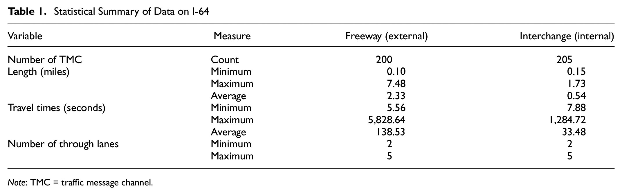
Note: TMC = traffic message channel.

Results Analysis

Clustering Results

Nonparametric Distribution Clustering

The first clustering method applied is hierarchical clustering based on the KS and AD statistics. As discussed in the methodology section, all TMCs were paired to measure their CDF dissimilarity using the KS and AD statistics, resulting in two pairwise dissimilarity matrices. These two matrices then became the input for hierarchical clustering. The results of hierarchical clustering could be visualized using a dendrogram. An example using the KS statistic and complete linkage with 10 clusters highlighted in different colors is shown in Figure 3. The differences between the heights of each level of branches indicate the distances between them. Figure 3 also shows that some CDFs are so different that they join a cluster alone or with few other TMCs at a higher height. These cases could be deemed to be outliers. To distinguish such CDFs, it is desirable to cut the tree before they merge into a bigger cluster. On the other hand, from a practical point of view, the resulting number of clusters should be manageable for practitioners to use. With these considerations in mind, a range of the optimal number of clusters from 10 to 20 was examined.

Figure 3.

Hierarchical clustering dendrogram (freeway, complete linkage).

Although dendrograms provide some useful insights into the optimal number of clusters, quantifying clustering performance is necessary to decide the exact preferred number of clusters and the best linkage method. The R package ‘clValid’ is able not only to calculate different performance measures including Dunn’s Index, silhouette width, connectivity, and stability (APN, AD, ADM, FOM) using different numbers of clusters but also to summarize the best results under each measure. Table 2 shows the KS based hierarchical clustering results using the “complete” linkage method and cluster numbers from 10 to 20 for freeway segments using the unscaled travel times. Each column represents the values of one performance measure for cluster sizes 10 to 20. The optimal size in the last row shows the clustering size that had the best performance under that particular measure. A silhouette width close to 1 is preferred, which in this case is the cluster size of 20. A higher value of Dunn’s Index is also preferred, which is the cluster size of 18. For the rest of the measures in Table 2, the minimum value indicates the best performance. The clustering size selected by most measures will be the optimal size. Table 2 shows a cluster size of 20 out-performs other options in four (silhouette, AD, ADM, and FOM) out of seven measures, thus becoming the preferred clustering size in this case. The same process was repeated for all 132 cases of different combinations of linkage methods, statistic matrix, facility types, data format, and cluster sizes. A summary of optimal clustering numbers is illustrated in Table 3.

Table 2.

Performance Measures for Cluster Size Selection (KS, “Complete” Linkage, Original Travel Times, Freeway Segments)

Cluster Size	Silhouette	Dunn	Connectivity	APN	AD	ADM	FOM
10	0.231	0.278	52.6528	0.054	1.912	0.122	0.113
11	0.236	0.285	57.906	0.046	1.832	0.106	0.109
12	0.256	0.287	62.901	0.043	1.757	0.134	0.106
13	0.246	0.237	72.850	0.039	1.712	0.097	0.104
14	0.258	0.238	73.643	0.033	1.655	0.112	0.102
15	0.264	0.238	79.014	0.042	1.623	0.132	0.101
16	0.280	0.253	82.112	0.015	1.538	0.041	0.093
17	0.295	0.255	85.477	0.016	1.485	0.047	0.092
18	0.300	0.258	86.691	0.017	1.446	0.050	0.091
19	0.314	0.260	90.580	0.020	1.393	0.056	0.088
20	0.324	0.265	94.313	0.014	1.341	0.039	0.083
Optimal size	20	12	20	20	20	20	20

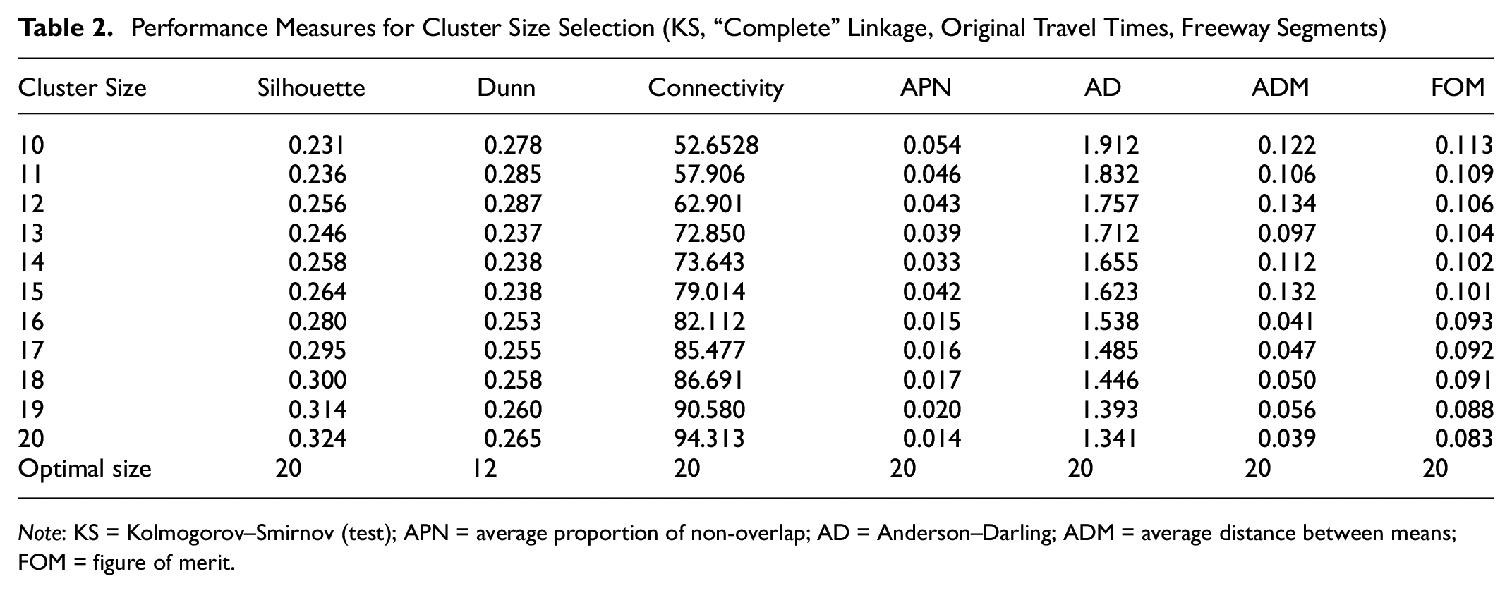
Note: KS = Kolmogorov–Smirnov (test); APN = average proportion of non-overlap; AD = Anderson–Darling; ADM = average distance between means; FOM = figure of merit.

Table 3.

Summary of Preferred Size of Clusters

Measure	Travel time					Scaled travel time
Linkage method	KS-ward’s	KS-complete	AD-ward’s	AD-complete	Model-based	KS-ward’s	KS-complete
Optimal cluster size: freeway	20	10	10	10	8	10	18
Optimal cluster size: interchange	15	20	10	20	4	20	10

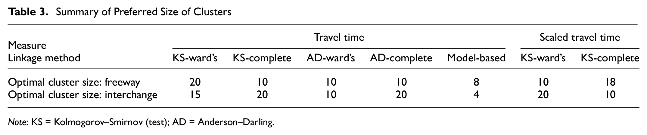
Note: KS = Kolmogorov–Smirnov (test); AD = Anderson–Darling.

Model-Based Functional Data Clustering

As described in the methodology, the first step for model-based functional clustering was to approximate the CDF curves using a basis of functions. Two decisions needed to be made during this step: selecting the type and the number of basis functions. There are different types of basis functions to choose from, including polynomials, spline, Fourier, wavelet, and so forth. The basis function should be selected according to the nature of the particular functional data. In general, a Fourier basis is suitable for periodical data, while a spline basis is the most common choice for non-periodic data ( 38 ). In this study, the latter is chosen because the interest is not travel times in a time series but rather the cumulative distribution during a specific period.

On visually analyzing the distribution curves, the curves are fairly flat until around the 85th percentile, where they change rapidly. As a result, it was decided to assign knots every 5% before the 80th percentile and every 1% after the 80th percentile to reflect the tails’ rapid change. For practical usability reasons mentioned previously, the maximum number of clusters was set as 20. Since there was no other information available, a range of clusters from 2 to 20 was considered for optimal cluster size selection.

Bouveyron et al. ( 36 ) advised that although AIC and BIC are commonly used metrics, they might be less effective for practical use. On the contrary, ICL can choose the number of clusters in a more separated manner and was thus selected to evaluate cluster performance for this study. As mentioned in the methodology, this model-based clustering algorithm uses a DFM model, and there are 12 types of submodels based on different covariance matrices. Under the “model” argument in “FunFEM,” it is possible to set the value as “all” to consider all submodels. Then, the R package calculates the ICL value for each cluster size under every submodel type. By the end of the run, the values of ICL under different submodels and cluster sizes will be summarized and ranked automatically. After comparing ICL for cluster sizes from 2 to 20 under each submodel type, a cluster size of 8 was preferred for freeway segments and 4 for interchange segments, as summarized in Table 3.

Clustering Interpretation and Comparison

Traditionally, roadway segments are grouped by their geometric features. One primary advantage of this method is the convenience of building models and interpreting the results. However, the underlying assumption that segments with homogenous geometric characteristics have similar shapes of travel time distributions could be biased. It is useful to compare this grouping method with the two data-driven methods to further demonstrate the purpose of clustering. The geometric factor included in this study is the number of through lanes. Based on this factor, both the freeway and interchange segments were divided into four subgroups, as shown in Figure 4. The average silhouette width of the 80th percentiles of travel times in each cluster was used to measure the performance of different clustering methods. The average silhouette value for freeway and interchange clustering by geometric feature was −0.21 and −0.29, respectively, which indicates this was not a preferable clustering method.

Figure 4.

Clusters by geometric features.

The average silhouette results of hierarchical clustering and model-based clustering using their preferred sizes of clusters from Table 3 are summarized in Table 4. For freeway segments, original travel times using the AD dissimilarity matrix and Ward’s linkage had the best performance, and the optimal cluster size was 10 (Figure 5a). For interchange segments, the model-based clustering provided the best clusters, and the optimal cluster size was 4 (Figure 6a). The travel time distribution of freeway segments overall had a less curved shape than distributions of interchange segments. The model-based functional data clustering could offer better results since this type of clustering’s typical applications are often curves with peaks or time-series data. It could also be concluded that scaled data did not help obtain better clustering results. So, for the data in this study, the original travel time data should be used to ensure both scale and location differences are captured. Also, most results using the AD matrix were better than using the KS matrix. Since the silhouette value of the 80th percentiles was used to evaluate the clustering results, this demonstrated that the AD test is better suited to travel time reliability analysis since the focus is on distribution tails.

Table 4.

Average Silhouette Width of the 80th Percentiles of Travel Time

Clustering approach	Linkage method	Average silhouette
		Freeway segment	Interchange segment
Hierarchical, travel time: KS	Ward’s	0.19	0.19
	Complete	0.17	0.11
Hierarchical, scaled travel time: KS	Ward’s	−0.30	−0.31
	Complete	−0.52	−0.34
Hierarchical, travel time: Anderson–Darling	Ward’s	0.32	0.23
	Complete	0.09	0.02
Model-based	n/a	0.15	0.41
Geometric feature	n/a	−0.21	−0.29

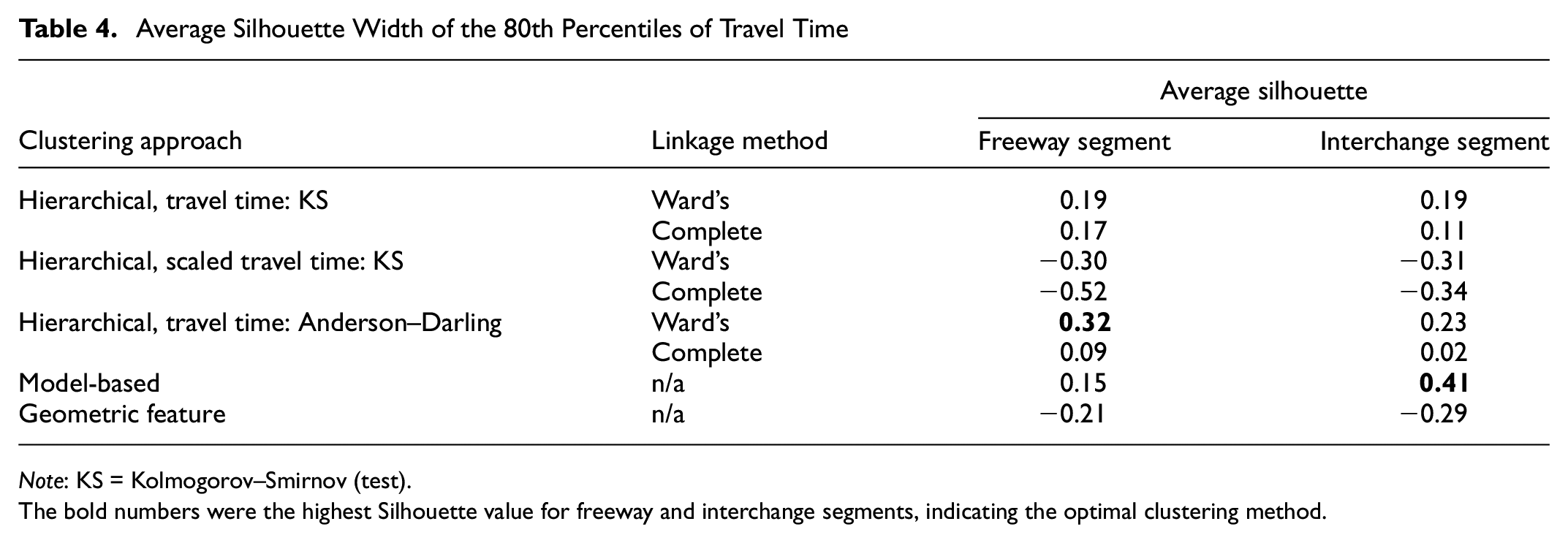
Note: KS = Kolmogorov–Smirnov (test).

The bold numbers were the highest Silhouette value for freeway and interchange segments, indicating the optimal clustering method.

Figure 5.

Final clustering result for freeway segments: (a) freeway CDF by clusters; and (b) reliability summary by freeway clusters.

Figure 6.

Final clustering result for interchange segments: (a) interchange CDF by clusters; and (b) reliability summary by interchange clusters.

In the final clustering results of freeway and interchange segments, Figures 5a and 6a show that each cluster has a unique overall distribution shape, especially in the tails. Distributions with shorter tails indicate that travel times from those clusters are more reliable than distributions with longer tails. To better quantify the reliability trend, Figures 5b and 6b summarize the average and standard deviation of the 80th percentile travel times and the LOTTR of each cluster. By clustering based on distribution shapes, it also clustered the segments to different reliability patterns, which could potentially be indicative of similar reliability impact factor(s). Previous studies indicate that certain travel time reliability measures are more sensitive to particular reliability impact factors. Most reliability measures rely on the travel time distributions, which relate different impact factors resulting in different distribution shapes. Further analysis will be conducted on that question.

Figure 7 plots the final clustering results of freeway segments geographically and demonstrates reliability patterns by location. Most segments along rural areas fell into clusters with relatively reliable travel times, while segments along urban areas were likely to be in clusters with lower reliability levels.

Figure 7.

Final freeway clusters locations.

Conclusions

This paper introduced the concept of clustering travel time distributions at the segment level into groups with homogenous shapes. Both data-driven, hierarchical, and model-based clustering and non-data driven, geometric feature clustering were applied, and the results were compared. The results showed that data-driven clustering methods produced high-quality clusters, with hierarchical clustering using an AD dissimilarity matrix and model-based clustering having better results than other combinations. This needs to be further tested using travel time data for a more extended period and more sites. The process of clustering serves as an interim step of the reliability analysis. It reduced the number of distributions from hundreds of unique values for individual segments to a limited number of distinct ones. As a result, instead of developing future prediction models for hundreds of individual segments, models are only necessary for each cluster.

Since most reliability measures are derived from travel time distributions, clustering based on distribution shapes also clusters reliability patterns resulting from different impact factors. According to SHRP 2 L03 ( 39 ), the sensitivity of reliability measures could change depending on the context of the application. For example, that report suggested that the 95th percentile is more sensitive to weather, and the 90th percentile is more sensitive to incidents. It is likely that different combinations of impact factors contribute to the heterogeneity of travel time distributions. As a result, by clustering travel time distributions into homogenous groups, it may help separate segments experiencing generally similar impact factor(s) into the same group, which could potentially improve the explanatory ability of the resulting reliability models. This is only our hypothesis based on the current study; to identify and quantify the exact impact factors for each cluster, the next step after clustering is to apply proper modeling techniques. For example, since most reliability measures rely on the travel time distributions, especially upper tails such as the 80th, 90th, or 95th percentile, quantile regression could be applied to identify significant impact factors for each cluster and predict reliability.

Footnotes

Author Contributions

The authors confirm contribution to the paper as follows: study conception and design: Xiaoxiao Zhang, Mo Zhao, Justice Appiah, Michael D. Fontaine; data collection: Xiaoxiao Zhang, Mo Zhao, Justice Appiah; analysis and interpretation of results: Xiaoxiao Zhang, Mo Zhao, Justice Appiah, Michael D. Fontaine; draft manuscript preparation: Xiaoxiao Zhang, Mo Zhao, Justice Appiah, Michael D. Fontaine. All authors reviewed the results and approved the final version of the manuscript.

Declaration of Conflicting Interests

The author(s) declared no potential conflicts of interest with respect to the research, authorship, and/or publication of this article.

Funding

The author(s) disclosed receipt of the following financial support for the research, authorship, and/or publication of this article: This paper was based on research funded by the Virginia Department of Transportation, project Investigation of the Factors that Affect Travel Time Reliability (grant number: 114313).

References

Federal Highway Administration. Travel Time Reliability. U. S. Department of Transportation, Washington, D.C., 2005.

Analytic Relationships between Travel Time Reliability Measures. Transportation Research Record: Journal of the Transportation Research Board, 2011. 2254: 122–130.

Kim

Mahmassani

H. S.

Compound Gamma Representation for Modeling Travel Time Variability in a Traffic Network. Transportation Research Part B: Methodological, Vol. 80, 2015, pp. 40–63.

Arroyo

Kornhauser

A. L.

Modeling Travel Time Distributions on a Road Network. Presented at 84th Annual Meeting of the Transportation Research Board, Washington, D.C., 2005.

Castillo

Nogal

Menéndez

J. M.

Sanchez-Cambronero

Jimenez

Stochastic Demand Dynamic Traffic Models Using Generalized Beta-Gaussian Bayesian Networks. IEEE Transactions on Intelligent Transportation Systems, Vol. 13, No. 2, 2011, pp. 565–581.

Delhome

Billot

El Faouzi

N. E.

Travel Time Statistical Modeling with the Halphen Distribution Family. Journal of Intelligent Transportation Systems, Vol. 21, No. 6, 2017, pp. 452–464.

Taylor

M. A.

Fosgerau’s Travel Time Reliability Ratio and the Burr Distribution. Transportation Research Part B: Methodological, Vol. 97, 2017, pp. 50–63.

Lint

H. van

Zuylen

H. van

. The Effects of Traffic Accidents on Travel Time Reliability. Proc., 2008 11th International IEEE Conference on Intelligent Transportation Systems, Beijing, China, October 12, 2008, pp. 79–84. IEEE.

Wright

Zou

Wang

Impact of Traffic Incidents on Reliability of Freeway Travel Times. Transportation Research Record: Journal of the Transportation Research Board, 2015. 2484: 90–98.

10.

Hojati

A. T.

Ferreira

Washington

Charles

Shobeirinejad

Reprint of: Modelling the Impact of Traffic Incidents on Travel Time Reliability. Transportation Research Part C: Emerging Technologies, Vol. 70, 2016, pp. 86–97.

11.

Charlotte

Sandra

Empirical Estimation of the Variability of Travel Time. Transportation Research Procedia, Vol. 25, 2017, pp. 2769–2783.

12.

Yazici

M. A.

Kamga

Singhal

Weather’s Impact on Travel Time and Travel Time Variability in New York City. Transportation Research, Vol. 40, 2013, p. 41.

13.

Caceres

Hwang

Estimating Freeway Route Travel Time Distributions with Consideration To Time-of-Day, Inclement Weather, and Traffic Incidents. Journal of Advanced Transportation, Vol. 50, No. 6, 2016, pp. 967–987.

14.

Zhang

Chen

Quantifying the Impact of Weather Events on Travel Time and Reliability. Journal of Advanced Transportation, Vol. 2019, 2019, pp. 1–9.

15.

Edwards

M. B.

Fontaine

M. D.

Investigation of Travel Time Reliability in Work Zones with Private-Sector Data. Transportation Research Record: Journal of the Transportation Research Board, 2012. 2272: 9–18.

16.

Srivastava

Chitturi

M. V.

Ahn

Rafferty

Analytical Methods for Work Zone Travel Time Reliability. InTrans Project 06-277. Smart Work Zone Deployment Initiative, Washington, D.C., 2018.

17.

Dowling

R. G.

Skabardonis

Margiotta

R. A.

Hallenbeck

M. E.

Reliability Breakpoints on Freeways. Presented at 88th Annual Meeting of the Transportation Research Board, Washington, D.C., 2009.

18.

Emam

E. B.

Al-Deek

Using Real-Life Dual-Loop Detector Data to Develop New Methodology for Estimating Freeway Travel Time Reliability. Transportation Research Record: Journal of the Transportation Research Board, 2006. 1959: 140–150.

19.

Rose

Sarvi

Using Automatic Vehicle Identification Data to Gain Insight Into Travel Time Variability and Its Causes. Transportation Research Record: Journal of the Transportation Research Board, 2006. 1945: 24–32.

20.

Weijermars

Berkum

Van E.

. Analyzing Highway Flow Patterns Using Cluster Analysis. Proceedings 2005 IEEE Intelligent Transportation Systems, Vienna, Austria, September 16, 2005, pp. 308–313. IEEE.

21.

Azimi

Zhang

Categorizing Freeway Flow Conditions by Using Clustering Methods. Transportation Research Record: Journal of the Transportation Research Board, 2010. 2173: 105–114.

22.

Caceres

Romero

L. M.

Benitez

F. G.

Estimating Traffic Flow Profiles According to a Relative Attractiveness Factor. Procedia-Social and Behavioral Sciences, Vol. 54, 2012, pp. 1115–1124.

23.

Guardiola

I. G.

Leon

Mallor

A Functional Approach to Monitor and Recognize Patterns of Daily Traffic Profiles. Transportation Research Part B: Methodological, Vol. 65, 2014, pp. 119–136.

24.

Kaufman

Rousseeuw

P. J.

Finding Groups in Data: An Introduction to Cluster Analysis. John Wiley & Sons, New York, NY, 2009.

25.

Bhouri

Aron

Scemama

Travel Time Reliability With and Without The Dynamic Use of Hard Shoulder: Field Assessment from a French Motorway. Journal of Traffic and Transportation Engineering (English Edition), Vol. 3, No. 6, 2016, pp. 520–530.

26.

Thas

Comparing Distributions. Springer, New York, NY, 2010.

27.

McQuitty

L. L.

Capabilities and Improvements of Linkage Analysis as a Clustering Method. Educational and Psychological Measurement, Vol. 24, No. 3, 1964, pp. 441–456.

28.

King

Step-Wise Clustering Procedures. Journal of the American Statistical Association, Vol. 62, No. 317, 1967, pp. 86–101.

29.

Sokal

R. R.

Numerical Taxonomy. Scientific American, Vol. 215, No. 6, 1966, pp. 106–117.

30.

Ward

J. H.

Jr.

Hierarchical Grouping to Optimize an Objective Function. Journal of the American Statistical Association, Vol. 58, No. 301, 1963, pp. 236–244.

31.

Brock

Pihur

Datta

clValid, An R Package for Cluster Validation. Journal of Statistical Software, Vol. 25, No. 4, 2008, pp. 1–22.

32.

Dunn

J. C.

A Fuzzy Relative of the ISODATA Process and Its Use in Detecting Compact Well-Separated Clusters. Journal of Cybernetics, Vol. 3, No. 3, 1973, pp. 32–57.

33.

Rousseeuw

P. J.

Silhouettes: A Graphical Aid to the Interpretation and Validation of Cluster Analysis. Journal of Computational and Applied Mathematics, Vol. 20, 1987, pp. 53–65.

34.

Handl

Knowles

Kell

D. B.

Computational Cluster Validation in Post-Genomic Data Analysis. Bioinformatics, Vol. 21, No. 15, 2005, pp. 3201–3212.

35.

Datta

Comparisons and Validation of Statistical Clustering Techniques for Microarray Gene Expression Data. Bioinformatics, Vol. 19, No. 4, 2003, pp. 459–466.

36.

Bouveyron

Côme

Jacques

The Discriminative Functional Mixture Model for a Comparative Analysis of Bike Sharing Systems. The Annals of Applied Statistics, Vol. 9, No. 4, 2015, pp. 1726–1760.

37.

Federal Highway Administration. National Performance Management Measures; Assessing Performance of the National Highway System, Freight Movement on the Interstate System, and Congestion Mitigation and Air Quality Improvement Program [Internet]. Vol. 82, Federal Register. 2017. pp. 5970–6050. https://www.federalregister.gov/d/2017-00681

38.

Ramsay

J. O.

Silverman

B. W.

Functional Data Analysis, 2nd ed. Springer, New York, NY, 2005.

39.

Cambridge Systematics and National Research Council. Analytical Procedures for Determining the Impacts of Reliability Mitigation Strategies. Transportation Research Board, Washington, D.C., 2013.