Enhancing the Accuracy of Peak Hourly Demand in Bike-Sharing Systems using a Graph Convolutional Network with Public Transit Usage Data

Abstract

With the growth of the bike-sharing system, the problem of demand forecasting has become important to the bike-sharing system. This study aims to develop a novel prediction model that enhances the accuracy of the peak hourly demand. A spatiotemporal graph convolutional network (STGCN) is constructed to consider both the spatial and temporal features. One of the model’s essential steps is determining the main component of the adjacency matrix and the node feature matrix. To achieve this, 131 days of data from the bike-sharing system in Seoul are used and experiments conducted on the models with various adjacency matrices and node feature matrices, including public transit usage. The results indicate that the STGCN models reflecting the previous demand pattern to the adjacency matrix show outstanding performance in predicting demand compared with the other models. The results also show that the model that includes bus boarding and alighting records is more accurate than the model that contains subway records, inferring that buses have a greater connection to bike-sharing than the subway. The proposed STGCN with public transit data contributes to the alleviation of unmet demand by enhancing the accuracy in predicting peak demand.

There has been a constant interest and steady growth in bike-sharing systems worldwide, led by expanding concerns about global motorization and climate change ( 1 ). People are becoming more active in protecting the environment, resulting in the increased use of eco-friendly modes such as public transportation and bike-sharing services. Bike-sharing services not only provide benefits from reduced traffic congestion and air pollution but also solve the first/last mile problem. Along with the start of the sharing economy, bike-sharing services have gained immense popularity worldwide for their convenience, time flexibility in usage, and the ability to acquire a bike at one location and return it to a different location.

However, like two sides of a coin, there are issues that the service operators must solve. As users can return their bikes anywhere, the number of bikes at a given station fluctuates from zero to a higher number than the station capacity. Given these circumstances, the systems sometimes fail because they cannot satisfy all demands from the users. Periodically, the bikes must be redistributed manually by truck drivers. To determine the number of bikes to be delivered and when and where to deliver them, it is necessary to predict the accurate demand at each station to apply effective rebalancing strategies. Prediction accuracy can be a significant factor in properly repositioning the bikes to maintain each station’s desired inventory level. That is because poor prediction may cause a spatial and temporal imbalance in bike stocks, which is essential from the perspective of potential users who want to rent out bikes ( 2 – 6 ). Studies need to be conducted to predict demands and minimize unmet demand so that users can be confident that the system works when they have a need.

To date, various methods have been used to predict the demand for a public bike-sharing system. Statistical models have been used to determine and quantify influential factors to the bike-sharing demand ( 7 – 11 ). Not only spatial and temporal properties but also weather or other exogenous variables have been found to be significant. As the neural network model has drawn significant attention, recent studies have tried to apply neural networks to predict demands ( 12 – 15 ). However, the problem with such models is their low accuracy around peak time. As more customers are restricted from using bike-sharing if the system fails in peak hours, it is crucial to predict the demand in peak hours accurately. Bike-sharing service is more likely to support transit services, and bike-sharing and transit systems have complex interactions that could support an operation and planning service ( 16 – 19 ). With respect to buses, bike-sharing is both a complementary and competing travel mode ( 18 ). Therefore, when estimating the demand for public bikes, the features of public transit usage data should be considered.

Yet, little work has comprehensively studied the peak demand, which is crucial to system stability and rebalancing problems. Also, there is a need to explore the relationship between novel bike-sharing and traditional public transit systems. The purposes of this study are to implement the graph convolutional network (GCN) that reflects the spatiotemporal features of the bike-sharing system and to improve the accuracy of the predicted demand during peak hours using previous demand patterns and public transit usage records. Several cases were compared to evaluate how the model deals with low accuracy, especially around the peak.

The remainder of this paper is organized as follows. In the following section, previous studies on the demand prediction problem of the bike-sharing system and GCN are investigated. The third section describes the methodologies used in this study and the evaluation criteria for the peak error. The fourth section addresses the details of the experiments, including data descriptions, results, and discussions. The last section of the paper presents conclusions and potential areas of future works.

Literature Review

Various features were used to reflect the spatiotemporal characteristic of bike-sharing services. Spatial properties contain distance dependencies between stations or correlated facilities, and temporal properties include closeness, period, and trend ( 19 – 24 ). Besides, inter-station relationships and transit usage patterns should be considered. Simultaneously, some research considered exogenous variables, such as weather and temperature, to reflect the bike-sharing pattern ( 24 – 26 ). These features were used in various statistical models, for example, linear regression ( 7 ), log-log linear regression ( 8 ), autoregressive moving average ( 9 ), autoregressive integrated moving average (ARIMA) ( 10 ), the Markov chain ( 11 ), sinusoidal model ( 27 ), and the random forest (RF) model ( 13 ). A prediction model based on the RF model proved to work better than the conventional multiple linear regression model ( 28 ). Those models showed high performance in predicting the demand patterns. However, the demands at the peak points with the most rentals were often underestimated, suggesting that there is still room for development.

A deep-learning-based prediction model considering spatiotemporal components was proposed and compared with other traditional models. Long short-term memory networks (LSTMs), gated recurrent units (GRUs), and RF models showed performances with comparative accuracies ( 13 , 14 ). However, the RF model was reported to be more useful for short-term predictions. On the other hand, the LSTM and GRU, the improvised version of recurrent neural network, worked better in long-term predictions ( 13 ). A novel time-series forecasting model using filtering cycle decomposition (FCD), the GRU neural network, variable-length time lag sampling, and multi-lag ensemble forecasting was proposed. The resulting model performed better than the other models with regard to stability and generalization ability ( 14 ). Prediction models using convolutional autoencoders are also developed to compensate for LSTM's poor prediction of the sparse data and obtain latent features ( 29 ).

In another study, the deep spatiotemporal residual network model was established that uses parametric-matrix-based fusion for collectively forecasting inflow and outflow of traffic within each region ( 20 ). A graph neural network model extends the existing neural network methods for processing the data represented in graph domains, considering a graphical structure and complex dependency between nodes ( 30 ). GCN has recently been used in various fields, including natural science and engineering ( 23 , 31 , 32 ). GCN has also been used to predict the demand for bikes in recent studies, with predictive power that is robust to sudden changes ( 26 , 33 ). GCN with data-driven graph filter was proposed. The adjacency matrices applied were the spatial distance matrix, the demand matrix, the average trip duration matrix, and the demand correlation matrix ( 33 ). Furthermore, the spatiotemporal graph convolutional network (STGCN) was introduced to handle the time-series prediction problem in the transportation domain, and it was applied to various problems ( 22 ). When the weighted reciprocal of the distance and the past demand pattern were reflected as an adjacency matrix, the GCN framework turned out to have high accuracy with a stable performance regardless of the forecasting step-size ( 26 ).

Table 1 summarizes the major studies in bike-sharing demand prediction problems, using various methodologies and input variables. As several methods have strengths in predicting the bike-sharing demand for overall timesteps, this study proposes evaluating the accuracy of the peak period. Moreover, recent studies employ exogenous variables to enhance prediction accuracy, whereas this study analyzes not only the effects of spatiotemporal variables and exogenous variables but also the relationship between the bike-sharing system and public transit usage patterns.

Table 1.

Literature Review and Contribution of This Study

Article	Methodology	Input variable	City	Evaluation criteria
Kaltenbrunner et al. ( 9 )	ARMA	S, T	Barcelona	MAPE
Yoon et al. ( 10 )	ARIMA	S, T,	Dublin	RMSE
Tran et al. ( 7 )	Linear regression	S, SE, PT	Lyon	$R^{2}$
Singhvi et al. ( 8 )	Log-log linear regression	S, taxi	New York City	RMSE, $R^{2}$
Fournier et al. ( 27 )	Sinusoidal model	T	Ottawa, Cambridge, Arlington, Portland, Seattle, Vancouver	Error rate
Feng and Wang ( 28 )	Linear regression, RF	T, W	Washington, D.C.	$R^{2}$ , Error rate
Zhang et al. ( 14 )	FCD, GRU	T	Washington, D.C.	MAE, RMSE, SMAPE
Zhang et al. ( 20 )	ST-ResNet	T, W	New York City	RMSE
Zhou et al. ( 11 )	MC	T, W	Zhongshan	MAE
Wang and Kim ( 13 )	LSTM, GRU, RF	T	Suzhou	MSE, MAE, MAPE
Yu et al. ( 22 )	STGCN	S, T	Beijing	MAE, MAPE, RMSE
Geng et al. ( 31 )	ST-MGCN	S, T	Beijing, Shanghai	RMSE, MAPE
This study	STGCN	S, T, PT, W, L	Seoul	RMSE^all, MAE^all, RMSE^peak, MAE^peak

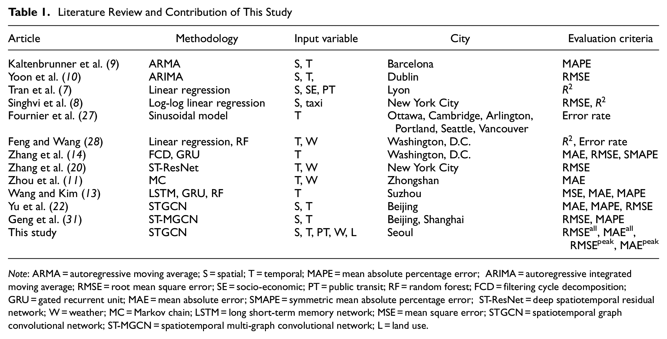
Note: ARMA = autoregressive moving average; S = spatial; T = temporal; MAPE = mean absolute percentage error; ARIMA = autoregressive integrated moving average; RMSE = root mean square error; SE = socio-economic; PT = public transit; RF = random forest; FCD = filtering cycle decomposition; GRU = gated recurrent unit; MAE = mean absolute error; SMAPE = symmetric mean absolute percentage error; ST-ResNet = deep spatiotemporal residual network; W = weather; MC = Markov chain; LSTM = long short-term memory network; MSE = mean square error; STGCN = spatiotemporal graph convolutional network; ST-MGCN = spatiotemporal multi-graph convolutional network; L = land use.

Methodology

GCN

GCN was first proposed to apply the convolutional neural network (CNN) to the graph structure ( 34 ). GCN solves the problem by representing the data as a graph $G = (V, E, X, A)$ with nodes $V \in R^{n}$ and edges E. Each node $v_{i} \in V$ is described with a feature vector $x_{i} \in R^{p}$ in feature matrix $X \in R^{N \times p}$ , and the relationship between the nodes is defined by adjacency matrix $A \in R^{N \times N}$ , which means that $a_{ij} \in A$ indicates the association within the nodes $v_{i}$ and $v_{j}$ . Degree matrix $D \in R^{N \times N}$ is a diagonal matrix that consists of the sum of elements in each row of A. ( $D_{ii} = \sum_{j} A_{ij}$ ) GCN transforms a graph G to a normalized graph Laplacian L to proceed a spectral convolution. Laplacian L of a graph is defined below:

L = I_{N} - D^{- \frac{1}{2}} A D^{- \frac{1}{2}} = U Λ U^{T}

(1)

Here, $I_{N}$ denotes an $N \times N$ identity matrix, and U is the eigenvector matrix of L with the corresponding eigenvalue matrix $Λ$ . Eigenvector matrix and eigenvalue matrix are used to express a spectral convolution on graphs, which is defined as a multiplication between a vector $x \in R^{N}$ and a filter $g_{θ}$ parameterized by $θ \in R^{N}$ .

g_{θ}^{*} x = U g_{θ} (Λ) U^{T} x

(2)

Finding the eigenvector and the eigenvalue of a matrix is a computationally expensive operation; so, in practice, graph convolution is approximated to Chebyshev polynomials ( 35 ). Approximation includes Chebyshev coefficients $θ' \in R^{K}$ , Chebyshev polynomials $T_{k} (x)$ up to the Kth order, and rescaled eigenvalue matrix $Λ'$ , where $Λ' = 2 Λ / λ_{\max} - I_{N}$ .

g_{θ'} (Λ) \approx \sum_{k = 0}^{K} θ_{k}^{'} T_{k} (Λ')

(3)

Graph Laplacian L also is transformed to L′, with $L' = 2 L / λ_{\max} - I_{N}$ . Then, the spectral graph convolution is approximated to polynomials ( 36 ).

g_{θ^{'}} * x \approx \sum_{k = 0}^{K} θ_{k}^{'} T_{k} (L^{'}) x = \sum_{k = 0}^{K} θ_{k}^{'} U Λ^{k} U^{T} x = \sum_{k = 0}^{K} θ_{k}^{'} L^{k} x

(4)

In the linear formulation of GCN, $λ_{\max}$ is approximated by a value of two, and the neural network parameter is expected to learn this value during training ( 34 ). ${(- 1)}^{k} θ_{k}^{'}$ also converges to a single value as the parameter is shared through the whole graph. Using these properties, the approximated version of a polynomial expression can be stated as shown below:

g_{θ'} * x \approx θ_{0}^{'} x + θ_{1}^{'} (L - I_{N}) = θ_{0}^{'} x - θ_{1}^{'} D^{- \frac{1}{2}} A D^{- \frac{1}{2}} x \approx θ (I_{N} + D^{- \frac{1}{2}} A D^{- \frac{1}{2}}) x

(5)

The term $I_{N} + D^{- \frac{1}{2}} A D^{- \frac{1}{2}}$ is converted to ${\tilde{D}}^{- \frac{1}{2}} \tilde{A} {\tilde{D}}^{- \frac{1}{2}}$ with $\tilde{A} = A + I_{N}$ and ${\tilde{D}}_{ii} = \sum_{j} {\tilde{A}}_{ij}$ to avoid exploding/vanishing gradients and numerical instabilities. This matrix calculation proceeds in each hidden layer H of GCN. The lth hidden layer, that is, $H^{l}$ , is a function of the (l−1)th hidden layer $H^{l - 1}$ , (l−1)th weight matrix $W^{l - 1}$ , (l−1)th bias matrix $b^{l - 1}$ , and adjacency matrix A, denoted as $H^{l} = σ (A H^{l - 1} W^{l - 1} + b^{l - 1})$ . The term $σ$ is an activation function between layers, such as a rectified linear unit or a sigmoid function. Using the polynomial approximation, the equation is stated in normalized form.

H^{l} = σ ({\tilde{D}}^{- \frac{1}{2}} \tilde{A} {\tilde{D}}^{- \frac{1}{2}} H^{l - 1} W^{l - 1} + b^{l - 1})

(6)

STGCN

With the developed GCN hidden layers, the STGCN framework is constructed for the prediction problem. The STGCN framework used in this study is discussed in detail (Figure 1). Recent studies introduce the idea of STGCN containing several STGCN blocks and a fully-connected output layer ( 22 , 37 ). The STGCN block contains a spatial block that represents the spatial relationship and has two gated temporal convolutional blocks in both ends. It helps to capture the prominent spatial and temporal features of the system simultaneously. The time blocks are based on a gated CNN, and the spatial blocks are constructed with GCN. The nonlinear gates within the gated CNN infer the information in the stacked temporal layers ( 37 ). Weight and bias matrix are the learnable parameters of this neural network structure during the training process in each layer whereas the adjacency matrix remains unchanged. It is designed to process structured time-series data, such as station-based bike-sharing demand, and it is good at predicting future demand. In this research, the temporal and spatial blocks have 64 and 62 channels, respectively.

Figure 1.

STGCN framework.

The STGCN models consist of two matrices: the adjacency matrix and the node feature matrix. The adjacency matrix contains the data that represent the relationship between nodes, such as the distance between stations. It can be predefined to implement pairwise correlations or connectivity between nodes ( 26 , 33 ). Information about each station’s circumstances is described in the node feature matrix, which includes past public bike-share demand patterns, weather conditions, day of the week, land-use purposes, and records of the use of public transportation.

The first model is a GCN with a feature matrix that contains past rental and return patterns with weather, holiday, and land-use features. Based on this model, other models that contain data concerning the use of public transportation were built. GCN-S and GCN-B are subway boarding record data and bus usage information, respectively. GCN-SB contains hourly usage data for both subways and buses.

Evaluation Criteria

Table 1 describes various evaluation criteria applied to the models. To compare the models and analyze sensitivity, two different aspects of the evaluation metrics are designed to focus both on overall time steps and peak hours. Root mean square error (RMSE) and mean absolute error (MAE) are used as the evaluation metrics that represent the error in all stations, and they are calculated as follows:

RMS E^{all} = \sqrt{\frac{1}{M^{h} \times N} \sum_{all i} \sum_{all j} {(y_{i^{h} j} - {\hat{y}}_{i^{h} j})}^{2}}

(7)

MA E^{all} = \frac{1}{M^{h} \times N} \sum_{all i} \sum_{all j} | y_{i^{h} j} - {\hat{y}}_{i^{h} j} |

(7)

where $M^{h}$ is the number of hourly time steps, N is the number of stations, and $y_{i^{h} j}$ and ${\hat{y}}_{i^{h} j}$ are the actual and predicted demand, respectively, at hourly time step $i^{h}$ and station j.

Little work has focused on the peak error. Owing to the nature of public bike-sharing systems, the total number of bikes remains almost constant. The capacity utilization rate of the system at the peak hour is relatively much higher than the rate at non-peak hours. Thus, it is necessary to focus on the error, especially at the peak hour. Therefore, the error during the period with the highest rental rate of the day should be compared. Both the predicted demand and the actual maximum demand during the day are calculated. RMSE and MAE also are used to compare the performances of the model at the peaks:

RMS E^{peak} = \sqrt{\frac{1}{M^{d} \times N} \sum_{all i^{d}} \sum_{all j} {(y_{i^{d} j} - {\hat{y}}_{i^{d} j})}^{2}}

(9)

MA E^{peak} = \frac{1}{M^{d} \times N} \sum_{all i^{d}} \sum_{all j} | y_{i^{d} j} - {\hat{y}}_{i^{d} j} |

(10)

where $M^{d}$ is the number of daily time steps, N is the number of stations, and $y_{i^{d} j}$ and ${\hat{y}}_{i^{d} j}$ are the actual and the predicted daily peak demand at daily time step $i^{d}$ and station j, respectively.

Empirical Analysis

Figure 2 shows the flow chart of the empirical analysis used in this study, consisting of three parts: the first part processes the datasets to fit the STGCN model, the second part contains the prediction model of the STGCN, and the last part compares their accuracy. Details in each process and datasets are described in the following sections.

Figure 2.

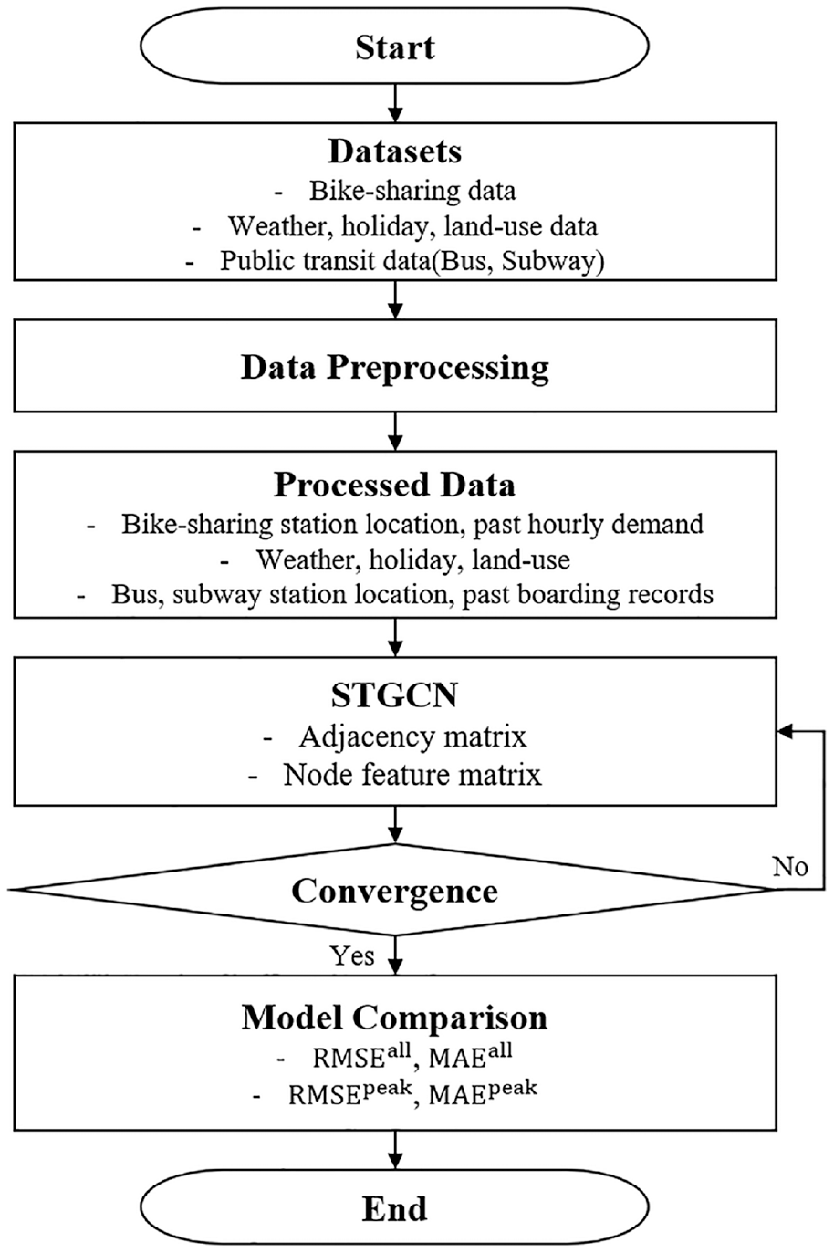
Process of empirical analysis.

Description of Data

This section describes five types of data used in this paper. All of the data are obtained from the Seoul Metropolitan Government of Korea and the Seoul Facilities Corporation database. Figure 3 presents the data that contain various characteristics of bike-sharing systems. The first data type is about bike-sharing stations. The data contain the station ID, the station name and address, and the capacity of the bike station. The second data type is the bike-sharing transaction data. The rental time, rental location, returning time, and return location are recorded for the public bike-sharing system. The third data type is the purpose for which the land is used where each bike station is located. These data indicate whether the parcel is a general commercial district, a residential district, or a natural green district. The fourth data type is hourly weather data, including wind speed, temperature, and rainfall. The last data type is about the usage of public transportation. The data show the number of passengers who board and alight at each subway station and at each bus stop.

Figure 3.

Data description.

There are two types of bike-sharing systems. Station-based bike-sharing systems need docking stations, and users need to rent from or return at the station; however, in a relatively new free-floating bike-sharing system, bikes can be locked to anywhere or even left standalone. Seoul public bike-sharing services are based on station-based systems. The site of the study is Yeouido-dong, Yeongdeungpo-gu, Seoul, South Korea. The selected area contains commercial, residential, and green areas that are evenly distributed with various characteristics of bike-sharing usage coexisting. It is known to have a particular rental pattern according to the hour of the day. There are only 31 stations in Yeouido-dong, but a total of 1,540 stations reside in Seoul. Figure 4 shows the locations of bike-sharing stations, bus stops, and subway stations. There are four subway stations and 57 bus stops within the study area. The data are collected at 1-h intervals, and 300,759 trips are collected over 131 days from March 1 to July 9, 2019. In this period, 63.41 rentals, on average, are made per hour at each rental office. Public transit data in the area contain an average of 193,266 subway trips and 117,728 bus trips per day. Among the collected data, 85% is used for the training/validation set and 15% is used for testing. A training and validation process is conducted to prevent the overfitting of the model.

Figure 4.

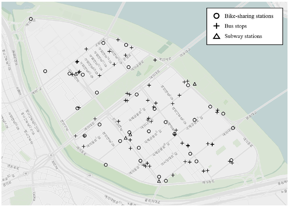
Locations of bike-sharing stations, bus stops, and subway stations in Yeouido-dong, Seoul, South Korea.

Preprocessing of Data

This section covers the process of preprocessing raw data to create the data needed for the experiment. Several matrices are created for use as an adjacency matrix and feature matrix by processing exogenous variables and public transport data, as well as the data related to bike-sharing. First, the data related to bike rental stations are compiled, and they consist of the Euclidean distance between each bike station and the data concerning the use of each parcel of land. Second, the origin–destination (OD) matrix of past demand shows that the past rental pattern for bikes and the observed demand matrix for each rental shop are arranged. Third, with the data related to public transit, the matrices contain boarding and alighting records from four subway stations and 57 bus stations within the geographical scope. Exogenous variables, such as weather and holidays, are modified to fit the input structure for the neural network. Other exogenous variables, such as holiday events and land-use data, are converted into binary variables, and weather conditions, including temperature, wind, and rainfall, are normalized with the min–max normalization method. The normalization process is useful because the model converges quickly to the optimum. Also, the maximum and minimum values are included to rescale the original value.

Adjacency and Node Feature Matrices

Four adjacency matrices are designed to reflect the relationship between bike-sharing stations and related characteristics. First, an identity matrix is constructed with the main diagonal having a value of one and off-diagonal entries assigned as zero. It represents the disconnected graph, which is used as a baseline model because it assumes there is no relationship between nodes. Second, the distance matrix is a matrix that reflects the Euclidean distance between the bike rental stations. The first law of geography tells us that everything is related to everything else, but objects near each other are more related than others that are far apart ( 38 ). The distance matrix is used to represent this geographical characteristic in bike-sharing stations. Third, the minimum public transit distance matrix considers the ratio of the Euclidean distance between each bike station, subway station, and bus stop to reflect how far the bike rental station is from the public transportation stop. Last, the OD matrix shows the rental and returns patterns. All of the matrices mentioned are normalized when they are used in the model.

The node feature matrices are designed to reflect the characteristics of each dataset by time zone and bike-sharing stations. First, the past rental and return demand patterns are included, and the values within the matrices are scaled by min–max normalization, and minimum and maximum values are included to represent each station’s rental scale. Also, it includes weather information, such as wind, temperature, rain, and land use. The subway and bus transaction matrix records the data from the subway stations and bus stops in Yeouido-dong. It is created by matrix multiplication of the matrix representing the distance from each bike rental station to the subway station and the boarding and alighting data at each subway station and taking the reciprocal value of each element.

Comparison of the Models

This section describes the models including five baseline time-series prediction models and GCN models developed with different adjacency and feature matrices. The models that are used for comparison are described as follows. (i) The historical average calculates the predicting demand of the next hour on the average of historical demands for the previous hours at each station. (ii) If the predicted values have a pattern of a seasonal factor, ARIMA separates the signal from the noise and deduces the signal in the future to make predictions. (iii) Exponential smoothing (ETS) was proposed in the late 1950s and it computes a weighted average over all observations in the input time series dataset ( 39 ). (iv) The non-parametric time series (NPTS) predicts the future distribution of a given period by sampling past observations; it is especially useful when the values are zero-inflated. (v) RF was first introduced in 2001 ( 40 ); it is a combination of decision tree predictors in which each tree relies on the independently sampled random vector; it is known for its robustness to noise and for working exceptionally well in short intervals of time ( 13 ). Five benchmark models are formulated with hourly weather data (temperature, wind, rainfall), holiday data, and land-use data. As described, there are four GCN models with different adjecency matrices of identity, distance, public transit distance, and OD matrix and other four models of GCN, GCN-S, GCN-B, and GCN-SB. In each model, different variables are included in the used node feature matrix.

Model Implementation

Empirical analysis with such different models is conducted with NVIDIA Tesla V100 SXM2 and 32 GB memory. In making predictions with the ARIMA, ETS, and NPTS models, Amazon forecast, the machine learning tool for predicting data with historical time-series data and additional exogenous variables, is used. Prediction using the RF model is tested experimentally and visualized using the statistical software R with “RandomForest.” The GCN models were based on the Pytorch 1.4.0, and the mean square error loss is used as the loss function. The adaptive moment estimation (ADAM) optimizer, first proposed in 2015, is used as the optimizer ( 41 ). ADAM continuously gives the weight momentum, allowing it to escape from the local solution. It also improves performance by adjusting the hyperparameters through a grid search. The batch size is varied from 50 to 150 and the learning rate is varied from 0.0005 to 0.01 to identify an appropriate value. An optimal number of epochs (i.e., 100) is determined through several experiments to avoid over-fitting and under-fitting problems.

Results and Discussion

This section covers the results of several models and each model is optimized by hyperparameters, such as the learning rate and epochs. Four metrics are selected as performance measures. Overall, the results show that the error of the whole period and the peak show different aspects. However, it is necessary to predict demand in peak hours accurately due to the nature of shared services. So, it is necessary to focus on the criteria associated with the peak. The results of the evaluation are assessed in two different ways: (i) the effects of the different adjacency matrices, and (ii) public transit data as node features. Multiple iterations are performed for each model.

Effects of Adjacency Matrix

The efficiency of the model is compared with different, predefined adjacency matrices. Embedding information primarily into the graphs is known to provide leverage for accurate forecasting ( 31 ). To determine the effect of the adjacency matrix, the models are examined experimentally using the same conditions. Table 2 shows the testing results of the STGCN model using various adjacency matrices on the test dataset. A comprehensive comparison with the error bar in Figure 5 indicates the efficiency and stability of the models. When considering RMSE^all in this experiment, RF shows the best performance and NPTS has the worst performance among the baseline models. RF does not do a good job of predicting peak values, but GCN using the distance matrix is good at predicting peak-hour demand. However, the RF model has a lower peak error value than GCN with the identity matrix. The GCN models definitively show better performance in predicting demand than the five baseline models. The indicators for observing errors at the peak fit well when the GCN model is used. This implies that GCN that contains a graphical structure is more advantageous in predicting demand than the other baseline models. Among the GCN models, the model that uses the OD matrix as the adjacency matrix shows the best performance for all indicators. Prior research shows that GCN’s performance depends on the hidden pairwise correlation between the nodes and the model with the historical usage patterns better reflects the connectivity than the model with the geographical distance ( 26 ).

Table 2.

Comparison of the Efficiencies of Models with Different Adjacency Matrices

Models	Adjacency matrix	RMSE^all	MAE^all	RMSE^peak	MAE^peak
HA	—	4.281	2.063	11.323	8.142
ARIMA	—	4.464	2.246	13.004	9.071
ETS	—	4.081	2.109	10.050	7.237
NPTS	—	4.486	2.304	14.422	10.339
RF	—	3.954	2.115	9.161	6.131
GCN	Identity matrix	3.879	2.128	9.302	6.319
	Distance matrix	3.991	2.164	9.525	6.542
	Public transit distance matrix	3.963	2.147	9.549	6.541
	OD matrix	3.704	2.008	9.051	6.149

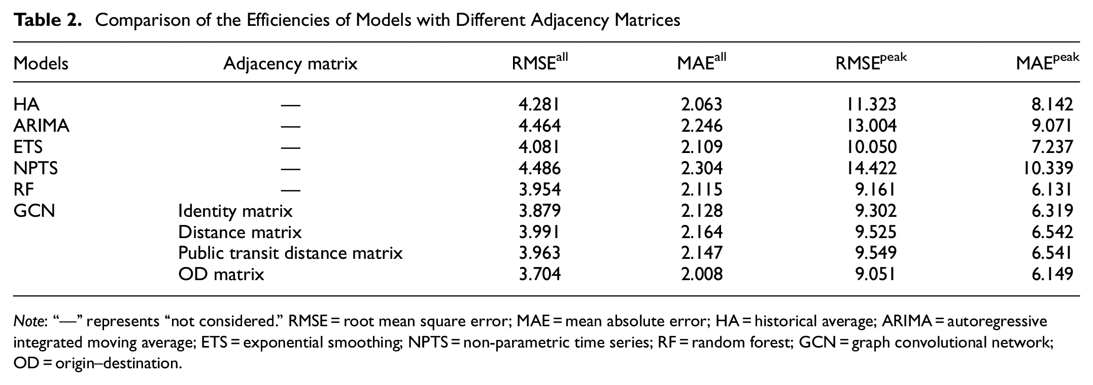
Note: “—” represents “not considered.” RMSE = root mean square error; MAE = mean absolute error; HA = historical average; ARIMA = autoregressive integrated moving average; ETS = exponential smoothing; NPTS = non-parametric time series; RF = random forest; GCN = graph convolutional network; OD = origin–destination.

Figure 5.

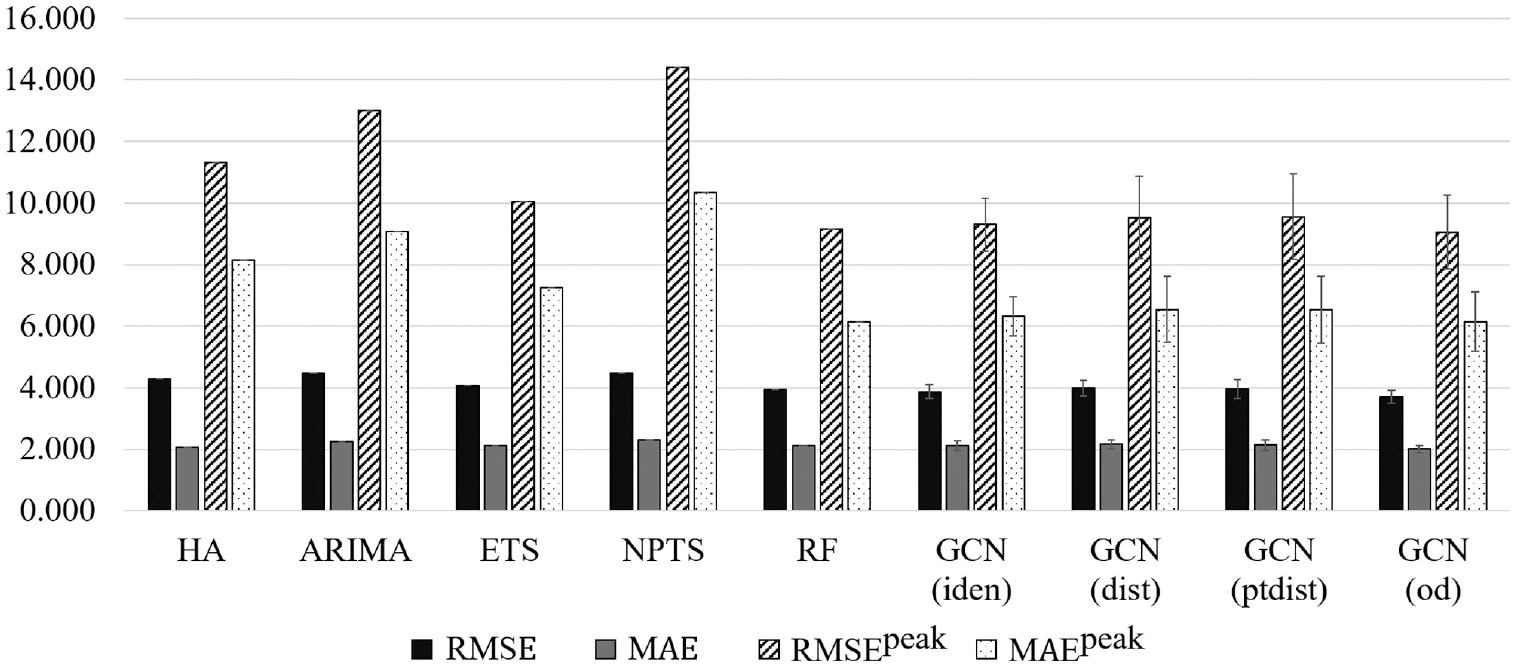
Comparison of the efficiencies of models with different adjacency matrices.

The Pearson correlation of the OD matrix is used to determine the correlation of the demands between stations. Figure 6 shows the pairwise correlation of bike-sharing demands in some stations. An observable and notable pattern is found in which some stations are highly correlated with each other but others are not. As the correlations between these bike-sharing stations can be defined, a model that reflects this relationship can contribute to accurate predictions of demand.

Figure 6.

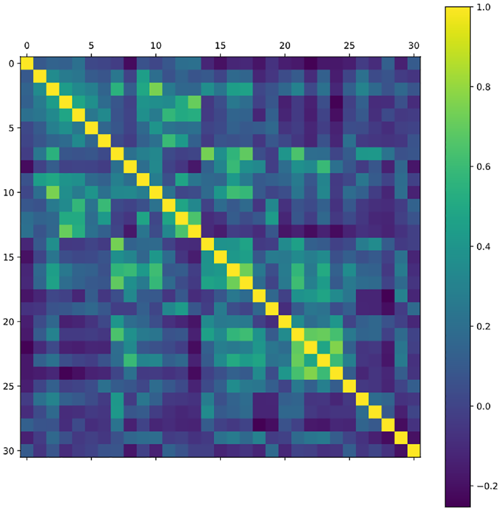
Correlation matrix for the stations that used historical demand for rental bike-sharing.

Effects of Public Transit Data in the Node Feature Matrix

Public bike-sharing demand is said to be related to public transportation. An experiment is conducted to corroborate the effect of public transportation data, including bus and subway usage data, as node features. The exogenous variables include weather, holidays, and land use for equal comparison. (Table 3, Figure 7) As putting public transportation use data and past demand patterns into the adjacency matrix at the same time may lead to a redundancy problem, the distance matrix is used as the adjacency matrix for comparison. For the RMSE^all of the whole period, the GCN model excluding public transportation data had the best accuracy. However, the accuracy of GCN-S that includes the subway, GCN-B, and GCN-SB is improved in that order from the aspect of MAE^all. In particular, the more public transportation data put into the matrix, and the more bus data than subway data, the more accurate the predictive model is. However, comparing peak periods, RMSE^peak and MAE^peak are lower in the GCN-B model with bus data than in the GCN model without public transportation data. The GCN-S model, which reflects the subway boarding and alighting data, is slightly less capable of predicting the peak demand. The RMSE of the prediction model was compared for each bike-sharing station. The RMSE improvement of the GCN-S model compared with the GCN of the nearest 10% bike station to the subway is 2.95% lower than that of the other bike stations. The RMSE improvement of the GCN-B model for bus is 3.61% lower than that of the other stations. Even when both bus and subway data were considered, it improved by 3.28%. This may imply that public transit usage records help in predicting bike-sharing demand.

Table 3.

Comparison of the Efficiencies of Models with a Different Node Feature Matrix

Models	RMSE^all	MAE^all	RMSE^peak	MAE^peak
GCN	3.991	2.164	9.525	6.542
GCN-S	4.240	2.131	10.524	7.136
GCN-B	4.146	2.116	8.895	6.073
GCN-SB	4.177	2.108	9.704	6.672

Note: RMSE = root mean square error; MAE = mean absolute error; GCN = graph convolutional network; S = subway; B = bus; SB = subway and bus.

Figure 7.

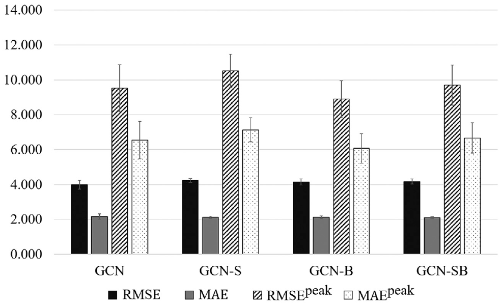
Effects of public transit data in the node feature matrix.

There are two possible reasons for the effects of public transit data in the node feature matrix. The first reason is that the rate of transferring the trip between bike-sharing and buses is much higher than the rate of transfer to subways. Owing to the regional characteristics of the study area, higher demands are observed in residential areas than in other areas. An additional analysis is performed using bike-sharing data and data from the public transit transferring mileage system. The matched data are used between smart card data and bike-sharing data from January to June 2017 in Yeouido-dong. The ratio of bus-connected bike-sharing trips to that of subway-connected trips is 1.38:1. However, the ratio of the number of boarding and alighting buses to that of subways is about 0.609:1. From the values, the bike-sharing transfer ratio of buses is 2.26 times higher than the ratio of the subway. The intermodal transfer rate with the bike-sharing system is higher in buses than in the subway, which implies better connectivity between the two systems. The second is the difference in accessing the bike-sharing stations from the bus and the subway. Figure 4 shows that the distribution of bus stops is much denser than that of subway stations, with bus stops also being closer to the bike rental stations. The average distances from each bus stop and subway station to the nearest bike rental station are 0.127 and 0.363 km, respectively. Bike-sharing users certainly have more access to bus stops than to subway stations.

Conclusions and Future Work

In recent years, the number of people using public bikes has increased. The accurate station-wise prediction of demand enables the high quality of service; thus, it has emerged as a critical issue. Previous works focused on improving the accuracy of the predicted demand for bike-sharing, and some of them used the GCN framework. GCN was introduced to directly reflect the graphical structure of data into the neural network. The STGCN framework was proposed to embed the spatiotemporal characteristics and applied to diverse domains, including the predictions of traffic flow. This study focuses on the accurate prediction of the future demand for bike-sharing, especially at the peak.

Recent studies related to predicting the extent of bike-sharing research with GCN have focused on increasing the overall accuracy by diversifying the adjacency matrix of the GCN structure, thereby enabling dynamic reflection of the adjacency matrix and reanalyzing the graph network with the correlation between nodes. It is essential to accurately forecast the overall future demand; however, it is much more critical to predict the value at the peak, that is, when people rent the most. In this study, RMSE^peak and MAE^peak are introduced as indicators that can be used to evaluate the peak error and determine whether or not the model predicts the peak value well. Several predefined adjacency matrices are used, including public transportation data, in the STGCN framework and their effects compared.

Results showed that, in predicting the future demand for bike-sharing, the GCN models eminently perform better than the five baseline models. Also, various adjacency matrices were applied and the results indicated that the adjacency matrix that reflected the previous OD pattern provided better predictions than the model that reflected the geographical distance or the model that reflected the reciprocal distance to the public transit stations. Throughout the results above, the association between public transport and public bike-sharing system was identified. It turned out that the model, including the bus arrival and departure records, had better accuracy. This result may have occurred because the bus has a higher transfer ratio to a bike than to a subway. Another reason could be the average distance from a public transportation station to a bike station. The average distance between bus and bike stops is only one-third of the average distance between subway stations and bike stops. Therefore, the results of this study indicate that including public transit data with greater relationships helps provide accurate predictions.

This study has limitations in potential unmet demand that was not considered in the data. Even if there were a potential unmet demand, the historical demand data could not include it; thus, the historical demand data are underestimated. Also, as this study uses only the predefined adjacency matrix, it is hard to reflect the dynamically changing graph structure. If the model can reflect real-time relationships or correlations between stations, it may be efficient in dealing with sudden changes or failures. The model that reflects changing graph structures and changing hidden correlations could be investigated further. The connection between bike-sharing and public transportation and its composition are expected to be related to regional characteristics. Therefore, future work should include analyses of various regions. An indicator of the relationship between public transit and bike-sharing, that is, how similarly distributed the public transit stations are to bike stations, should be also developed for accurate predictions of bike-sharing demand.

Footnotes

Acknowledgements

The authors acknowledge the support from the HPC Support Project funded by the Ministry of Science and ICT and NIPA.

Author Contributions

The authors confirm contribution to the paper as follows: study conception and design: J.-H. Cho, S.W. Ham, D.-K. Kim; data collection: J.-H. Cho; analysis and interpretation of results: J.-H. Cho, S.W. Ham, D.-K. Kim; draft manuscript preparation: J.-H. Cho, S.W. Ham. All authors reviewed the results and approved the final version of the manuscript.

Declaration of Conflicting Interests

The author(s) declared no potential conflicts of interest with respect to the research, authorship, and/or publication of this article.

Funding

The author(s) disclosed receipt of the following financial support for the research, authorship, and/or publication of this article: This research was supported by the Basic Science Research Program through the National Research Foundation of Korea funded by the Ministry of Science and ICT, Government of South Korea (NRF-2020R1F1A1074395).

References

Shaheen

Guzman

Zhang

Bikesharing in Europe, the Americas, and Asia. Transportation Research Record: Journal of the Transportation Research Board, 2010. 2143: 159–167. https://doi.org/10.3141/2143-20.

Chiariotti

Pielli

Zanella

Zorzi

A Dynamic Approach to Rebalancing Bike-Sharing Systems. Sensors (Switzerland), Vol. 18, No. 2, 2018, pp. 1–22. https://doi.org/10.3390/s18020512.

Caggiani

Camporeale

Ottomanelli

Szeto

W. Y.

A Modeling Framework for the Dynamic Management of Free-Floating Bike-Sharing Systems. Transportation Research Part C: Emerging Technologies, Vol. 87, 2018, pp. 159–182. https://doi.org/10.1016/j.trc.2018.01.001.

Liu

Szeto

W. Y.

S. C.

A Static Free-Floating Bike Repositioning Problem with Multiple Heterogeneous Vehicles, Multiple Depots, and Multiple Visits. Transportation Research Part C: Emerging Technologies, Vol. 92, 2018, pp. 208–242. https://doi.org/10.1016/j.trc.2018.02.008.

Pal

Zhang

Free-Floating Bike Sharing: Solving Real-Life Large-Scale Static Rebalancing Problems. Transportation Research Part C: Emerging Technologies, Vol. 80, 2017, pp. 92–116. https://doi.org/10.1016/j.trc.2017.03.016.

Hulot

Aloise

Jena

S. D.

Towards Station-Level Demand Prediction for Effective Rebalancing in Bike-Sharing Systems. Proc., ACM SIGKDD International Conference on Knowledge Discovery and Data Mining, London, Association for Computing Machinery, New York, NY, 2018, pp. 378–386. https://doi.org/10.1145/3219819.3219873.

Tran

T. D.

Ovtracht

D’Arcier

B. F.

Modeling Bike Sharing System Using Built Environment Factors. Procedia CIRP, Vol. 30, 2015, pp. 293–298. https://doi.org/10.1016/j.procir.2015.02.156.

Singhvi

Frazier

P. I.

Henderson

S. G.

O’Mahony

Shmoys

D. B.

Woodard

D. B.

Predicting Bike Usage for New York City’s Bike Sharing System. AAAI Workshop—Technical Report, Vol. WS-15-06, 2015, pp. 110–114.

Kaltenbrunner

Meza

Grivolla

Codina

Banchs

Urban Cycles and Mobility Patterns: Exploring and Predicting Trends in a Bicycle-Based Public Transport System. Pervasive and Mobile Computing, Vol. 6, No. 4, 2010, pp. 455–466. https://doi.org/10.1016/j.pmcj.2010.07.002.

10.

Yoon

J. W.

Pinelli

Calabrese

Cityride: A Predictive Bike Sharing Journey Advisor. Proc., 2012 IEEE 13th International Conference on Mobile Data Management, MDM 2012, Bengaluru, India, IEEE, 2012, pp. 306–311. https://doi.org/10.1109/MDM.2012.16.

11.

Zhou

Wang

Zhong

Tan

A Markov Chain Based Demand Prediction Model for Stations in Bike Sharing Systems. Mathematical Problems in Engineering, Vol. 2018, 2018, pp. 1–8. https://doi.org/10.1155/2018/8028714.

12.

Park

H. C.

Kang

Kho

S. Y.

Kim

D. K.

Investigation of Effects of Inherent Variation and Spatiotemporal Dependency on Urban Travel-Speed Prediction. Journal of Transportation Engineering Part A: Systems, Vol. 146, No. 5, 2020, pp. 1–9. https://doi.org/10.1061/JTEPBS.0000341.

13.

Wang

Kim

Short-Term Prediction for Bike-Sharing Service Using Machine Learning. Transportation Research Procedia, Vol. 34, 2018, pp. 171–178. https://doi.org/10.1016/j.trpro.2018.11.029.

14.

Zhang

Shen

Zhao

Yang

G. H.

Time Series Forecasting Using GRU Neural Network with Multi-Lag after Decomposition. Lecture Notes in Computer Science (including subseries Lecture Notes in Artificial Intelligence and Lecture Notes in Bioinformatics), Vol. 10638 LNCS, No. 1, 2017, pp. 523–532. https://doi.org/10.1007/978-3-319-70139-4_53.

15.

Kim

E. J.

Park

H. C.

Kho

S. Y.

Kim

D. K.

A Hybrid Approach Based on Variational Mode Decomposition for Analyzing and Predicting Urban Travel Speed. Journal of Advanced Transportation, Vol. 2019, 2019, pp. 1–12. https://doi.org/10.1155/2019/3958127.

16.

Campbell

A. A.

Cherry

C. R.

Ryerson

M. S.

Yang

Factors Influencing the Choice of Shared Bicycles and Shared Electric Bikes in Beijing. Transportation Research Part C: Emerging Technologies, Vol. 67, 2016, pp. 399–414. https://doi.org/10.1016/j.trc.2016.03.004.

17.

Zhang

Liu

Yang

Short-Term Prediction of Bike-Sharing Usage Considering Public Transport: A LSTM Approach. Proc., 21st International IEEE Conference on Intelligent Transportation Systems, ITSC, Maui, HI, Vol. 2018, No. 61773293, 2018, pp. 1564–1571. https://doi.org/10.1109/ITSC.2018.8569726.

18.

Kapuku

Kho

S. Y.

Kim

D. K.

Cho

S. H.

Modeling the Competitiveness of a Bike-Sharing System Using Bicycle GPS and Transit Smartcard Data. Transportation Letters, 2020, online published. https://doi.org/10.1080/19427867.2020.1758389.

19.

Song

Huang

Investigating Complementary and Competitive Relationships between Bikeshare Service and Public Transit: A Spatial-Temporal Framework. Transportation Research Record: Journal of the Transportation Research Board, 2020. 2674: 260–271. https://doi.org/10.1177/0361198119899389.

20.

Zhang

Zheng

Deep Spatio-Temporal Residual Networks for Citywide Crowd Flows Prediction. Proceedings of the AAAI Conference on Artificial Intelligence, Vol. 31, No. 1, 2017, pp. 1655–1661.

21.

Huang

Qiao

Peng

Guo

A Bimodal Gaussian Inhomogeneous Poisson Algorithm for Bike Number Prediction in a Bike-Sharing System. IEEE Transactions on Intelligent Transportation Systems, Vol. 20, No. 8, 2019, pp. 2848–2857. https://doi.org/10.1109/TITS.2018.2868483.

22.

Yin

Zhu

Spatio-Temporal Graph Convolutional Networks: A Deep Learning Framework for Traffic Forecasting. Proc., 27th IJCAI International Joint Conference on Artificial Intelligence, Stockholm, Sweden, Vol. 2018, AAAI Press, 2018, pp. 3634–3640. https://doi.org/10.24963/ijcai.2018/505.

23.

Lee

Sohn

Forecasting Road Traffic Speeds by Considering Area-Wide Spatio-Temporal Dependencies Based on a Graph Convolutional Neural Network (GCN). Transportation Research Part C: Emerging Technologies, Vol. 114, 2020, pp. 189–204. https://doi.org/10.1016/J.TRC.2020.02.013.

24.

Zhang

Zheng

DNN-Based Prediction Model for Spatio-Temporal Data. Proc., ACM SIGSPATIAL International Conference on Advances in Geographic Information Systems, Burlingame, CA, Association for Computing Machinery, New York, NY, 2016, p. 92.

25.

Sathishkumar

V. E.

Cho

A Rule-Based Model for Seoul Bike Sharing Demand Prediction Using Weather Data. European Journal of Remote Sensing, Vol. 53, 2020, pp. 166–183. https://doi.org/10.1080/22797254.2020.1725789.

26.

Kim

T. S.

Lee

W. K.

Sohn

S. Y.

Graph Convolutional Network Approach Applied to Predict Hourly Bike-Sharing Demands Considering Spatial, Temporal, and Global Effects. PLoS One, Vol. 14, No. 9, 2019, pp. 1–16. https://doi.org/10.1371/journal.pone.0220782.

27.

Fournier

Christofa

Knodler

M. A.

A Sinusoidal Model for Seasonal Bicycle Demand Estimation. Transportation Research Part D: Transport and Environment, Vol. 50, 2017, pp. 154–169. https://doi.org/10.1016/j.trd.2016.10.021.

28.

Feng

Wang

A Forecast for Bicycle Rental Demand Based on Random Forests and Multiple Linear Regression. Proc., 16th IEEE/ACIS International Conference on Computer and Information Science, ICIS 2017, Wuhan, China, IEEE, 2017, pp. 101–105. https://doi.org/10.1109/ICIS.2017.7959977.

29.

Ham

S. W.

Cho

J.-H.

Park

Kim

D.-K.

Spatiotemporal Demand Prediction Model for E-Scooter Sharing Services with Latent Feature and Deep Learning. Transportation Research Record: Journal of the Transportation Research Board, 2021. https://doi.org/10.1177/03611981211003896.

30.

Scarselli

Gori

Tsoi

A. C.

Hagenbuchner

Monfardini

The Graph Neural Network Model. IEEE Transactions on Neural Networks, Vol. 20, No. 1, 2009, pp. 61–80. https://doi.org/10.1109/TNN.2008.2005605.

31.

Geng

Wang

Zhang

Yang

Liu

Spatiotemporal Multi-Graph Convolution Network for Ride-Hailing Demand Forecasting. Proceedings of the AAAI Conference on Artificial Intelligence, Vol. 33, 2019, pp. 3656–3663. https://doi.org/10.1609/aaai.v33i01.33013656.

32.

Guo

Lin

Feng

Song

Wan

Attention Based Spatial-Temporal Graph Convolutional Networks for Traffic Flow Forecasting. Proceedings of the AAAI Conference on Artificial Intelligence, Vol. 33, 2019, pp. 922–929. https://doi.org/10.1609/aaai.v33i01.3301922.

33.

Lin

Peeta

Predicting Station-Level Hourly Demand in a Large-Scale Bike-Sharing Network: A Graph Convolutional Neural Network Approach. Transportation Research Part C: Emerging Technologies, Vol. 97, 2018, pp. 258–276. https://doi.org/10.1016/j.trc.2018.10.011.

34.

Kipf

T. N.

Welling

Semi-Supervised Classification with Graph Convolutional Networks. Proc., 5th International Conference on Learning Representations, ICLR 2017—Conference Track Proceedings, Toulon, France, 2019, pp. 1–14.

35.

Hammond

D. K.

Vandergheynst

Gribonval

Wavelets on Graphs via Spectral Graph Theory. Applied and Computational Harmonic Analysis, Vol. 30, No. 2, 2011, pp. 129–150. https://doi.org/10.1016/j.acha.2010.04.005.

36.

Defferrard

Bresson

Vandergheynst

Convolutional Neural Networks on Graphs with Fast Localized Spectral Filtering. Advances in Neural Information Processing Systems, 2016, pp. 3844–3852. https://doi.org/10.1016/j.commatsci.2018.05.018.

37.

Xiao

Wang

Zhang

Demand Prediction for a Public Bike Sharing Program Based on Spatio-Temporal Graph Convolutional Networks. Multimedia Tools and Applications, 2020, online published. https://doi.org/10.1007/s11042-020-08803-y.

38.

Tobler

W. R.

A Computer Movie Simulating Urban Growth in the Detroit Region. Economic Geography (Issue Supplement 1: Proceedings, International Geographical Union. Commission on Quantitative Methods), Vol. 11, No. 46, 1970, pp. 234–240. https://doi.org/10.1126/science.11.277.620.

39.

Holt

C. C.

Forecasting Seasonals and Trends by Exponentially Weighted Moving Averages. International Journal of Forecasting, Vol. 20, No. 1, 2004, pp. 5–10. https://doi.org/10.1016/j.ijforecast.2003.09.015.

40.

Breiman

Random Forests. Machine Learning, Vol. 45, No. 1, 2001, pp. 5–32. https://doi.org/10.1023/A:1010933404324.

41.

Kingma

D. P.

J. L.

Adam: A Method for Stochastic Optimization. Proc., 3rd International Conference on Learning Representations, ICLR 2015—Conference Track Proceedings, Ithaca, NY, 2015, pp. 1–15.