Exploration of Maximum-to-Minimum Shifts in Generic Methods for Departure Time Choice Models

Abstract

Vickrey’s seminal departure time choice model is based on a penalty function which is a linear combination of travel time, earliness, and lateness. The original model depicts a single link from a single origin to a single destination, serving homogeneous travelers by a deterministic point-queue regime. Numerous variants of the basic model, relaxing one or more of these assumptions, have been used in a wide range of contexts. The equilibrium solution of the basic model can be computed directly by exact formula. Specific convergent methods have been proposed for certain variants. One of the troubling challenges in this model is the need for a generic iterative numeric approach, that may address complex models in which departure time choice is embedded. Natural candidates were shown to fail even on the basic model. In this paper we explore a fairly naive approach, where, in each iteration, demand is shifted from the maximum cost time interval to the minimum cost time interval. Results for the basic model are promising, demonstrating that, with a fixed shift, solutions converge to a deviation which is proportional to the shift size and that semi-adaptive or adaptive shift size may offer convergence to any desirable level of approximation of the exact equilibrium.

Departure time choice is one of the most critical factors affecting congestion in transportation networks. Many studies on this topic rely on schedule penalties, as introduced by Vickrey ( 1 ) in his seminal paper about the bottleneck model. Small ( 2 ) provides a thorough overview of the research that stemmed from the bottleneck model.

The basic model relies on many simplifying assumptions: all travelers depart from the same origin to the same destination, using their private cars to follow the same link, along which there exists a single bottleneck. The bottleneck operates as a deterministic point-queue with known capacity. Demand is also deterministic, as are travel times from the origin to the bottleneck and from the bottleneck to the destination. All travelers are homogenous in their desired arrival times, as well as the penalties they associate with 1 min of travel time/earliness/lateness. The basic model considers flows and departure times as continuous.

Extensions and variants of the model may incorporate for example: tolls ( 1 ); heterogeneity (3–5); discretized departure times ( 4 , 5 ); demand materialization stochasticity ( 6 ); network structure; mode choice; and so forth. The equilibrium solution of the basic model can be computed by exact formulas, see details below. Specific methods have been proposed for some of the above-mentioned variants. Nevertheless, when equilibrium of departure time choice is sought in association with a complex multi-modal network model, a generic method would be desirable. We consider a method to be “fully” generic (or generalizable) if it prescribes how to iteratively adjust departure time choices in view of the estimated generalized cost values by departure time, while treating the cost computation process as a black box. In other words, to be fully generic, the method should not rely on detailed insights into delay dynamics or the cost structure.

Mechanisms for adjusting choices in view of consequences are very typical in equilibrium models. In many equilibrium models, if adjustments are sufficiently small, almost any reasonable adjustment mechanism can lead to convergence. Surprisingly, this is not the case with the departure time choice model. Some “natural candidate” adjustment mechanisms exhibit dynamic instability and fail to converge regardless of step size, even on the basic model. (See additional details below.)

In addition to the computational concern, a behavioral concern is raised by these observations of unstable dynamics. If the instability is inherent to the model, rather than specific to the proposed adjustment mechanisms, then the usefulness of the model in describing reality should be questioned. Therefore, an urgent issue is to verify whether there exists at least one stable adjustment mechanism for the departure time choice model.

Most previous studies of the stability issue “only examined a finite number of dynamical systems for departure time choice but do not rule out the existence of an unknown stable one” ( 7 ). If travelers have complete information of the current day, including the departure and arrival cumulative flows, as well as sufficient understanding of the congestion mechanism to determine when the bottleneck is underused, then they can follow a two-stage decision process, planning their arrival time first, and choosing their departure time during the execution phase. Such behavior leads to stable dynamics ( 7 ), but the ability to generalize this sophisticated dynamic process for more complex situations is not trivial at all.

The good news presented in this paper is that perhaps not all hope is lost. Specifically, we show promising results obtained by a fairly simplistic adjustment scheme, applied to the basic model with discretized departure times. The adjustment process is based on demand shifts from the time interval with highest generalized cost to the time interval with the lowest generalized cost. This simple adjustment scheme can be implemented in principle with any “black-box” model that produces travel times for given departure rates, and in that sense the proposed approach has generalization potential to more complex models, beyond the basic model evaluated here. Computationally such an adjustment process may seem wasteful, as the effort of recomputing delays and generalized costs is performed numerous times. Behaviorally the max-to-min shift is probably not particularly similar to the change travelers make in their departure time choices from day to day in reality. Despite these limitations, we believe that the demonstration of convergence of one method may lead to developments of additional convergent methods, which will hopefully be more efficient computationally, more representative of real-life day-to-day dynamics, or both.

The remainder of this paper is organized as follows. First we provide background material, including a definition of the basic model. We then present the methods we tested, followed by the main numerical results. We end with conclusions and suggestions for future research.

Background

This paper focuses on the basic model for travelers’ departure time choices with discrete departure intervals, as defined by Ramadurai et al. ( 4 ). Consider N commuters planning to travel through a bottleneck with capacity S. They plan their departure times independently, but their delay at the bottleneck is determined by a deterministic point-queue. Deterministic travel times from the origin to the bottleneck and from the bottleneck to the destination can be ignored, for notational simplicity.

The modeling period is divided into M time intervals of duration $Δ t$ . Departure intervals are denoted by i, where $0 \leq i \leq M$ . The (continuous) number of departures during interval i is denoted by $r_{i}$ . Departure at the end of interval i leads to a delay of:

Q_{i} (r) = {[Q_{i - 1} (r) + (\frac{r_{i}}{S} - 1) \cdot Δt]}_{+}

(1)

where ${[x]}_{+} = \max (0, x)$ , and $Q_{0} = 0$ represents the delay at the beginning of the first interval $i = 1$ . Since all travelers wish to reach their destination at time $t^{*}$ , the resulting arrival time, earliness, and lateness are:

T_{i} (r) = i \cdot Δt + Q_{i} (r)

(2)

E_{i} (r) = {[t^{*} - T_{i} (r)]}_{+}

(3)

L_{i} (r) = {[T_{i} (r) - t^{*}]}_{+},

(4)

The generalized cost by departure time interval is:

C_{i} (r) = α \cdot Q_{i} (r) + β \cdot E_{i} (r) + γ \cdot L_{i} (r),

(5)

where $α$ reflects the value of travel time, $β$ is the penalty coefficient for earliness, and $γ$ is the penalty coefficient for lateness. At equilibrium, travelers depart only during intervals associated with minimum generalized cost, that is, the vector $r^{*}$ is an equilibrium solution if

r_{i}^{*} > 0 \Rightarrow C_{i} (r^{*}) = C^{*} (r^{*}),

(6)

where $C^{*} (r) = min_{i} C_{i} (r)$ is defined as the minimum cost over all departure times.

Ramadurai et al. ( 4 ) show that the equilibrium cost is uniquely determined by the inputs of this model (N, S, $t^{*}$ , $α$ , $β$ , $γ$ ); but, in general, there may be multiple vectors of departure rates that satisfy the equilibrium conditions. They further show that the deterministic model with homogenous (or heterogenous) travelers can be formulated as a variational inequality (VI) problem, and thus it can be solved by generic VI methods. Extensions of this approach to other variants of the model, for example, stochastic materialization of demand, have not been reported in the literature as far as we know.

To evaluate the proximity to equilibrium of a given vector of departure amounts, $r$ , two measures are used. The first is the potential defined by Gou et al. ( 5 ) as:

V (r) = \sum_{i = 1}^{M} \sum_{j = 1}^{M} r_{i} \cdot {[C_{i} (r) - C_{j} (r)]}_{+}^{2},

(7)

The second measure for equilibrium-proximity is the root mean square (RMS):

RMS (r) = \sqrt{\frac{\sum_{i = 1}^{M} r_{i} \cdot {[C_{i} (r) - C^{*} (r)]}^{2}}{N}}

(8)

Both measures are non-negative and obtain a value of zero if and only if the vector of departure amounts satisfies the equilibrium conditions. In principle, one of these two measures can be sufficient. Explanations of the results in relation to RMS ( 8 ) appear to be more intuitive, while the potential measure ( 7 ) enables comparison with previous studies. We therefore present both.

For the sake of completeness, it should be noted that if departure times are considered as continuous, the equilibrium departure rate profile is unique, and given by:

t_{q} = t^{*} - (\frac{γ}{β + γ}) * \frac{N}{S}

(9)

t_{q'} = t^{*} + (\frac{β}{β + γ}) * \frac{N}{S}

(10)

\tilde{t} = t^{*} + (\frac{β * γ}{α * (β + γ)}) * \frac{N}{S}

(11)

r_{Early} = S + \frac{β * S}{α - β}

(12)

r_{Late} = S - \frac{γ * S}{α + γ}

(13)

r^{*} (t) = {\begin{matrix} r_{Early} & t \in [t_{q}, \tilde{t}) \\ r_{Late} & t \in (\tilde{t}, t_{q'}] \\ 0 & otherwise \end{matrix}

(14)

C^{*} = (\frac{β}{β + γ}) * \frac{N}{S}

(15)

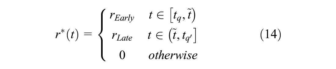
From a behavioral point of view, it is natural to assume that if prevailing patterns do not fully satisfy the equilibrium conditions, all travelers are likely to respond in some way. As a result, the day-to-day dynamics should consider adjustments of departure rates at all time intervals. In addition, simultaneous adjustment of the entire departure rate vector may seem intuitively more efficient computationally. Perhaps these are some of the reasons that caused researchers to examine simultaneous adjustment methods, such as the replicator dynamics ( 8 ) studied by Iryo ( 9 ), the proportional swap system ( 10 ), and the network tatonnement process ( 11 ) studied by Guo et al. ( 5 ). Although these adjustment methods have been proven to converge for other models (e.g., route choice), they exhibit instability in the context of the bottleneck model. The instability of the replicator dynamics, regardless of step size, has been proven mathematically in Iryo ( 9 ), by analysis of a continuous dynamical system that captures the limit when the step size approaches zero. Instabilities of the other two dynamics have been demonstrated numerically ( 5 ). Additional illustrations of unstable dynamics have been presented by Bressan et al. ( 12 ).

Guo et al. (5) proposed bounded rationality as a way of addressing the issue of stability in the bottleneck model. Figure 1 presents a replication of one of their scenarios, with total demand N = 6,000; value of time α = 10 $/h; early arrival penalty of β = $5/h; late arrival penalty of γ = $15/h; and bounded-rationality threshold of ε = $2. The figure includes within-day profiles of departure rates (1a), generalized cost (1b), and convergence (1c). The solution satisfies the conditions of bounded rationality, but it is quite different from the equilibrium solution under perfect rationality, as the threshold is relatively high, ∼36% of the minimum cost. Changing the bounded-rationality threshold from ε = $2 to ε = $1 is not helpful, as the process becomes unstable even with a step size that is 100 times smaller. Therefore, when the bound of rationality is not as wide, the issue of stability is still pertinent.

Figure 1.

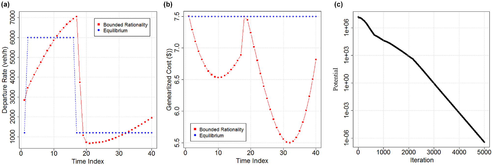
Departure rate and generalized cost profiles under bounded rationality. Replication of a scenario from Guo et al. ( 5 ): (a) within-day departure rates; (b) within-day generalized costs; and (c) convergence of the potential.

Methods

The methods studied in this paper are all variants of the fixed max-to-min shift. To simplify the comparison between these methods, we ignore the potential impact of the initial solution, and assume (unless stated otherwise) that the total number of commuters is initially evenly divided among all intervals, that is, $r_{i}^{0} = r_{0} = \frac{N}{M} \forall 1 \leq i \leq M$ .

For a given shift size, $Δ$ , every max-to-min shift iteration consists of the following steps:

Find the departure time with the maximum travel cost value, $i_{high}^{n} \in argmax (C_{i} (r^{(n)}) : 1 \leq i \leq M)$ . If multiple intervals have the same maximal cost, arbitrarily choose the earliest one.

Find the departure time with the minimum travel cost value, $i_{low}^{n} \in argmin (C_{i} (r^{(n)}) : 1 \leq i \leq M)$ . If multiple intervals have the same minimal cost, arbitrarily choose the earliest one.

Shift $Δ$ (or as much as possible) from the chosen interval with the maximum travel cost value to the chosen interval with the minimum travel cost.

r_{i}^{n + 1} = {\begin{matrix} {[r_{high}^{n} - Δ]}_{+} & i = i_{high}^{n} \\ r_{low}^{n} + \min (Δ, r_{high}^{n}) & i = i_{low}^{n} \\ r_{i}^{n} & otherwise \end{matrix} \forall 1 \leq i \leq M

(16)

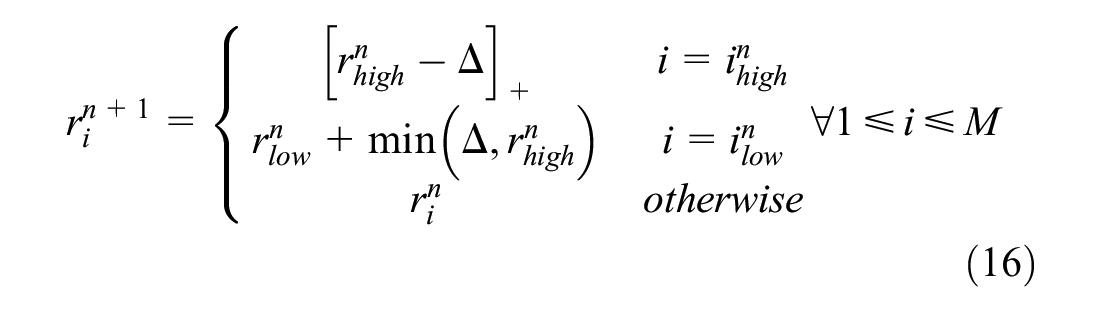
In the basic method we explore shift size that is determined upfront and remains fixed during all iterations. We explore the performance of this basic approach for different values of the fixed shift size. In other adaptive (or semi-adaptive) variants of the max-to-min method, shift size changes along the iterations. Unless stated otherwise, all adaptive methods explored here assume that the initial shift size is equal to the initial departure rate, that is, $Δ_{0} = r_{0} = N / M$ . Shift size can be modified by a pre-specified schedule, for example dividing the shift size by a fixed constant every fixed number of iterations. We explore the performance of this semi-adaptive approach for different combinations of shift reduction frequency and shift reduction factor. Presumably, it may be necessary to adjust these parameters according to the behavior of the specific model under consideration. In that sense this semi-adaptive approach is not likely to be fully generic. In an attempt to identify a generic method, we examined two additional adaptive approaches:

Reducing the shift size value (dividing it by a pre-determined factor) each time the measure value in the current iteration does not decrease compared with the previous one.

Determine the shift size value in each iteration by multiplying the current RMS measure with a pre-determined constant.

Results

In this section we illustrate numerically the performance properties of the max-to-min shift approach, for both fixed shift size and adaptive methods. All examples consider the basic bottleneck model, with a single origin, single destination, single link, homogenous travelers, and deterministic costs. Like Gou et al. ( 5 ), the value of travel time is α = $10/h, the penalty for earliness relative to the desired arrival time is β = $5/h, and the penalty for lateness relative to the desired arrival time is γ = $15/h. The model horizon is 06:00 to 09:00 a.m. (i.e., the length of the simulation is 3 h) and it is discretized into M = 60 time interval (i.e., the length of each interval is Δt = 0.05 h). The preferred arrival time of all commuters is 08:00 a.m. (i.e., t^* = 2 h from the beginning of the simulation).

Additional input parameters for the basic model are the total number of commuters, N, and the capacity of the bottleneck, s. Guo et al. ( 5 ) used N = 6,000 and s = 150, leading to $r_{Early}$ = 300 and $r_{Late}$ = 60. Preliminary experiments showed that when the fixed shift size divides both $r_{Early}$ and $r_{Late}$ , an exact solution can be found in a finite number of iterations. Such results may lead to an over-optimistic impression, reflecting unique conditions that cannot be guaranteed in general. Therefore, in the following experiments we randomly modified these parameters to N = 5,100 and s = 176.68 vehicles per interval.

Fixed Shift Size

We first look at the results of the algorithm where the shift size is fixed and identical in each iteration. For this purpose, seven different fixed shift sizes were selected: 25, 10, 5, 1, 1/2, 1/4, and 1/10. Each shift was tested by running 100,000 iterations. The results expressed as potential as a function of iteration are shown in Figures 2 and 3, while the equivalent results expressed as RMS are shown in Figures 4 and 5.

Figure 2.

The potential measure of convergence as a function of iterations for fixed shift sizes of 1/2, 1/4, and 1/10.

Figure 3.

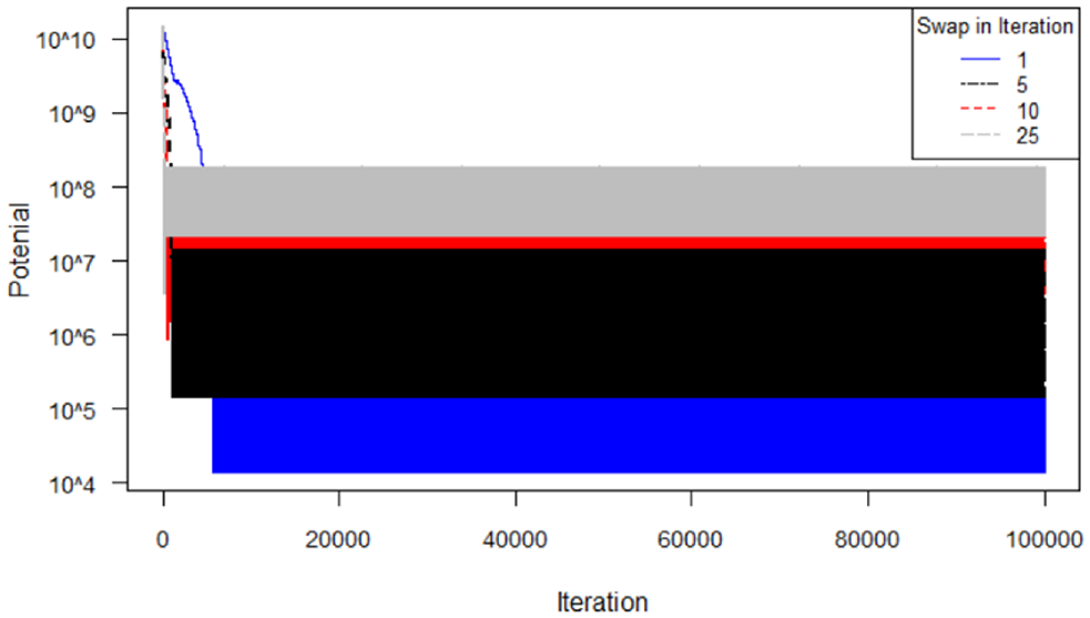
The potential measure of convergence as a function of iterations for fixed shift sizes of 25, 10, 5, and 1.

Figure 4.

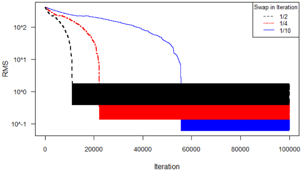
The RMS measure of convergence as a function of iterations for fixed shift sizes of 1/2, 1/4, and 1/10.

Figure 5.

The RMS measure of convergence as a function of iterations for fixed shift sizes of 25, 10, 5, and 1.

The fixed shift size results show that both the potential and the RMS values decrease, at least initially, thereby getting closer to equilibrium. However, after the initial decrease it appears that the measures stabilize within a range of values, which is constant for the remaining iterations. For larger shift sizes, this stabilization in potential and RMS values occurs at a higher range of values, but the initial decrease is faster and, therefore, the method stabilizes earlier compared with smaller shift sizes.

To illustrate the quality of equilibrium approximation obtained by fixed shift size iterations, Figures 6 and 7 present the details of the best approximation solution (lowest RMS) obtained by a fixed shift size of 0.1. In Figure 5 the focus is on commuter departures per interval as a function of departure time, with different symbols for intervals where the cost is practically minimal (up to $10^{- 5}$ ), above minimum but below the RMS, and above the RMS. In Figure 6 the focus is on generalized cost as a function of departure time, with different symbols for intervals with zero departures, intervals where the number of departures is below capacity, and intervals where the number of departures is above capacity. To facilitate the evaluation of this solution, the figures also illustrate the relevant values obtained by Vickrey’s closed form Equations 9 to 15 for $r_{Early}$ , $r_{Late}$ , $t_{q}, \tilde{t}$ , $t_{q'}$ , and C^*.

Figure 6.

Commuter departures as a function of departure time for the best approximation solution (minimum RMS value) obtained by fixed shifts of size 0.1.

Figure 7.

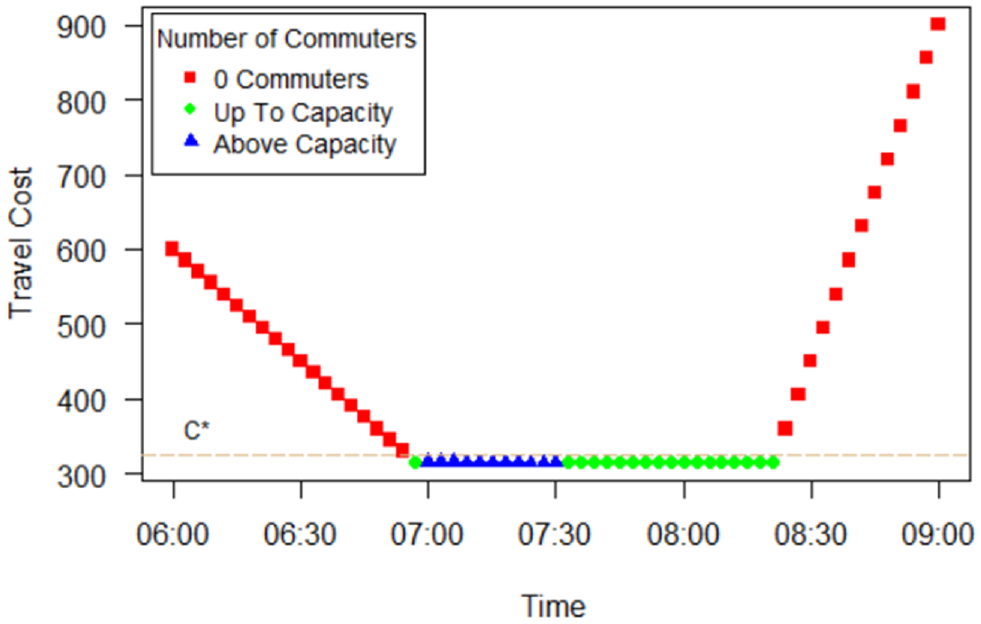
Generalized cost as a function of departure time for the best approximation solution (lowest RMS) obtained by fixed shifts of size 0.1.

Figures 6 and 7 show that this solution is indeed a reasonable approximation of the equilibrium solution. During the intervals in [ $t_{q}, t_{q'}]$ the generalized cost is very close to the equilibrium cost, while at other intervals there are no departures. Furthermore, during [ $t_{q}, \tilde{t})$ commuter departures are fairly close to $r_{Early}$ and during ( $\tilde{t}, t_{q'}]$ commuter departures are fairly close to $r_{Late}$ . The two exceptions are the interval at $t_{q}$ and the interval at $\tilde{t}$ . These exceptions are related to the discretization of the solution. The amount of commuter departures at the interval containing $\tilde{t}$ is a weighted average of $r_{Early}$ and $r_{Late}$ , while the deviation at $t_{q}$ is associated with the non-uniqueness of the discretized equilibrium, as explained by Ramadurai et al. ( 4 ).

Figure 8 shows the lowest RMS and potential values over all iterations, for every given shift size. The minimum RMS value is approximately proportional to the step size, while the minimum potential value is approximately quadratic in step size. These results suggest that any desired precision of approximation of the equilibrium solution may be attained by choosing a sufficiently small step size. Yet the number of iterations may increase as well, and thus the fixed shift approach is probably not the most effective option. Other variants of this method, semi-adaptive and adaptive, will be further explored below.

Figure 8.

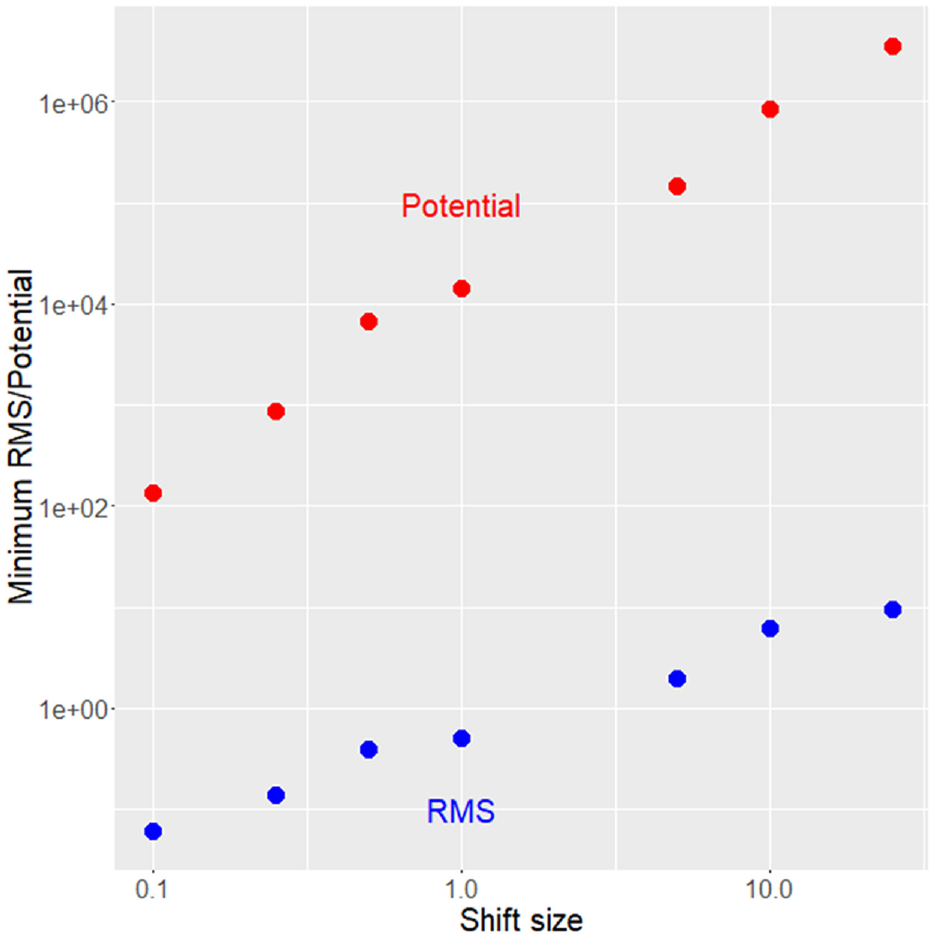
Minimum potential and RMS over all iterations, as function of fixed shift size.

Adaptive Shift Size

Figures 9 and 10 show the potential and RMS for the semi-adaptive approaches when the shift size is divided by 5 every 50, 300, 750, and 1,500 iterations. Among these options, the best convergence is achieved when shift size is divided by 5 every 300 iterations, reaching the limits of machine precision after less than 8,000 iterations. When shift size is divided every 750 or 1,500 iterations, convergence is stable but slower. However, dividing shift size by 5 every 50 iterations lead to a lack of convergence, as the shift size becomes too small too soon to enable convergence to equilibrium.

Figure 9.

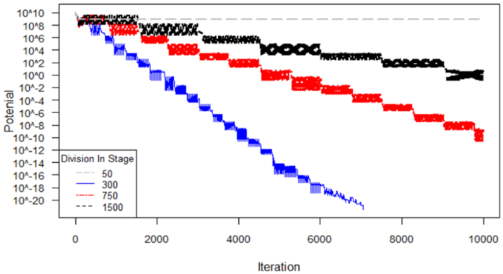
Potential of the system for 10,000 iterations, dividing shift size by 5 every 50, 300, 750, and 1,500 iterations.

Figure 10.

RMS of the system for 10,000 iterations, dividing shift size by 5 every 50, 300, 750, and 1,500 iterations.

Figures 11 and 12 show the potential and RMS for the semi-adaptive approaches when the shift size is divided by 2, 5, 10, and 20 every 300 iterations. In this case division by 20 does not lead to convergence, for a similar reason as dividing shift size by 5 every 50 iterations, but all other options are leading to convergence.

Figure 11.

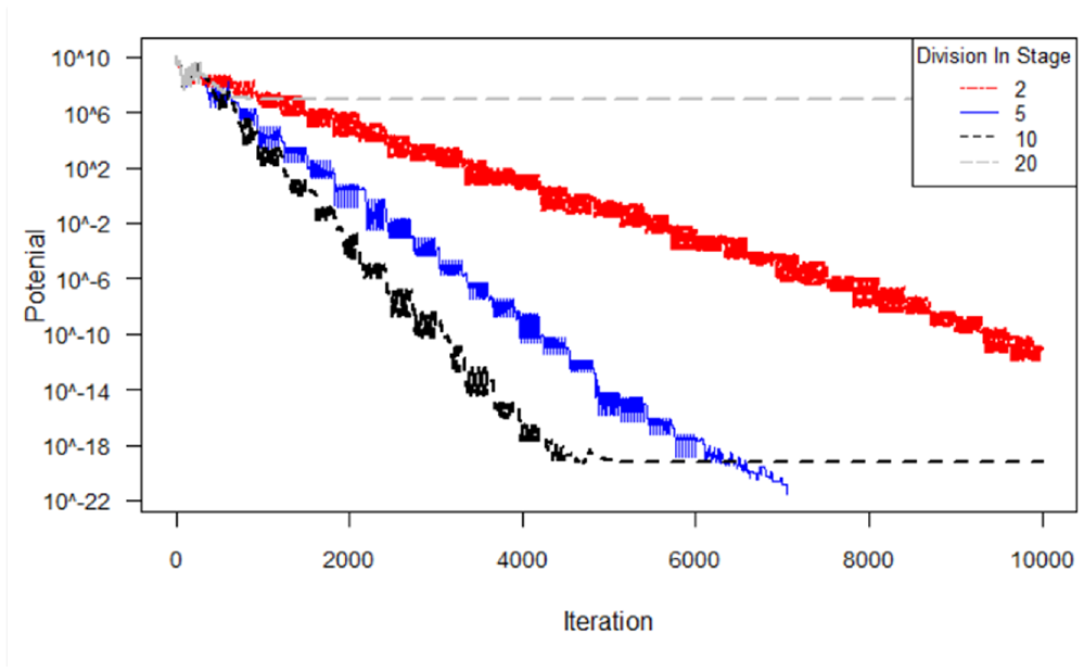
Potential of the system for 10,000 iterations, dividing shift size by 2, 5, 10, and 20 every 300 iterations.

Figure 12.

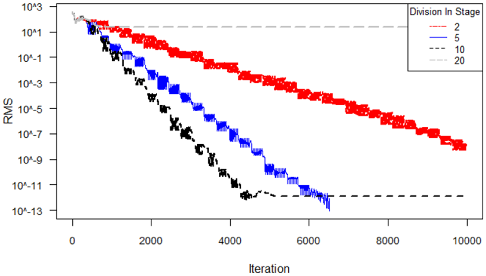
RMS of the system for 10,000 iterations, dividing shift size by 2, 5, 10, and 20 every 300 iterations.

Figures 13 and 14 show results for an adaptive approach where shift size is reduced each time the measure value in the current iteration does not decrease compared with the previous one. This approach seems to be particularly sensitive to the division factor, where a factor of 1.05 leads to convergence, while a slightly higher factor of 1.3 (or larger) is too big and does not lead to convergence. Finally, Figures 15 and 16 show results for an adaptive approach where shift size is determined by multiplying the current RMS measure with a pre-determined constant. In this case, using a constant value of 1/2 results in convergence after about 2,000 iterations, while a constant value of 1/5 results in slightly slower convergence, after about 4,000 iterations. On the other hand, a constant of 1 or higher leads to lack of convergence.

Figure 13.

Potential of the system for 10,000 iterations dividing shift size by 1.05, 1.3, 1.5, and 1.8 each time the potential in the current iteration does not decrease compared with the previous.

Figure 14.

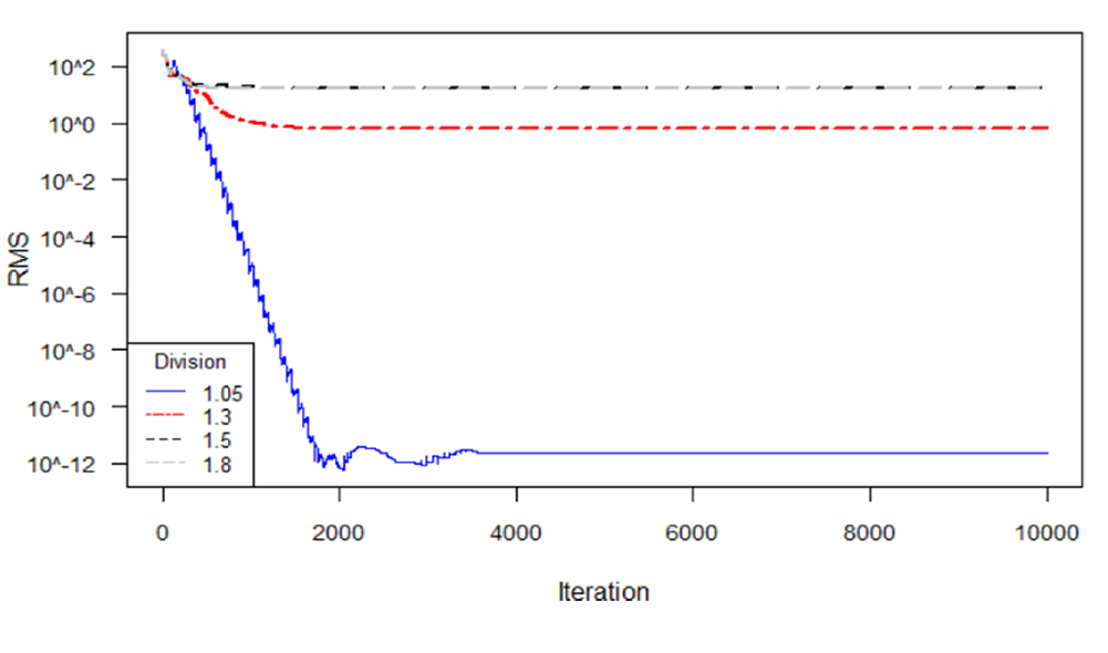
RMS of the system for 10,000 iterations dividing shift size by 1.05, 1.3, 1.5, and 1.8 each time the potential in the current iteration does not decrease compared with the previous.

Figure 15.

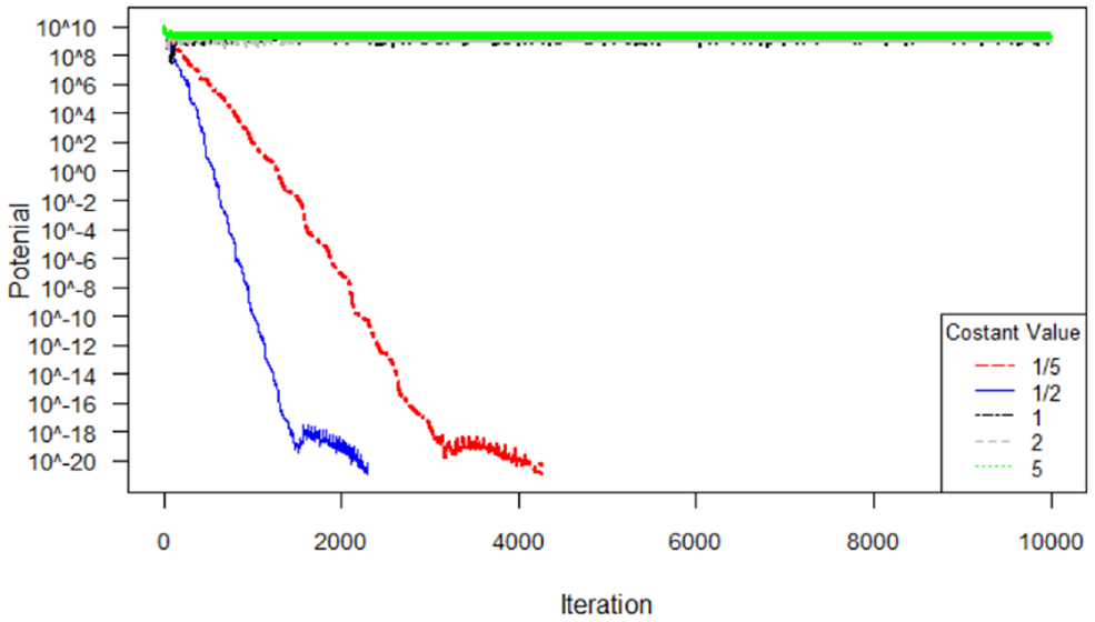
Potential of the system for 10,000 iterations, determining the shift size value in each iteration by the current RMS measure, multiplied by 0.2, 0.5, 1, 2, and 5.

Figure 16.

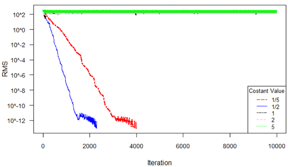
RMS of the system for 10,000 iterations, determining the shift size value in each iteration by the current RMS measure, multiplied by 0.2, 0.5, 1, 2, and 5.

In summary, the simple principle of making one shift per iteration, from the maximum cost interval to the lowest cost interval, seems to be a good basis for achieving numerical convergence. Setting the shift amount requires some tuning. If multiple instances of a similar model are solved, a specific shift value may be identified for one instance, and it can be expected that the same value will provide useful results in other similar instances as well. Using a semi-adaptive approach, tuned for a specific instance, can be expected to work well for an even wider range of similar instances. However, developing a fully adaptive method that can effectively address all model instances seems to be a bigger challenge, yet to be resolved.

Conclusions

Identifying generic methods for departure time choice models is a challenge that so far has not been resolved by existing literature. The lack of such methods is problematic practically, especially when numerical solutions are sought for complex models in which departure time choice is embedded, since in such models analytic closed form solutions are often difficult to obtain. In addition, a theoretical concern has been raised since equilibrium is conceivably a reasonable representation of reality only if it can be associated with stable dynamics.

Our results show that a simplistic method of shifting travelers from the travel time interval with highest cost to the interval with lowest cost can lead to a convergent process for the basic departure time choice model. If the shift size is fixed, then the process stabilizes within a set of solutions whose deviation from equilibrium (in RMS) is proportional to the pre-determined shift size. If the shift size is adaptive, for example a properly chosen constant multiplied by the RMS value, then convergence to machine precision is observed.

Future research should examine the sensitivity of the parameters of the method to instance inputs, and whether similar methods can be used for heterogenous models, stochastic models, or both. It would be desirable for the numerical findings presented here to be supported by a mathematical theory, including a proof of convergence. Finally, other converging methods should be sought, to improve convergence speed, the representation of realistic dynamics, or both.

Footnotes

Author Contributions

The authors confirm contribution to the paper as follows: study conception and design: A. Daly and H. Bar-Gera; analysis and interpretation of results: A. Daly and H. Bar-Gera; draft manuscript preparation: A. Daly and H. Bar-Gera. All authors reviewed the results and approved the final version of the manuscript.

Declaration of Conflicting Interests

The author(s) declared no potential conflicts of interest with respect to the research, authorship, and/or publication of this article.

Funding

The author(s) received no financial support for the research, authorship, and/or publication of this article.

References

Vickrey

W. S.

Congestion Theory and Transport Investment. The American Economic Review, Vol. 59, No. 2, 1969, pp. 251–260.

Small

K. A.

The Bottleneck Model: An Assessment and Interpretation. Economics of Transportation, Vol. 4, No. 1–2, 2015, pp. 110–117.

Lindsey

Existence, Uniqueness, and Trip Cost Function Properties of User Equilibrium in the Bottleneck Model with Multiple User Classes. Transportation Science, Vol. 38, No. 3, 2004, pp. 293–314.

Ramadurai

Ukkusuri

S. V.

Zhao

Pang

Linear Complementarity Formulation for Single Bottleneck Model with Heterogeneous Commuters. Transportation Research Part B: Methodological, Vol. 44, No. 2, 2010, pp. 193–214.

Guo

R. Y.

Yang

Huang

H. J.

Day-to-Day Departure Time Choice under Bounded Rationality in the Bottleneck Model. Transportation Research Part B: Methodological, 2017. (In press). https://doi.org/10.1016/j.trb.2017.08.016.

Van Leeuwen

van de Ven

P. M.

Modelling User Behaviour at a Stochastic Road Traffic Bottleneck. Proc., 11th EAI International Conference on Performance Evaluation Methodologies and Tools, Venice, Italy, 2017. https://doi.org/10.1145/3150928.3150933.

Jin

W. L.

Stable Day-to-Day Dynamics for Departure Time Choice. Transportation Science, Vol. 54, No. 1, 2020, pp. 42–61. https://doi.org/10.1287/trsc.2019.0919.

Schuster

Sigmund

Replicator Dynamics. Journal of Theoretical Biology, Vol. 100, 1983, pp. 533–538.

Iryo

Instability of Departure Time Choice Problem: A Case with Replicator Dynamics. Transportation Research Part B: Methodological, Vol. 126, 2019, pp. 353–364.

10.

Smith

M. J.

The Stability of a Dynamic Model of Traffic Assignment - An Application of a Method of Lyapunov. Transportation Science, Vol. 18, No. 3, 1984, pp. 245–252.

11.

Friesz

T. L.

Bernstein

Mehta

N. J.

Tobin

R. L.

Ganjalizadeh

Day-to-Day Dynamic Network Disequilibrium and Idealized Traveler Information Systems. Operations Research, Vol. 42, No. 6, 1994, pp. 1120–1136.

12.

Bressan

Liu

C. J.

Shen

Variational Analysis of Nash Equilibria for a Model of Traffic Flow. Quarterly Applied Mathematics, Vol. 70, No. 3, 2012, pp. 495–515.