Empirical Estimation of Shortest Route Length along U.S. Interstate Highways Based on Great Circle Distance

Abstract

In this study, 98 regression models were specified for easily estimating shortest distances based on great circle distances along the U.S. interstate highways nationwide and for each of the continental 48 states. This allows transportation professionals to quickly generate distance, or even distance matrix, without expending significant efforts on complicated shortest path calculations. For simple usage by all professionals, all models are present in the simple linear regression form. Only one explanatory variable, the great circle distance, is considered to calculate the route distance. For each geographic scope (i.e., the national or one of the states), two different models were considered, with and without the intercept. Based on the adjusted R-squared, it was observed that models without intercepts generally have better fitness. All these models generally have good fitness with the linear regression relationship between the great circle distance and route distance. At the state level, significant variations in the slope coefficients between the state-level models were also observed. Furthermore, a preliminary analysis of the effect of highway density on this variation was conducted.

Calculating route distances along transportation networks is a classical and well-established procedure in transportation fields. Route distances are usually estimated using classic shortest paths algorithms including, but not limited to, Dijkstra’s algorithm, the Bellman–Ford algorithm, the Floyd–Warshall algorithm, and so on. Open-source codes of these algorithms are publicly available, and they are also usually included in commercial software (e.g., ArcGIS pro). Accessing these tools is typically not an issue for well-trained transportation engineers who are experienced in network modeling and analysis. However, this still requires noticeable efforts. In addition to the ability to use the right tool or algorithm, transportation engineers are usually required to establish the transportation network represented either in graph or GIS shapefiles for different network scopes. Corrections and adjustments are also inevitable if high-quality transportation network data are not available. In addition, route distance calculation could cause computational challenges if both the network size and the number of origin–destination (O-D) pairs required for route distance calculations are large. These challenges create obstacles for many transportation projects, especially project teams that have limited access to or do not have sufficient training to use these tools and/or if calculating exact route distances is not the primary focus.

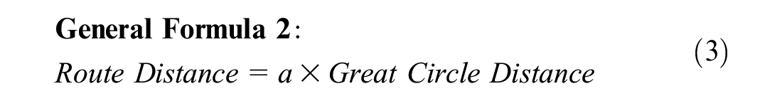
An alternative method is to use statistical regression models to estimate the route distance using the great circle distance between any two O-D pairs with their geographic coordinates. An example of a previous application is the usage of the simple linear regression model based on the intra-city New York City (NYC) data to evaluate the feasibility of battery electric vehicles in taxi fleets in the city of New York ( 1 , 2 ). The NYC model is shown in Equation 1 (distances are measured in miles), and its slope coefficient (also known as circuity) is 1.4413, close to the square root of 2, which reflects the taxicab geometry pattern of the roadway networks in NYC ( 1 , 3 ). With a sample of 51 Metropolitan Statistical Areas (MSAs), another study evaluated the historical trends in the changing slope coefficient with recent street network expansion ( 4 ). In addition to passenger vehicle route distance estimation, there is also a prior application for freight shipment, and a slope of 1.22 was suggested to estimate freight route distances using the great circle distances ( 5 ). All of these prior regression models are mode-, scope-, and geography specific, and therefore cannot be simply generalized to other scopes.

\begin{matrix} NYC Model : Route Distance \\ = 1.441 \times Euclidean Distance + 0.138 \end{matrix}

(1)

There is no database available in the literature for this type of regression model for estimation of the inter-city passenger vehicle trip distance. Therefore, in this study, the aim is to develop a database that contains regression models to estimate the route distance for passenger vehicles along U.S. interstate highways at both national and individual state geographic scopes. For simplicity, by using models for a general audience, similar to the model reported by Zhan et al., the reported regression models are in the form of simple linear regression models using only the great circle distance as the explanatory variable to estimate the route distance ( 1 ).

Data and Methods

To generate the empirical regression models to estimate the route distance at both U.S. national and state-level scopes, the U.S. mainland interstate highway network was used in the analysis, as shown in Figure 1. The interstate highway network was preprocessed into a network graph in our previously reported study ( 6 ). Along the graph, the interstate highway network is represented using the undirected graph G(N, A), in which N represents nodes and A represents undirected arcs symmetrically connecting these nodes. To represent the U.S. mainland interstate highway network, 4,300 nodes are present in the graph, connected with 10,666 undirected arcs. The median arc length is 10.23 mi and the maximum length is 29.6 mi.

Figure 1.

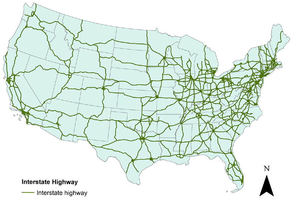
U.S. mainland interstate highway network.

The empirical statistical models on the route distance are fitted by random sampling of O-D pairs between 4,300 nodes. The great circle distance is estimated based on coordinates of both the origin and destination nodes for each O-D pair. The coordinates are determined based on this geographic location using the ArcGIS software. The route distance between each O-D pair is calculated using Dijkstra’s algorithm along the graph with the open-source C++ code ( 7 ). Simple linear regression is conducted to fit the regression models. The general formula I is shown in Equation 2. In Equation 2, a is the slope coefficient, and b (unit: miles) is the intercept. As an alternative to the general formula in 2, another regression model is also fitted without the intercept, as shown in Equation 3. All distances are measured in miles.

\begin{matrix} General Formula 1 : \\ Route Distance = a \times Great Circle Distance + b \end{matrix}

(2)

\begin{matrix} General Formula 2 : \\ Route Distance = a \times Great Circle Distance \end{matrix}

(3)

The models were developed for the national scale with 10,000 sampled O-D pairs, and models for all U.S. mainland states with a maximum 500 sampled O-D pairs for each state-level model. All regression analyses are conducted using R.

Results

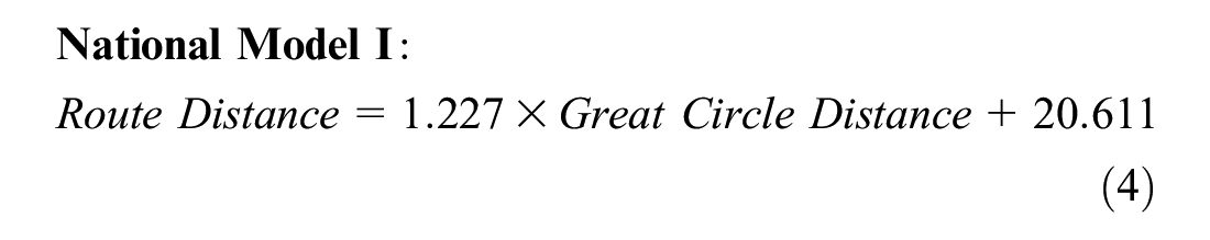
With 10,000 sampled O-D pairs at the national scale, Equation 4 shows the fitted empirical model, the National Model I, to estimate the route distance along U.S. interstate highways at the U.S. national scope. The model has good fitness over the 10,000 sampled distance data and has an adjusted R-squared value of 0.983. It is noted that the slope coefficient is 1.227 lower than the value of 1.441 obtained for the NYC model ( 1 ). This is because interstate highways have a reduced taxicab geometry pattern compared to the NYC roadways and the actual route distance is closer to the great circle distance.

The National Model I in Equation 4 is limited as it can yield unexpected results, especially when the great circle distance is relatively small. For example, when the great circle distance is close to 0, the route distance should also be close to 0. However, with the intercept, the model yields a route distance of 20.611 mi. To overcome this issue, the regression model was also fitted without the intercept, and the new National Model II is shown in Equation 5. Compared to Equation 4, this new model has a slightly higher slope coefficient, and has a higher adjusted R-square of 0.995. The results indicate that a potential better fitness of the regression model is obtained without the intercept for estimating the route distance.

\begin{matrix} National Model I : \\ Route Distance = 1.227 \times Great Circle Distance + 20.611 \end{matrix}

(4)

\begin{matrix} National Model II : \\ Route Distance = 1.242 \times Great Circle Distance \end{matrix}

(5)

In addition to the national models in Equations 4 and 5 that could be used generally for any O-D pairs along the U.S. mainland interstate highways, we also fitted state-level empirical statistical models, namely State-Level Model I, to estimate O-D route distance within each state. Table 1 shows summaries of the linear regression models with intercepts for all 48 mainland states with key regression statistics of coefficients, t-values, p-values, and adjusted R-squares. All these models generally have good fitness with the linear regression relationship between the great circle distance and route distance, with the lowest R-square at 45.6%. All slope coefficients are significant, with p-values smaller than 0.001 for all states. The intercept coefficients are significant for some states (e.g., p-value: <0.001 for California [CA]), and are not significant for other states (e.g., p-value: 0.174 for Texas [TX]).

Table 1.

Statistics of State-Level Model I (with Intercepts)

State	Coefficient		t-Value		p-Value		Adjusted R-square (%)
State	Slope	Intercept	Slope	Intercept	Slope	Intercept	Adjusted R-square (%)
AL	1.22	12.69	53.36	4.28	<0.001	<0.001	85.1
AR	1.30	−2.89	79.42	−1.50	<0.001	0.133	92.7
AZ	1.78	−9.24	42.97	−1.57	<0.001	0.118	78.8
CA	1.30	10.57	191.43	5.42	<0.001	<0.001	98.7
CO	1.36	0.81	67.55	0.31	<0.001	0.757	90.2
CT	1.19	4.07	69.33	6.13	<0.001	<0.001	90.6
DE	1.08	0.82	114.57	1.98	<0.001	0.052	99.5
FL	1.15	8.93	109.38	4.37	<0.001	<0.001	96.0
GA	1.25	6.15	54.93	1.92	<0.001	0.055	85.8
IA	1.20	7.99	77.70	3.75	<0.001	<0.001	92.4
ID	1.70	−28.32	63.10	−5.24	<0.001	<0.001	89.0
IL	1.18	10.94	95.22	5.92	<0.001	<0.001	94.8
IN	1.17	12.88	72.70	6.28	<0.001	<0.001	91.4
KS	1.15	8.48	91.84	4.59	<0.001	<0.001	94.4
KY	1.17	12.02	96.18	6.64	<0.001	<0.001	94.9
LA	1.35	1.63	57.92	0.48	<0.001	0.633	87.1
MA	1.20	2.05	121.95	3.64	<0.001	<0.001	96.8
MD	1.24	2.26	94.96	3.06	<0.001	0.002	94.8
ME	1.19	−1.17	220.74	−1.92	<0.001	0.056	99.5
MI	1.16	8.99	66.78	4.56	<0.001	<0.001	90.0
MN	1.23	1.27	94.34	0.93	<0.001	0.352	94.7
MO	1.30	18.27	35.71	2.96	<0.001	0.003	71.9
MS	1.40	4.61	62.44	1.61	<0.001	0.107	88.7
MT	1.39	18.39	54.86	3.52	<0.001	<0.001	85.8
NC	1.14	14.78	70.84	7.07	<0.001	<0.001	91.0
ND	1.28	−6.82	60.94	−1.93	<0.001	0.054	92.0
NE	1.14	−1.87	95.96	−0.79	<0.001	0.431	96.9
NH	1.12	4.05	33.23	2.60	<0.001	0.010	86.7
NJ	1.14	3.58	104.68	5.32	<0.001	<0.001	95.7
NM	1.48	4.60	54.28	0.95	<0.001	0.342	85.5
NV	2.49	−96.07	64.98	−10.32	<0.001	<0.001	92.4
NY	1.34	−0.63	134.14	−0.38	<0.001	0.702	97.3
OH	1.16	9.17	94.37	5.82	<0.001	<0.001	94.7
OK	1.18	6.96	69.53	3.73	<0.001	<0.001	90.7
OR	1.68	−32.07	90.54	−9.66	<0.001	<0.001	94.3
PA	1.24	9.21	94.05	4.50	<0.001	<0.001	94.7
RI	1.31	−0.07	50.70	−0.16	<0.001	0.875	90.4
SC	1.11	10.57	70.63	6.65	<0.001	<0.001	90.9
SD	1.26	−6.15	86.05	−2.13	<0.001	0.033	93.7
TN	1.22	2.89	111.82	1.64	<0.001	0.102	96.2
TX	1.27	7.67	64.61	1.36	<0.001	0.174	89.3
UT	1.62	1.74	40.44	0.31	<0.001	0.760	76.7
VA	1.31	0.18	115.99	0.11	<0.001	0.913	96.4
VT	1.20	24.14	13.84	4.25	<0.001	<0.001	45.6
WA	1.53	0.25	74.54	0.10	<0.001	0.924	91.8
WI	1.30	21.43	33.86	3.89	<0.001	<0.001	69.7
WV	1.48	1.00	65.04	0.48	<0.001	0.632	89.5
WY	2.03	−28.88	38.55	−3.13	<0.001	0.002	74.9

Note: AL = Alabama; AZ = Arizona; AR = Arkansas; CA = California; CO = Colorado; CT = Connecticut; DE = Delaware; FL = Florida; GA = Georgia; ID = Idaho; IL = Illinois; IN = Indiana; IA = Iowa; KS = Kansas; KY = Kentucky; LA = Louisiana; ME = Maine; MD = Maryland; MA = Massachusetts; MI = Michigan; MN = Minnesota; MS = Mississippi; MO = Missouri; MT = Montana; NE = Nebraska; NV = Nevada; NH = New Hampshire; NJ = New Jersey; NM = New Mexico; NY = New York; NC = North Carolina; ND = North Dakota; OH = Ohio; OK = Oklahoma; OR = Oregon; PA = Pennsylvania; RI = Rhode Island; SC = South Carolina; SD = South Dakota; TN = Tennessee; TX = Texas; UT = Utah; VT = Vermont; VA = Virginia; WA = Washington; WV = West Virginia; WI = Wisconsin; WY = Wyoming.

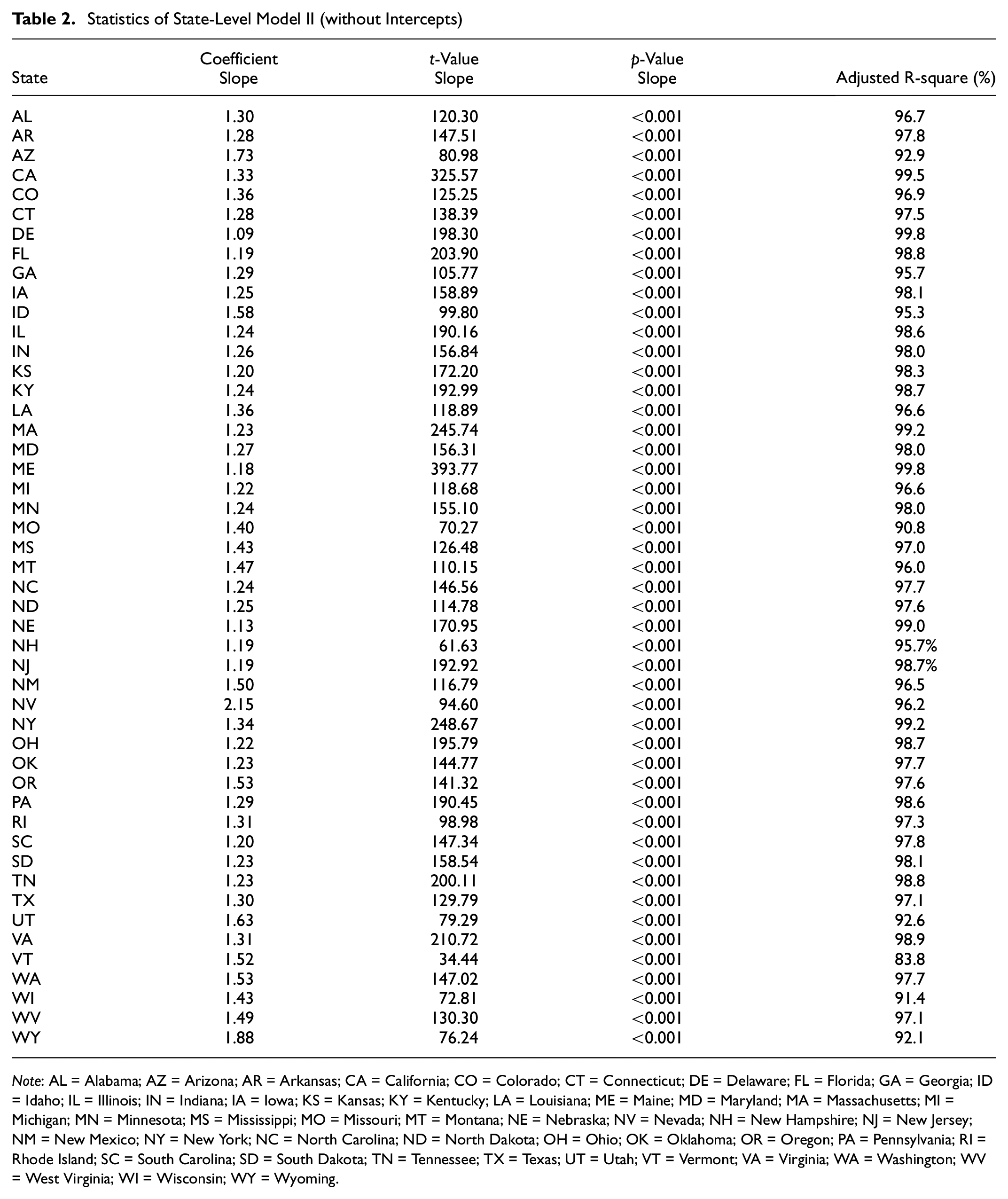
Similar to the National Model II, we also fitted state-level models without intercepts, namely State-Level Model II, with key regression statistics as shown in Table 2. Compared to Tables 1, 2 does not contain any statistics of the intercept, which is excluded in the model. All slope coefficients have a significant fitness for all states with p-values < 0.001. For the state-level, Model II has higher adjusted R-squares compared to the Model I for all states. Combined with the national level results, it indicates that the presence of intercepts normally does not improve the fitness of the route distance regression models. However, there is no conclusion as to which model to choose, as the decision is highly dependent on additional considerations by different users.

Table 2.

Statistics of State-Level Model II (without Intercepts)

State	Coefficient	t-Value	p-Value	Adjusted R-square (%)
State	Slope	Slope	Slope	Adjusted R-square (%)
AL	1.30	120.30	<0.001	96.7
AR	1.28	147.51	<0.001	97.8
AZ	1.73	80.98	<0.001	92.9
CA	1.33	325.57	<0.001	99.5
CO	1.36	125.25	<0.001	96.9
CT	1.28	138.39	<0.001	97.5
DE	1.09	198.30	<0.001	99.8
FL	1.19	203.90	<0.001	98.8
GA	1.29	105.77	<0.001	95.7
IA	1.25	158.89	<0.001	98.1
ID	1.58	99.80	<0.001	95.3
IL	1.24	190.16	<0.001	98.6
IN	1.26	156.84	<0.001	98.0
KS	1.20	172.20	<0.001	98.3
KY	1.24	192.99	<0.001	98.7
LA	1.36	118.89	<0.001	96.6
MA	1.23	245.74	<0.001	99.2
MD	1.27	156.31	<0.001	98.0
ME	1.18	393.77	<0.001	99.8
MI	1.22	118.68	<0.001	96.6
MN	1.24	155.10	<0.001	98.0
MO	1.40	70.27	<0.001	90.8
MS	1.43	126.48	<0.001	97.0
MT	1.47	110.15	<0.001	96.0
NC	1.24	146.56	<0.001	97.7
ND	1.25	114.78	<0.001	97.6
NE	1.13	170.95	<0.001	99.0
NH	1.19	61.63	<0.001	95.7%
NJ	1.19	192.92	<0.001	98.7%
NM	1.50	116.79	<0.001	96.5
NV	2.15	94.60	<0.001	96.2
NY	1.34	248.67	<0.001	99.2
OH	1.22	195.79	<0.001	98.7
OK	1.23	144.77	<0.001	97.7
OR	1.53	141.32	<0.001	97.6
PA	1.29	190.45	<0.001	98.6
RI	1.31	98.98	<0.001	97.3
SC	1.20	147.34	<0.001	97.8
SD	1.23	158.54	<0.001	98.1
TN	1.23	200.11	<0.001	98.8
TX	1.30	129.79	<0.001	97.1
UT	1.63	79.29	<0.001	92.6
VA	1.31	210.72	<0.001	98.9
VT	1.52	34.44	<0.001	83.8
WA	1.53	147.02	<0.001	97.7
WI	1.43	72.81	<0.001	91.4
WV	1.49	130.30	<0.001	97.1
WY	1.88	76.24	<0.001	92.1

With all slope coefficients being significant, huge variations are observed between states and slopes for both Model I and Model II. For example, for Model I, it could range between 1.08 and 2.49. Figure 2 shows the geographic variations on the slope coefficient with the intercept. It is shown that the slope coefficients are generally higher in the west region of the U.S. compared to the other parts of the country. This indicates the same great circle distance measured between any O-D pair could result in much longer route distance in this region.

Figure 2.

Geographic variations of the slope coefficient in the state-level empirical statistical models of route distance estimation.

Many potential factors could contribute to this variation in the slope coefficients at different states, including, but not limited to, highway distribution patterns, highway density, highway curvatures, and so forth. Many of these factors are difficult to measure and aggregate at state levels. An extensive evaluation of these factors’ effects is beyond the scope of this study and will be considered in future work. This paper only evaluates the effect of one factor, the highway density, on the actual slope coefficients. Compared to other factors, the highway density (unit: miles/100-square miles) is relatively easy to measure, and in this study, can be estimated using Equation 6.

Highway density = \frac{Total length of interstate highways}{Total area of the state}

(6)

Figure 3 shows scatterplots of the slope coefficients for State-Level Model I (with intercept) and interstate highway densities for all mainland states. It is shown that when the highway density is relatively higher (e.g., >4 mi/100-square miles), the variation of slope coefficients is relatively smaller, and the actual slope remains consistently low at the 1.1–1.4 level. The reason is that higher density results in better highway coverage and the route between most O-D pairs tends to take straight lines. On the other hand, if the highway density is relatively low, significant variation is observed in the slope coefficients between states. In this case, the actual O-D route distance heavily depends on other factors, such as the actual distribution patterns of the interstate highway systems as well as their connectivity. An investigation of the effects of other factors will be considered in future work.

Figure 3.

Scatterplots of slope coefficients (with intercept) and interstate highway densities for 48 mainland states.

Conclusion

In this study, a set of empirical regression models was developed to estimate route distances between O-D pairs along interstate highways. Both national-level and state-level models were developed. These models provide an easy-to-use database that allows transportation professionals to quickly estimate route distances for different transportation projects. These models were developed using the simple linear regression model, and only consider one explanatory variable, the great circle distance which is easier to determine based on the coordinates of any origin and destination. For each geographic scope (i.e., national or one of the states), two different models were considered, with and without the intercept. Based on the adjusted R-squared value, it was observed that models without intercepts generally have a better fitness. We also provided preliminary evaluations of the variations in regression coefficients between different state-level models. We found that the highway density is a key factor that contributes to this variation.

For simplicity, this study only considers the interstate highway network, and the empirical statistical models could only estimate route distances along the interstate highways. In reality, other roadway systems (i.e., state, county, and city highways) should also be considered to fully evaluate the route distance between any O-D pair in the U.S. However, this will require additional network preparation in the graph form and larger network systems could result in additional computational efforts. Extending the current scope to all highway systems will be considered in future work.

Footnotes

Author Contributions

The authors confirm contribution to the paper as follows: study conception and design: Z. Lin, F. Xie; data collection: N. Liu, F. Xie; analysis and interpretation of results: N. Liu, F. Xie, Z., Lin, M. Jin; draft manuscript preparation: N. Liu, F. Xie, Z., Lin. All authors reviewed the results and approved the final version of the manuscript.

Declaration of Conflicting Interests

The author(s) declared no potential conflicts of interest with respect to the research, authorship, and/or publication of this article.

Funding

The author(s) disclosed receipt of the following financial support for the research, authorship, and/or publication of this article: This research was supported by the DOE Office of Energy Efficiency and Renewable Energy, Vehicle Technologies Office (Analysis Program). This manuscript has been authored by UT-Battelle, LLC under Contract No. DE-AC05-00OR22725 with the U.S. Department of Energy. The United States Government retains and the publisher, by accepting the article for publication, acknowledges that the United States Government retains a non-exclusive, paid-up, irrevocable, world-wide license to publish or reproduce the published form of this manuscript, or allow others to do so, for United States Government purposes. The Department of Energy will provide public access to these results of federally sponsored research in accordance with the DOE Public Access Plan ().

Data Accessibility Statements

All data generated during this study are included in this published article. All input data analyzed during the current study are available from the corresponding author on reasonable request or from TEEM.ornl.gov.

References

Zhan

Qian

Ukkusuri

S. V.

A Graph-Based Approach to Measuring the Efficiency of an Urban Taxi Service System. IEEE Transactions ono Intelligent Transportation Systems, Vol. 17, No. 9, 2016, pp. 2479–2489.

Dong

Lin

Yang

Analyzing Battery Electric Vehicle Feasibility from Taxi Travel Patterns: The Case Study of New York City, USA. Transportation Research Part C: Emerging Technologies, Vol. 87, 2018, pp. 91–104.

Krause

E. F.

Taxicab Geometry. The Mathematics Teacher, Vol. 66, No. 8, 1973, pp. 695–706.

Giacomin

D. J.

Levinson

D. M.

Road Network Circuity in Metropolitan Areas. Environment and Planning B: Planning and Design, Vol. 42, No. 6, 2015, pp. 1040–1053.

Qureshi

M. A.

Hwang

H.-L.

Chin

S.-M.

Comparison of Distance Estimates for Commodity Flow Survey: Great Circle Distances versus Network-Based Distances. Transportation Research Record: Journal of the Transportation Research Board, 2002. 1804: 212–216.

Liu

Xie

Lin

Jin

Evaluating National Hydrogen Refueling Infrastructure Requirement and Economic Competitiveness of Fuel Cell Electric Long-Haul Trucks. Mitigation and Adaptation Strategies for Global Change, Vol. 25, 2019, pp. 1–17.

Pascoal

Martins

An Implementation of K-Shortest Path Algorithm (Cpp Version). 2020. https://github.com/yan-qi/k-shortest-paths-cpp-version.