



Abstract
Car-following is considered as one of the most prevalent fundamental driving behaviors that substantially influences traffic performance as well as road safety and capacity. Drivers’ car-following behavior is affected by numerous factors. However, in practice, very few of these factors have been scrutinized, because of their latent essence and unavailability of appropriate data. Owing to its importance, drivers’ reaction time has attracted the attention of many researchers; nevertheless, it is considered as a fixed parameter in car-following models, which is far from reality. To take the variability of drivers’ reaction time into account, a flexible hybrid approach has been suggested in the present study. In the proposed structure, in the first step, the desirable acceleration of the driver is estimated by applying an equation-based car-following model. In the next step, the driver’s reaction delay in applying the calculated acceleration is estimated by an artificial neural network. The corresponding parameters are jointly estimated by applying an estimated distribution algorithm. Statistical tests indicate better performance of the hybrid model, which considers the variations of the driver’s reaction time, compared with a traditional model with fixed reaction time. Furthermore, the cross-validation results indicate better generalizability and transferability of the proposed model in action.
Car-following models, as one of the most essential parts of traffic microsimulation tools, have been studied for more than six decades. A car-following model describes the longitudinal motion of vehicles in a lane and explains how a follower vehicle interacts with its leader/leaders in the same lane. Because of the complex and non-linear nature of car-following behavior, a broad range of techniques has been applied by researchers in different fields to model this phenomenon. In general, car-following models can be categorized into two main classes: equation-based car-following models (EBCFM) and data-driven car-following models (DDCFM). In EBCFMs, the process of car-following is described based on differential-algebraic equations, and an explicit mathematical relationship is considered between the input and output variables ( 1 , 2 ). On the other hand, the process of modeling in DDCFMs is mainly conducted by employing computational intelligence and machine learning algorithms (Statistical Learning models), particularly artificial neural network and fuzzy rules ( 3 – 5 ). The ability of artificial neural networks to model complex and non-linear relationships ( 6 ), their independence from prior knowledge and from making any explicit assumption about the type of relationship between the input and output variables, as well as being robust to noise ( 7 ), have turned such models into powerful tools for modeling purposes.
Car-following behavior is a non-linear, complex phenomenon and is affected by several factors. Accordingly, selecting appropriate variables is a crucial step in constructing any car-following model. Although a broad range of variables has been distinguished as the influencing factors on car-following behavior ( 2 ), the driver’s reaction time can be considered as one of the most critical variables and has been incorporated into a broad range of car-following models. Because of its importance, reaction time has been studied in various fields, and different definitions exist for it in the literature ( 8 , 9 ). However, in the traffic flow theory area, which is the context of this study, reaction time is defined as the time taken by the follower in responding to the leader’s stimulus ( 9 , 10 ). This time interval depends on the driver’s physical and emotional characteristics, the surrounding traffic condition, and the operational characteristics of the vehicle. Great attempts have been made to estimate reaction time by using field experiments ( 11 , 12 ), driving simulators ( 12 , 13 ), and vehicles’ trajectory data ( 4 , 14 , 15 ). However, in most of these studies, drivers’ reaction time is calculated for the specific situation in which the study was conducted (i.e., expected or unexpected situations). Moreover, in the mentioned studies, reaction time is considered unchanged during the driving task. In fact, an average, fixed value is estimated for the driver’s reaction delay. Considering a constant value for the driver’s reaction time is not consistent with the reality of human driving behavior because reaction delay is influenced by the traffic conditions, personality traits, and the operational characteristics of the vehicle. To consider such variations, assuming that the reaction time during any process of acceleration or deceleration is constant, Ozaki suggested a graphical method based on the relative speed and acceleration profiles ( 15 ). By using such a method, the reaction time for any increase or decrease in the acceleration was estimated, and an explicit relationship was presented between the reaction time, as the dependent variable, and the headway and acceleration of the leader, as the independent variables. Khodayari et al. defined the reaction time as the time interval between the relative speed and acceleration and proposed a neural network-based car-following model that considers instantaneous reaction delay ( 14 ). However, an explicit model to calculate the reaction time has not been provided in their study. This issue limits the applicability of their model in microscopic traffic simulation software. To address this limitation, Zheng et al. applied two neural networks for modeling the car-following behavior ( 4 ). In the first model, the driver’s reaction delay is calculated and in the second model, the speed of the follower is estimated. To develop their reaction time estimation model, besides considering the time interval between the relative speed and acceleration profiles (the method applied by Khodayari et al. [ 14 ]), the time interval between the gap and speed profiles was also considered as the driver’s reaction time, and based on that, the required dataset to train and construct the neural network has been generated.
The drawback of these methodologies is, however, that the reaction time is calculated based on specific finite points on the acceleration, speed, and gap profiles. This issue leads the neural network to be trained for specific conditions, and consequently, the applicability and generalizability of these models are restricted. For example, consider a situation where the gap or relative speed between the vehicles changes, but this change does not lead to a local maximum or minimum point in their profiles. In such situations, which can frequently happen in the real world, the aforementioned methods are unable to find the time lag between the profiles and thus fail to estimate the reaction time. Moreover, in some complex situations, because of the high fluctuations in the traffic flow, there might be many adjacent local maximum or minimum points in the gap, relative speed, and acceleration profiles. Therefore, finding two relative local maximum/minimums would be hard or impossible in such situations, which might lead to erroneous results.
In addition, neural network-based car-following models developed in the previously mentioned studies, with all their benefits, are faced with some limitations. One drawback of these models is the lack of some interesting mathematical properties of EBCFMs; that is, there is not an explicit, meaningful relationship between the model input and output variables. Besides, the feasibility of stability analysis on this class of models, their formulation in steady-state, and their association with macroscopic variables of traffic flow are matters of concern.
The calculation of reaction time using acceleration data is another issue relating to the mentioned methods. Acceleration data are usually obtained by the second numerical derivative of vehicle position, and this process, as shown by Fard et al. ( 16 ), amplifies measurement errors. Although applying filtering methods can reduce the effective domain of errors, the acceleration data, in comparison with the speed and position data, are more influenced by errors and have less accuracy.
To overcome these limitations and to take the benefits of both equation-based and data-driven models, a hybrid framework has been proposed in this study. In the proposed framework, the driver’s instantaneous reaction delay is approximated using a neural network, and the general process of the following behavior is described using an equation-based model. Considering the hidden nature of reaction time, all parameters, including those of the equation-based model and the weights and biases of the neural network, are jointly estimated by applying a simulation-based optimization method. The proposed approach has been applied to construct a car-following model using vehicle trajectories from the Next Generation Simulation (NGSIM) project. The performance of the model has been evaluated and compared with that of a traditional model. In addition, cross-validation has been done to assess the generalizability and transferability of the proposed model.
This paper is organized into five sections. In the next section, the applied dataset is introduced. In the methodology part, the applied equation-based model for modeling the car-following behavior, the neural network used to estimate the instantaneous reaction time, and the calibration configuration for joint estimation of the model parameters are indicated. The results of applying the proposed model are then compared with those of the traditional model that has been used as the base model for developing the hybrid model. Finally, the conclusions and suggestions for future studies are provided.
Dataset
The applied trajectory data in this study have been collected from the southern section of the US101 highway in Los Angeles. As shown in Figure 1a, this section contains five main lanes with a total length of 640 m, accompanied by an on-ramp and an off-ramp with an auxiliary lane between them. These high-resolution data are provided by the Cambridge Systematic in cooperation with the federal highway administration ( 17 ) as part of the NGSIM project. It is worth noting that to mitigate the disruptive effects of the trajectory extraction errors ( 18 ), the trajectory data have been reconstructed by using wavelet analysis. In this regard, a two-step approach has been employed for noise removal and trajectory data reconstruction. At the first step, by using wavelet transform, each locational position is compared with its neighbors and outliers are identified locally. The detected outliers are then modified through locally fitting an appropriate curve. The detected outliers from the previous step are replaced by values resulting from applying Gaussian kernel-based weighted regression on the vehicle trajectory. In the second step, the noises in trajectory data are removed/reduced using discrete wavelet transform. For further details in relation to the applied methodology for trajectory reconstruction, the readers are encouraged to refer to the authors’ previous study ( 16 ). Figure 1, b and c , show a comparison of speed and acceleration profiles of raw and reconstructed trajectory, respectively.

(a) Data collection site, (b) speed, and (c) acceleration profiles of raw and reconstructed data.
Methodology
Model Structure
The general structure of the proposed (hybrid) framework to incorporate the instantaneous reaction delay into car-following models is depicted in Figure 2. The model consists of two implicit parts: one for the estimation of the reaction delay, and one for modeling the car-following behavior of the driver. To further clarify the proposed framework, suppose that a driver is following his/her leader in the traffic stream. At time instant tk, according to the surrounding traffic conditions (speed, gap, relative speed, etc.), the driver’s intended acceleration is calculated by using an EBCFM. Simultaneously, his/her reaction delay (
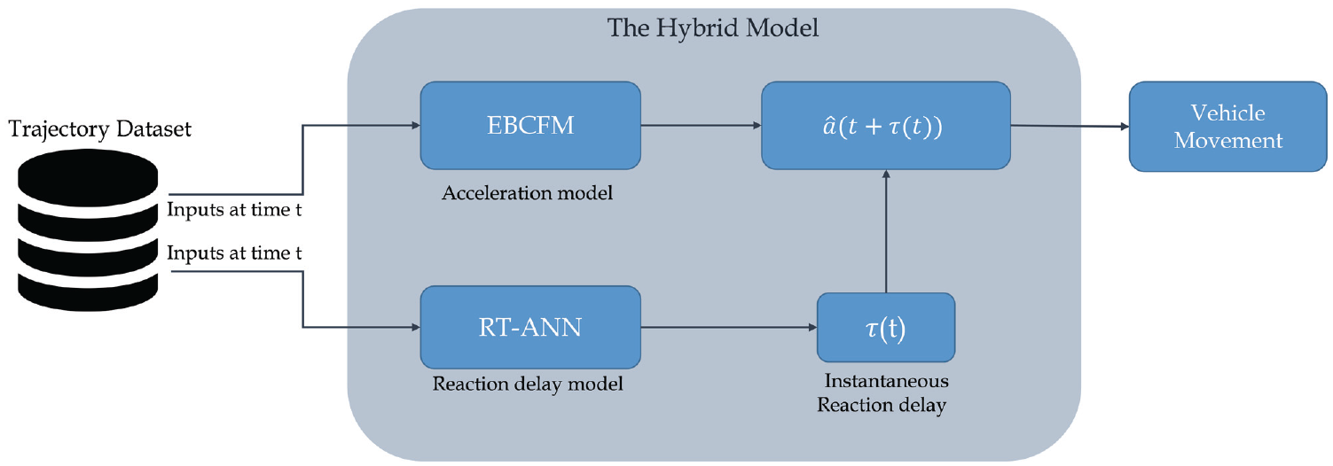
The general overview of the proposed hybrid framework.
It is worth noting that the expected acceleration can only be reached at
Figure 3 shows how to calculate the acceleration (and subsequently the speed) of the follower in four successive time steps. As can be seen, at time
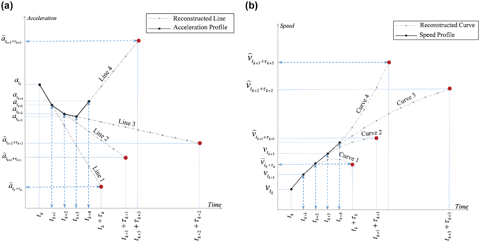
Calculation of acceleration and speed of follower by using reconstructed lines in successive time steps: (a) acceleration and (b) speed.
In the following sub-sections, the major components of the hybrid model (including EBCFM and RT-ANN), as well as the calibration configuration for the estimation of the model parameters, are briefly introduced.
The Acceleration Model (EBCFM)
Because of the generality of the proposed framework, almost any EBCFM can be integrated into it. However, for the sake of simplicity, the General Motors (GM) car-following model, as a popular member of the stimuli–response family of car-following models, is used in this study. Stimuli–response car-following models, which were first developed by researchers at GM, are one of the well-known models and have been studied more than any other car-following model. The basic equations of these models have been formulated based on the idea that a driver’s response to its leader’s behavior is proportional to the perceived stimulus with a proportionality constant called sensitivity. Therefore, the general form of these models can be written as Equation 1 ( 19 ):

By considering the relative speed and acceleration of the leader as, respectively, the stimulus and response, and a fixed value for the sensitivity factor, the simplest type of stimuli–response models (a linear car-following model) is achieved ( 20 ). Over the years, various forms of the sensitivity factor have been recommended. In this study, a specific form of the GM car-following model is used, which is formulated as in Equation 2:

where
RT-ANN
Artificial neural networks are parallel and interconnected networks of simple elements (usually adaptive) in which the hierarchical structure is intended to interact with the objects of the real world in the same way as biological nervous systems do (
21
). Neurons are the smallest units of information processing in neural networks. Figure 4a shows a typical neuron with n inputs. Elements of a neuron consist of weighted communication links, a summation function, a bias, and a transfer function (activation function). In an artificial neuron, each input x
i
is assigned a weight

where xi is the ith input, wi denotes the weight of the input xi, b is the bias, f is the activation function, and n is the number of inputs.
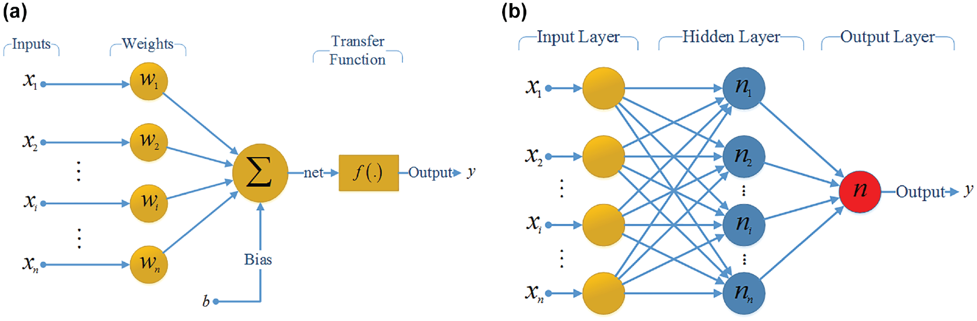
Artificial neural networks: (a) artificial neuron and (b) multilayer neural network.
Various types of neural networks can be utilized in the proposed structure. However, again for straightforward illustration, a multilayer perceptron (MLP) neural network, as one of the most popular families of neural networks, has been employed in this study. In MLPs, all neurons of a layer are connected to all neurons of the next layer. This arrangement forms a so-called full-connected network. Figure 4b shows a three-layer perceptron neural network (an input layer, a hidden layer, and an output layer). As can be seen, in this structure, each neuron in a layer is connected by weighted links to the neurons of the next layer, and the outputs of each layer are considered as the inputs for the next layer. The mathematical form of this neural network is as Equation 4:
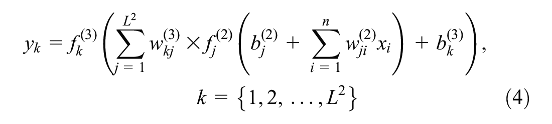
where
The three-layer neural network constructed in this study takes four variables as inputs at time t, including the speed of the subject vehicle (the follower), the relative speed between the follower and the leader, the space gap between the two vehicles, and the acceleration of the leader. The hidden layer consists of five neurons with a hyperbolic tangent sigmoid activation function, and the output layer contains one neuron with a logarithmic activation function. Figure 5 shows the mentioned activation functions. Based on the asymptote of the activation function in the output layer (Figure 5b), the estimated reaction time by the RT-ANN varies in the range of 0 to 2 s.
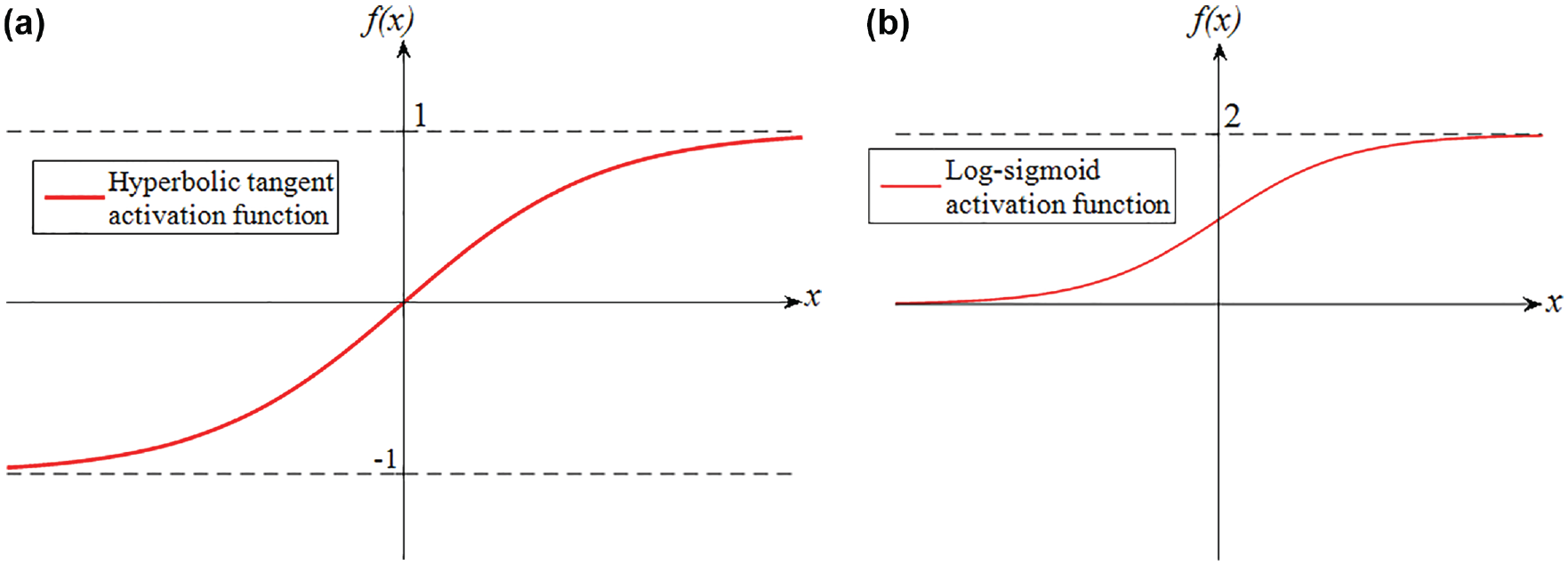
The activation function: (a) hyperbolic tangent and (b) logarithmic.
The Calibration Configuration
The adjustment of model parameters is a crucial step in developing any car-following model. For the proposed hybrid model, these parameters include the parameters of the EBCFM and the weights and biases of the artificial neural network (RT-ANN). In this study, it is assumed that reaction time has a hidden nature, and therefore no definition for calculation of the reaction time by using field observations has been carried out. In other words, reaction time observations (the training data) are not available, and adjustment of the RT-ANN model parameters by using traditional methods (such as minimum gradient and backpropagation) is not feasible because of the impossibility of direct comparison between the actual values of reaction time and the results of the RT-ANN model. Accordingly, an indirect method is applied for estimating the model parameters. In this method, which is referred to as joint estimation, all parameters of the model, including the parameters of EBCFM and RT-ANN, are calibrated simultaneously in a simulation-based optimization process. The whole calibration process is defined as a multivariate non-linear optimization problem in the form of Equation 5:

where

where
Figure 6 shows the general process of model calibration. As can be seen, the parameters of EBCFM and RT-ANN are considered as a vector to be adjusted using the EDA in a simulation-based optimization process. Accordingly, the initial population of solutions, by assuming that each parameter has a uniform distribution, is generated, and each solution is evaluated by its corresponding objective function value. Then, a certain number of individuals (promising solutions) are selected by using a selection method. These promising solutions will be used to construct the probabilistic model. In the next step, induction of the n-dimensional probabilistic model among the individuals of the previous step that best reflects the interdependencies between decision variables (model parameters) is carried out. This step is known as the learning step. After constructing the probabilistic model, new individuals are generated by sampling from the probabilistic model, and then the new population is generated by using a replacement method. The mentioned process is repeated until a certain stopping criterion is satisfied. More details in relation to the applied EDA can be found elsewhere ( 22 , 24 ).
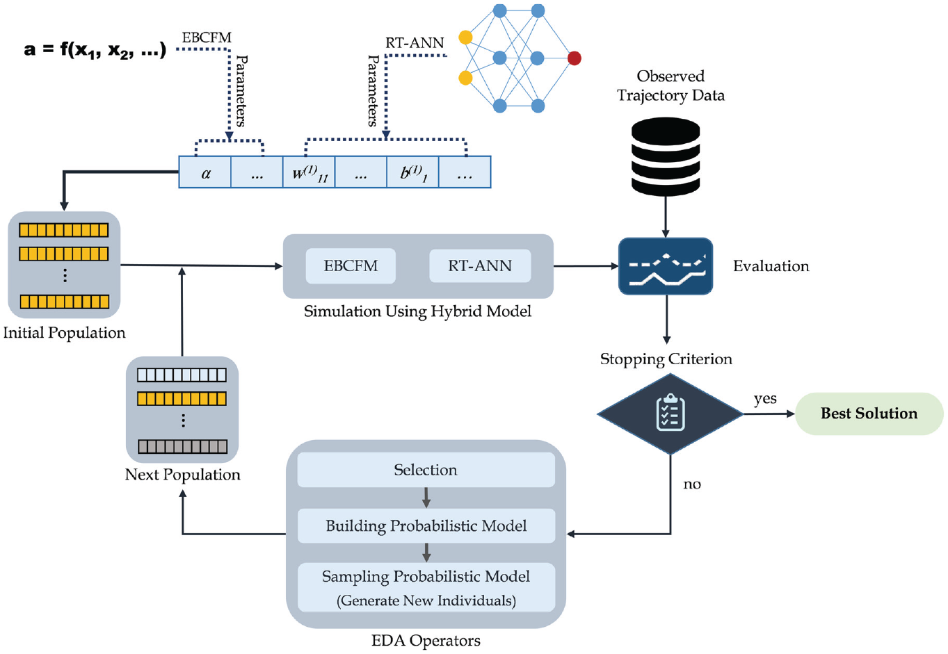
The general process of model calibration.
It is worthy to note that in this process, a complete observed trajectory is compared with a simulated trajectory in relation to the objective function. This method, which is also referred to as global optimization, is more reliable and robust than local approaches as a result of the propagation of errors between the observed and simulated data (as shown by Treiber and Kesting [ 25 ]). This leads to a lower risk of overfitting and thus, further generalizability of the model.
Furthermore, it should be noted that some solutions in the calibration process could lead to unusual driving behaviors such as high deceleration/acceleration or negative gaps (crash occurrence). Therefore, to reduce the attraction of such solutions in the applied optimization algorithm, a penalty term is added to the objective function value depending on the amount of violation.
Measure of Performance (Evaluation Criteria)
If a model can accurately reproduce the real system, or in other words, if there is no difference between the outputs of the model and the observations, the type of effectiveness criteria and the selected objective function have no impact on the estimated values of parameters. However, as models are tabloids of real systems, they are more or less accompanied by errors. Therefore, selecting different effectiveness criteria with the same objective function and even with the same optimal values of the objective function may lead to different estimations of the model parameters ( 22 , 26 ). In general, any time-varying quantity, such as the gap, speed, and acceleration, can be used as a measure of performance. In this study, gap is used as an appropriate quantity in the calibration process because any reduction in errors associated with the gap automatically leads to a reduction in the differences between observed and simulated values of speed ( 27 ).
Results
Performance of the Model
To compare the performance of the constructed hybrid model with its base model (the GM model), 84 pairs of vehicles were randomly selected from the US101 dataset, ensuring that they are affected by at least one shockwave and their travel times are longer than 60 s. For each pair of vehicles, both the hybrid model and the GM model have been calibrated, and the overall performance of them has been evaluated based on the average value of errors in relation to gap, speed, and acceleration. Table 1 shows the corresponding mean values of RMSE; α, β, and γ (the parameters of EBCFM); and estimated reaction delay. As can be seen, the average values of RMSE for the gap, speed, and acceleration for the hybrid model are, respectively, 23, 22, and 35 percent less than those for the GM model.
Calibration Results for the Hybrid and GM Models
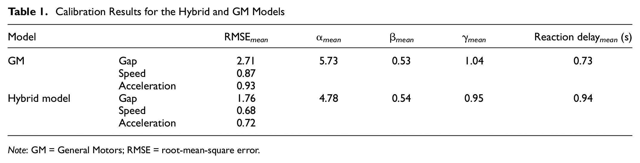
Note: GM = General Motors; RMSE = root-mean-square error.
For a more visible comparison, the cumulative distributions of RMSE values for the two models have been depicted in Figure 7. It can be seen that the RMSE values for the hybrid model are lower throughout the distribution. For 95% of the calibrated hybrid models, the error values are less than 0.9, 0.9, and 2.5, respectively, for the acceleration, speed, and gap, while the corresponding values for the GM models are 1.4, 1.3, and 4.6. The results of the two-sample Kolmogorov–Smirnov test and the corresponding p-values are also presented at the top of each plot. As can be seen, the null hypothesis, H0 (RMSE values for the hybrid and GM models have been taken from the same distribution), is rejected with a p-value = 0.00 for all evaluation criteria, indicating a better performance of the proposed model. Previous studies have shown significant variations in the performance of car-following models dealing with different drivers and even with one driver in different conditions ( 26 , 28 ). These variations are linked to the inability of traditional models in depicting some aspects of driving behavior. Variability of drivers’ reaction delay during the driving task is one of the most important of such aspects. The ability of the hybrid model to account for these variations decreases the range of RMSE values for different drivers compared to the GM model (as illustrated in Figure 7).
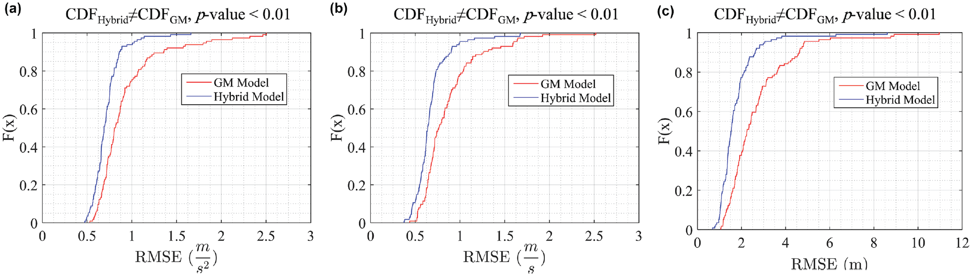
Cumulative distribution of RMSE values for (a) acceleration, (b) speed, and (c) gap.
Figure 8 illustrates the box plots of the estimated reaction delays resulting from the calibration of the hybrid and GM models, as well as those resulting from the model of Ozaki ( 15 ) and the neural network model provided by Zheng et al. ( 4 ). The differences in variation ranges of reaction time among the four mentioned models are apparent. The interquartile range for the hybrid model is approximately 1.24 s, and the corresponding values for the GM, Ozaki’s, and Zheng’s models are 1.0, 0.15, and 0.11 s, respectively. Lower amplitudes of the reaction delay resulted from the models of Ozaki ( 15 ) and Zheng et al. ( 4 ) could be because of their applied methodologies for calculating the driver’s reaction delay. In their approaches, it is impossible to extract sufficient data from the trajectory of an individual driver and his/her leader to construct a disaggregated model. Therefore, these models are developed at an aggregate level by using trajectories from different pairs of vehicles. In fact, for each specific traffic condition, they are predicting an average driving behavior and reaction delay. Contrarily, in the proposed hybrid model, the consideration of reaction delay as a hidden variable and the joint estimation of all model parameters provide the feasibility of building a model at the individual scale (disaggregate level), thus allow taking the heterogeneity among drivers more appropriately into account.
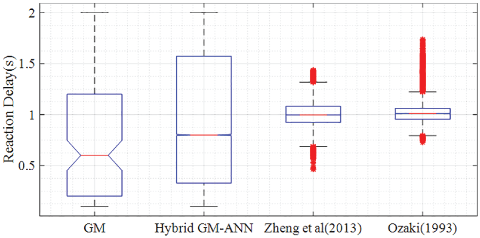
Comparison of simulated reaction delay resulted from Hybrid GM-ANN, GM, Ozaki’s, and Zhang’s models.
To investigate the variations of the models’ parameters, the boxplots of the corresponding values for the hybrid and GM models are presented in Figure 9. In general, this variation results from differences in driving behavior among drivers ( 29 ). However, as can be seen, the variability of α in both models is higher compared with β and γ, which is in agreement with previous studies ( 26 ). The variation range of α in the calibrated GM models is distinctly different from that in the hybrid models. 50% of α values in the GM models vary from 5.1 to 7.0, whereas the corresponding values are in the range of 3.7 to 6.0 for the hybrid models. This is because the parameter α in the GM model represents different aspects of the driving task that are not considered by the model (including the variability of reaction time) and are primarily reflected in the constant coefficient. Therefore, considering the instantaneous reaction time in the hybrid model affects the magnitude of α more than other parameters. Variation ranges of β and γ for both models are almost similar; however, the outliers are less frequent in the hybrid models.
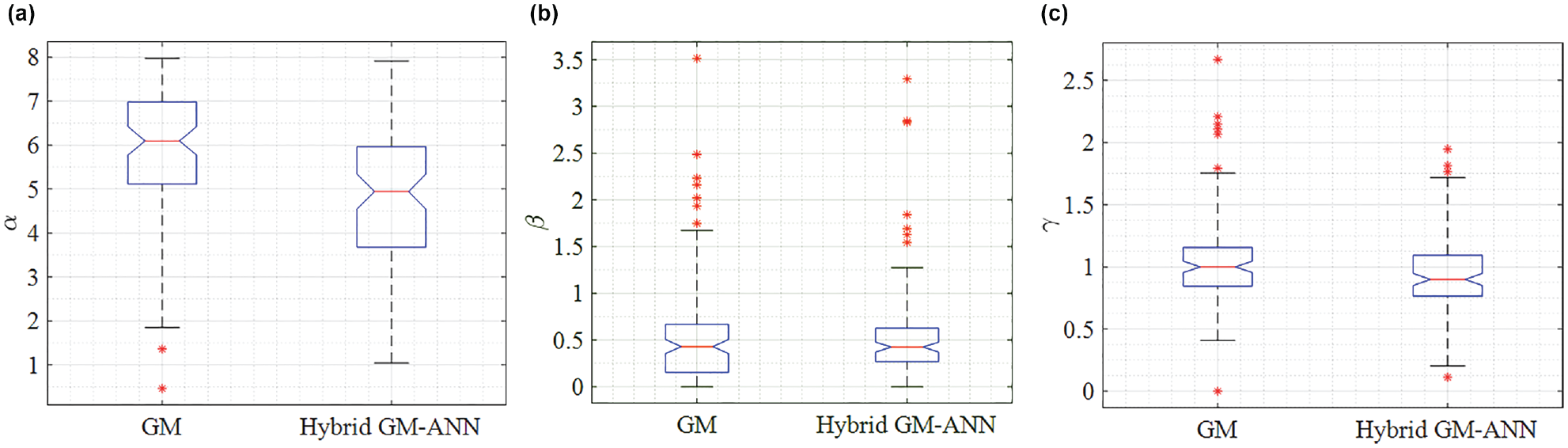
Boxplots of estimated parameters for the Hybrid GM-ANN and GM: (a) α, (b) β, and (c) γ.
It should be noted that the upper extreme value in the α-diagram and the lower one in the β-diagram respectively correspond to the maximum and minimum allowable values for these parameters in the calibration process. Therefore, it is possible that better results are achieved by changing these thresholds. However, the number of cases that hit the specified boundaries is limited because of the wide range of parameters in the calibration process.
Rationality of the Model
Figure 10 illustrates the acceleration, speed, and gap profiles extracted from field observations as well as those estimated by the hybrid and GM models calibrated for a specific vehicle (vehicle ID: 661). It can be seen that the trajectory data simulated by the hybrid model are more consistent with the observed data. The calculated errors, based on Equation 6, for the acceleration, speed, and gap are 0.59, 0.5, and 2.4 for the GM model; and 0.47, 0.37, and 1.0 for the hybrid model, respectively.
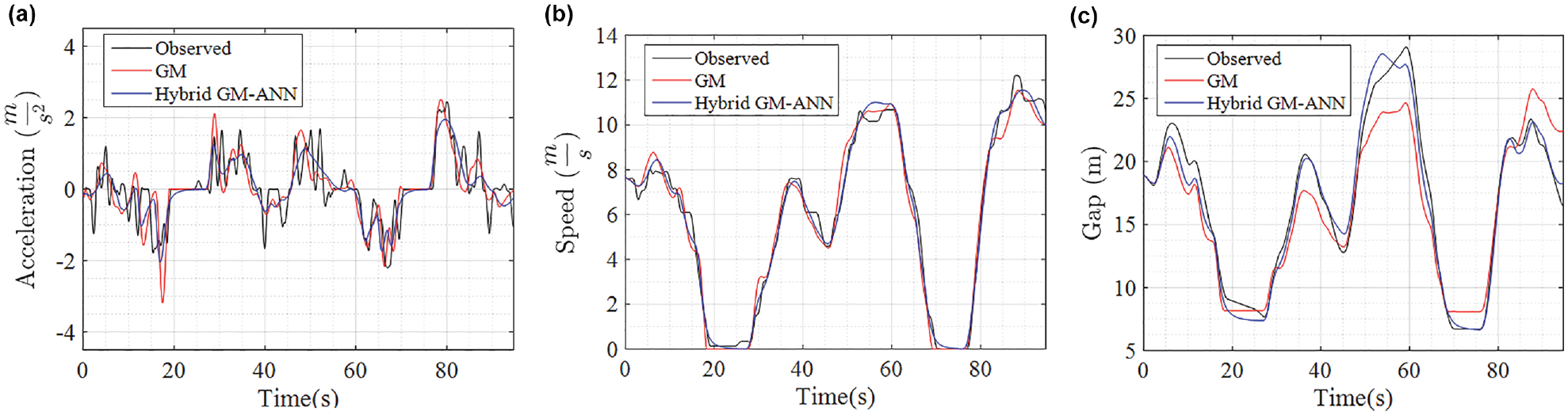
Comparison between the (a) acceleration, (b) speed, and (c) gap resulting from the calibration of GM and Hybrid GM-ANN models with the actual trajectory.
To scrutinize RT-ANN (the reaction time estimation part of the model), the time series of reaction delay estimated by the hybrid model and the one estimated by the model of Ozaki ( 15 ) (calibrated for US101 by Zheng et al. [ 4 ]) have been illustrated in Figure 11. The general trends of the driver’s time delay are similar in both models. However, the variation range of reaction time resulting from the model of Ozaki ( 15 ) is smaller and is confined to [0.85–1.15], while for the hybrid model, it is limited to [0.3–2.0]. It should be noted that the reaction time that is calibrated by the GM model is a constant value and equals 0.6 s.
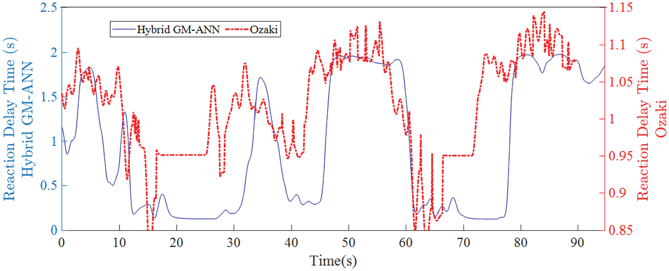
The time delay calculated by the Hybrid GM-ANN and Ozaki models (vehicle ID = 661).
It can be seen that the reductions in the gap magnitude (Figure 10c) are accompanied by the decreases in the driver’s reaction delay (Figure 11), and vice versa. This is almost consistent with what is perceived through driving experience. Small headways usually occur in congestion situations. Under such circumstances, drivers are usually more cautious and carefully follow the changes in their surroundings and can even predict these changes. In addition, based on their experiences in different traffic conditions, they are aware of possible, sudden changes of speed resulting from shock waves or behaviors of some aggressive drivers, and consequently focus more on driving. This predictive behavior and the greater attention to the driving task lead to a reduction in the driver’s reaction delay in response to the surrounding stimuli. Conversely, when the gap is relatively large, the driver might not show urgency to react to the surrounding traffic. Furthermore, considering the fluctuations of reaction time, the time series derived from the model of Ozaki has irregular fluctuations that seem to be far from reality.
Figure 12 presents the scatter plots of relative speed (speed of the leader minus the follower’s) versus acceleration/deceleration for both real observations and the simulation results of the hybrid and GM models. As can be seen in Figure 12a, although most of the observed accelerations are located in the range of positive relative speeds, a significant portion lies in the range of negative relative speeds, where the speed of the follower is higher than the speed of the leader (quadrant II). Similarly, a good portion of deceleration observations is located in the range of positive relative speeds (quadrant IV). Moreover, a significant amount of data are located along the horizontal axis, where the acceleration of the follower equals zero, but the relative speed does not. These observations are consistent with the findings of Koutsopoulos and Farah ( 30 ) and are in contrast with previous modeling approaches, which assume that a driver decelerates when the relative speed is negative, and vice versa. This could be related to the limitations of drivers’ perception, that is, when there are small speed differences between the two vehicles, the following driver is not able to detect the differences correctly; consequently, the application of acceleration/deceleration is to a large extent random in such situations. Therefore, at low relative speeds, these points are usually randomly scattered around the origin of the coordinate system. Another justification could be related to the drivers’ temporal and spatial prediction ability and, subsequently, their variable reaction delay in response to stimuli. For example, it is possible that the gap between the two vehicles is about to decline, but according to the surrounding traffic conditions, the driver predicts an increase in the gap in the near future, and based on this prediction, may postpone the deceleration (which leads to larger reaction delay), extend its duration, or reduce its intensity. Postponing the acceleration/deceleration, as it is clear in real data, has led to the placement of some points in parallel and close to the horizontal axis. The mentioned phenomena are partly considered by the hybrid model as a result of applying the RT-ANN model, which leads the simulation results of the proposed model (Figure 12b) to be more consistent with the field observations (Figure 12a) in comparison to the outputs of the GM model.
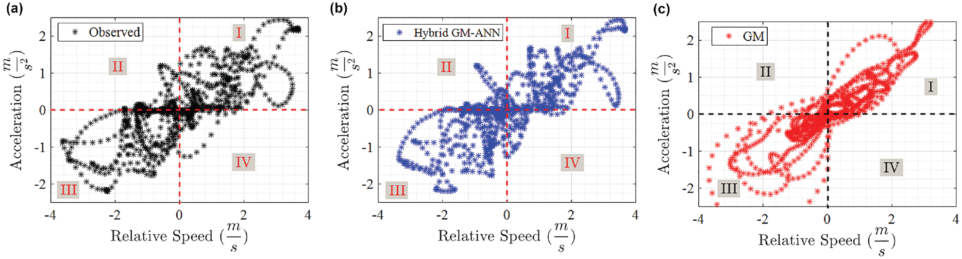
Scatter plots of relative speed versus acceleration for the vehicle with ID = 661: (a) observed, (b) hybrid GM-ANN, and (c) GM.
Generalizability of the Model
In practice, car-following models are used to predict the following behavior of a driver beyond the traffic conditions under which they have been calibrated. Therefore, assessment of the accuracy, transferability, and generalizability of such models is crucially important. A simple method for such evaluation is cross-validation ( 31 ). The idea is to validate the model calibrated for each vehicle by simulating the driving behavior of other vehicles that did not exist in the calibration process. In this regard, first, a hybrid model is calibrated based on the trajectories of a specific pair of vehicles; then, the constructed model is validated by the trajectories of the other 83 pairs of vehicles. Similarly, we calibrate a new model based on the trajectories of the second pair of vehicles and validate this model by using the trajectories of the other 83 pairs. We repeat this process for all pairs of vehicles, which means at the end, we have 84 models, each of which has been validated against 83 trajectories that were not used in the calibration process. For each calibrated model, the RMSE values for the speed, acceleration, and gap are calculated for each pair of vehicles in the validation set based on the differences between the real and simulated trajectories. Finally, the cumulative distributions of these RMSE values are used to evaluate the model performance. Investigating the cumulative RMSE distributions for some vehicles indicates that the hybrid model outperforms the GM ones in the cross-validation process. Figure 13 shows the cross-validation results for one vehicle (vehicle ID: 1729) as an instance of these cases. However, for a limited number of vehicles, the GM model’s performance in reproducing the gap profile is more appropriate in the cross-validation process (Figure 14, vehicle ID: 1584).
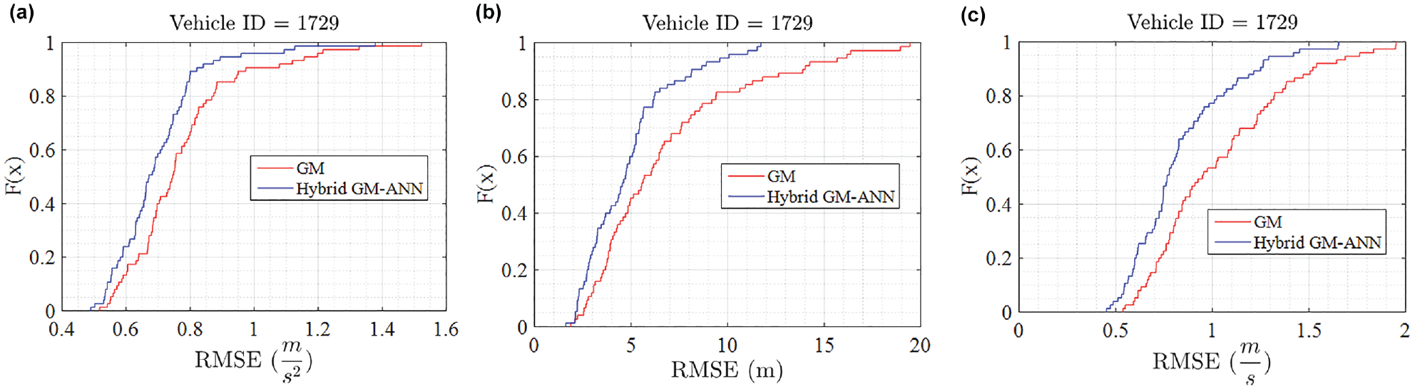
Cumulative distribution of errors in cross-validation based on the calibrated parameters for the vehicle with ID = 1729: (a) acceleration, (b) speed, and (c) gap.
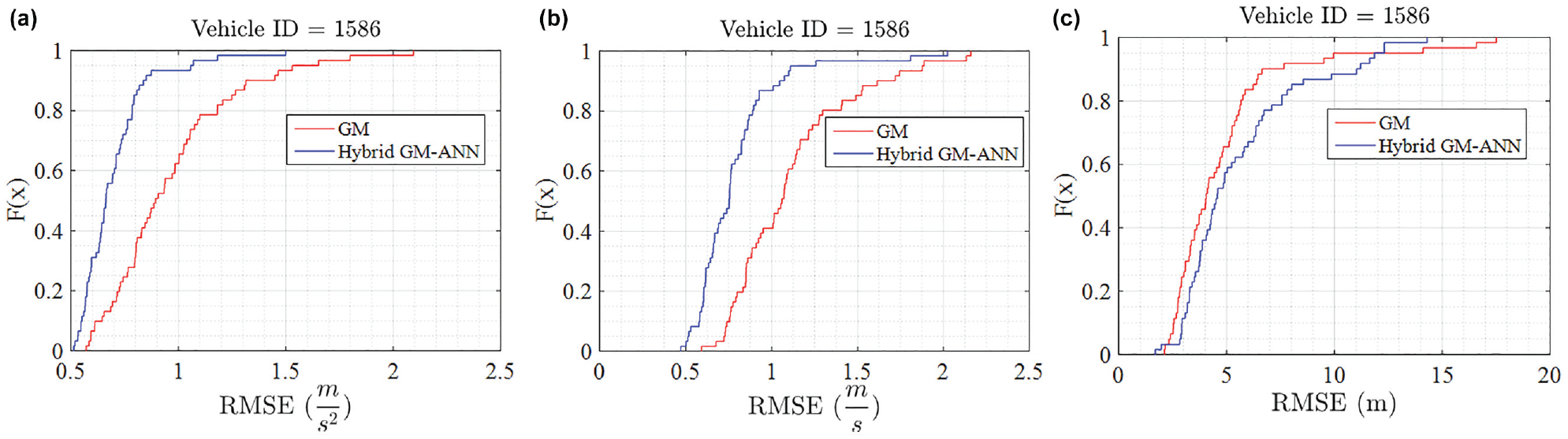
Cumulative distribution of errors in cross-validation based on the calibrated parameters for the vehicle with ID = 1586: (a) acceleration, (b) speed, and (c) gap.
To evaluate the overall performance of the two models, the average of RMSE values resulted from each cross-validation is calculated, and the cumulative distribution of these average values has been depicted in Figure 15. Using the nonparametric Kolmogorov–Smirnov test, the null hypothesis, H0, is rejected for the distribution of mean RMSE values for the acceleration and speed (p-value = 0.00). However, for the mean RMSE distribution of the gap, the null hypothesis is not rejected at 95% confidence level (p-value = 0.067). Accordingly, the cumulative distribution of RMSE resulted from the cross-validation, as a statistical representation of accuracy and generalizability, indicates that the hybrid model has been more successful in reproducing the speed and acceleration profiles of vehicles that were not included in the calibration process. However, both models have shown relatively similar performance in reproducing the gap profile. It is worth mentioning that using the calibrated parameters of one vehicle for simulating the other vehicles’ car-following behavior led to accidents in both models in some limited cases. These cases were removed from the validation process.
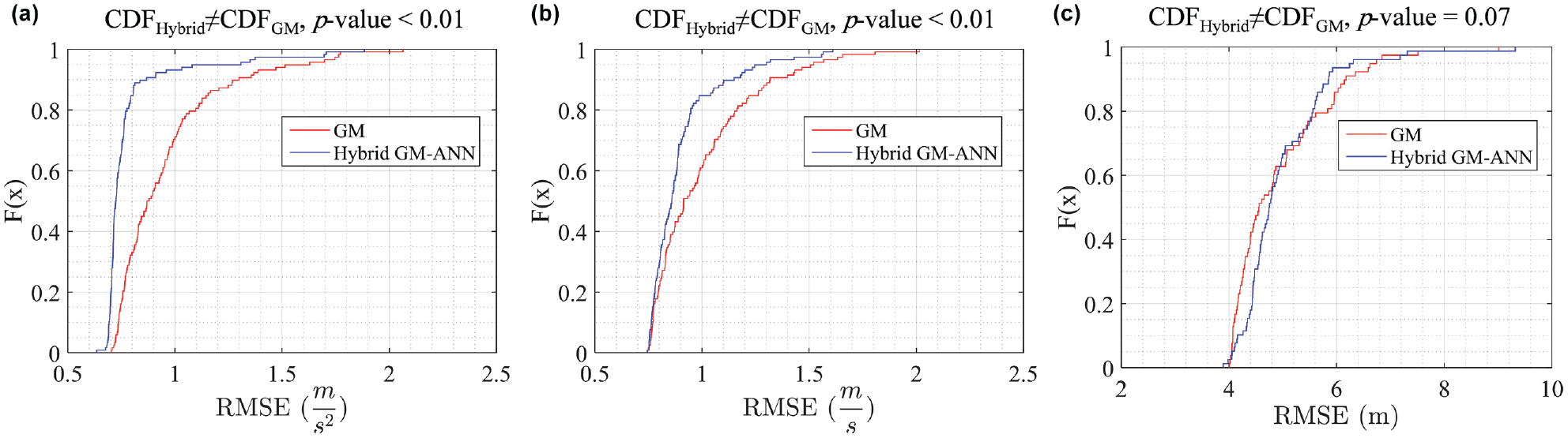
Cumulative distribution of errors based on the average value of RMSE for cross-validations: (a) acceleration, (b) speed, and (c) gap.
Conclusion and Future Study
Car-following is one of the main driving behaviors and has considerable impacts on the performance of traffic flow, road safety, and pollution emission. Models describing such behavior are crucial components of traffic microsimulation tools. The accuracy of these tools, to a large extent, depends on the performance of their car-following models. Several factors affect car-following behavior, and drivers’ reaction delay in response to the surrounding traffic conditions is one of the most important of such factors. Because of its hidden nature, reaction delay is considered constant in traditional car-following models, whereas it is a complex phenomenon, influenced by many parameters, and varies during the driving process. Therefore, assuming a fixed value in the whole process of driving does not seem to be appropriate.
In this paper, a hybrid approach is proposed that enables the integration of instantaneous reaction delay into traditional, EBCFMs. In this framework, first, the desired acceleration of the driver is estimated using an EBCFM. Then, the driver’s delay in applying the estimated acceleration is calculated by employing an artificial neural network (RT-ANN). Parameters of the EBCFM, as well as the weights and biases of the RT-ANN model, are jointly estimated in a simulation-based optimization process by using an EDA as the solution algorithm. The comparison between the proposed hybrid model and its traditional competitor indicates the better performance of the proposed model in describing the car-following behavior. The conducted cross-validation to assess the generalizability and transferability of the hybrid model also indicates its satisfactory performance. It is worth noting that the proposed framework is relatively general, and a wide range of traditional car-following models could be integrated into that.
Despite the promising results of the developed hybrid model, there are some improvements that could be considered in future studies; for instance, adopting advanced machine learning techniques, such as convolutional neural networks, for taking into account the effects of peripheral conditions and drivers’ spatial and temporal predictions, and employing more efficient calibration configurations, considering the high complexity of joint estimation of model parameters. Also, incorporating more recent car-following models into the proposed hybrid structure and testing the hybrid model in different car-following scenarios could be of interest.
Footnotes
Acknowledgements
The authors would like to thank Traffic Research Laboratory of Iran University of Science and Technology (IUST-TRL) for hardware and software support and NGSIM for providing trajectory datasets.
Author Contributions
The authors confirm contribution to the paper as follows: study conception and design: M. Rafati Fard, S. Rahmani, A. Shariat-Mohaymany; data collection: M. Rafati Fard; analysis and interpretation of results: M. Rafati Fard, S. Rahmani, A. Shariat-Mohaymany; draft manuscript preparation: M. Rafati Fard, S. Rahmani, A. Shariat-Mohaymany. All authors reviewed the results and approved the final version of the manuscript.
Declaration of Conflicting Interests
The author(s) declared no potential conflicts of interest with respect to the research, authorship, and/or publication of this article.
Funding
The author(s) received no financial support for the research, authorship, and/or publication of this article.