Exploring Taxi Demand Distribution of Comprehensive Land-Use Patterns Using Online Car-Hailing Data and Points of Interest in Chengdu,China

Abstract

With the rapid advance of urbanization, land-use intensity is increasing, and various land-use forms gather to form comprehensive land-use patterns. Traffic demand shows variability and complexity under comprehensive land-use patterns. Accurate analysis of traffic demand in urban transportation is the key to active traffic control and road guidance. Researchers have widely studied the relationship between traffic demand and land-use patterns, while land-use intensity is ignored when classifying land-use patterns, and the traffic demand distribution in each land-use pattern is not studied specifically. Taxi is a flexible public mode in urban areas, and taxi demand is an important component in analyzing traffic demand and identifying traffic hotspots in cities. This paper explores taxi demand distribution of comprehensive land-use patterns using online car-hailing data and points of interest (POI) in Chengdu, China. The demand-driven traffic analysis zones are developed by clustering origin–destination points of online car-hailing services. Using POI data, comprehensive land-use patterns are classified with land-use forms and land-use intensity. The K-shape algorithm is adopted to extract the typical taxi demand distribution in each comprehensive land-use pattern. Finally, two indicators, total taxi demand (TTD) and taxi demand difference (TDD), are computed and further analyzed. Results show that taxi demand distribution is still differential even under the same land-use pattern. Three land-use patterns whose average hourly taxi demand reaches about 300 vehicles per square kilometer have the largest TTD and most uneven TDD. The findings can support traffic management, land-use combination, and land-use adjustment to avoid concentrated taxi demand and mismatched TDD.

Accompanied by the rapid advance of urbanization in the past decades, land-use intensity has increased significantly. Various land-use forms gather to form comprehensive land-use patterns, providing greater convenience for people’s lives. However, early urbanization is mostly spontaneous and unplanned, leading to irrational urban structures and further causing cities to suffer from serious problems such as traffic congestion and residential inconvenience ( 1 , 2 ). Urban land-use patterns are key to determining the traffic demand distribution ( 3 , 4 ). Understanding the relationship between land-use patterns and traffic demand is considered an effective way to solve the existing urban problems ( 5 – 7 ).

To clarify the influence of land-use patterns on traffic demand, numerous scholars have studied the interaction between land-use patterns and travel behavior based on the traditional travel survey. Gao et al. ( 8 ) made a detailed analysis of travel distance and travel time under various travel purposes through a household travel survey in Qingdao, China. Similarly, Currans and Clifton ( 9 ) estimated traffic generation based on the household travel surveys in Oregon, Washington, and Maryland, and found that comprehensive land-use patterns enhance residents’ travel demand and induce higher traffic generation. Conclusions from the existing research ( 10 – 12 ) also show a strong correlation between the land-use forms of origin–destination and travel purposes.

Nevertheless, traditional travel surveys are costly and time consuming, with low response efficiency and accuracy, meaning that they can only be conducted in a short period or a limited area. Accordingly, the findings based on travel surveys cannot fully reveal long-term travel patterns or provide sufficient information for traffic planning ( 13 , 14 ). At present, various methods for recording the travel information of vehicles have been developed with communications technology, such as GPS ( 15 , 16 ). Compared with the traditional travel surveys, these novel datasets have outstanding advantages in high volume, high accuracy, detailed information, and long-term detection ( 17 ). Electronic map systems have also become prevalent with the booming use of mobile electronics. Points of interest (POIs) on the electronic map can provide land-use information for individuals to access expected services, which provides a novel approach to distinguishing and classifying land-use forms ( 18 , 19 ).

The use of POIs reveals that current land-use forms are developing toward diversification and mixing. Thus, considerable efforts have been devoted to investigating the influence of different land-use forms on daily traffic demand. Lin and Yang ( 20 ) indicate that land-use intensity is positively related to trip generation and negatively associated with mode split. Wang et al. ( 21 ) found that locations with the best accessibility for driving, cycling, and walking tend to have residential and commercial uses. Industrial use prefers locations with high driving accessibility. Furthermore, various land-use forms tend to gather and form comprehensive land-use patterns; that is, various land-use forms, rather than only a single land-use form, are located in the same area. Taking the residential area as an example, land-use forms, including shopping, leisure, schools, hospital, station, and so forth, are often located around it. Classifying land-use patterns has become an important part of studying problems related to land use, especially when it comes to comprehensive land use. Bao et al. ( 13 ) divided the land-use forms in New York into five patterns with K-means clustering algorithm according to the proportions of six POI categories. Similarly, seven land-use patterns were classified by using the Delphi method to calculate the functional attributes of each community in Chengdu ( 22 ).

Using the recorded travel information, traffic demand is usually extracted and analyzed based on traffic analysis zones (TAZs). During this process, the modifiable areal unit problems (MAUP) have been widely studied, which are directly or indirectly related to traffic demand analysis through the design of TAZs ( 23 – 27 ). The current TAZs mainly arise from regular grids ( 26 ) or some existing geographic schema designed for postal service or administration ( 27 ), which have limitations in considering the spatial distribution of origin–destination points ( 28 ). For TAZs arising from a regular grid, it is difficult to determine the division parameters because of the complexity, which also restricts its application ( 29 ). To avoid these issues, traffic demand distribution is recognized as an important factor relevant to the design of TAZs, including the shape and area of the TAZs ( 30 ). The use of demand-driven TAZs can be understood as an effort to solve the MAUP and improve the accuracy of traffic demand distribution analysis.

Although the relevant works of traffic demand distribution have been well studied, there are also some limitations: (i) TAZs mainly arise from regular grids or some existing geographic schema designed for postal service or administration, which are limited in considering the spatial distribution characteristics of origin–destination points; (ii) comprehensive land-use patterns are determined only with the proportions of various land-use types, ignoring the effect of land-use intensity and lacking the alternative index of land-use intensity; (iii) traffic demand under the same land-use pattern is analyzed aggregately in the previous research. Nevertheless, traffic demand distribution is affected by multiple factors. Even under the same comprehensive land-use pattern, traffic demand distribution will also be differential, which is neglected in the existing research.

The urban transportation system is composed of various traffic modes, such as private cars, taxis, buses, subways, and non-motorized modes. It is difficult to obtain the travel records of all traffic modes and extract an overall traffic demand accurately. As a flexible public mode without fixed routes in the city, use of taxis is not restricted by ownership of vehicle or driver’s license, climate/weather, fixed operating time or routes compared with private cars, non-motorized modes, buses, and subways. Besides, traveling by taxi has almost no access distance, which is appropriate to extract taxi demand accurately. Taxi demand cannot be a proxy of overall urban traffic demand, specifically, taxi demand is much higher at higher-value locations such as transportation hubs and downtown areas compared with the lower-value locations such as residential areas. Nevertheless, taxi demand is still an important component of overall traffic demand and is helpful to identify traffic hotspots in the city. As a novel dataset collected through positioning sensors, online car-hailing data which records accurate travel time and position has been widely used to extract travel patterns ( 15 , 31 ), identify traffic congestion ( 32 , 33 ), evaluate network reliability ( 34 ), and analyze traffic demand ( 35 , 36 ).

This paper aims to explore the taxi demand distribution of comprehensive land-use patterns using online car-hailing data and POI data. Based on the limitations identified in the literature review above, this paper makes the corresponding efforts. (i) Demand-driven TAZs are developed by clustering the positions of origin–destination points. Specifically, each TAZ corresponds to one cluster of taxi demand, avoiding the limit that different clusters of taxi demand are included in the same TAZ, or one cluster of taxi demand is divided into different TAZs. (ii) Land-use intensity and the proportion of various land-use categories are used together to classify the comprehensive land-use patterns. (iii) The time-series clustering method is developed to further extract the typical taxi demand distributions in each comprehensive land-use pattern, and spatiotemporal characteristics of typical taxi demand distributions are discussed in detail. The findings are prospective to provide suggestions for traffic management, land-use combination, and land-use adjustment to avoid the concentrated taxi demand and mismatched taxi generation/attraction.

This paper is organized as follows. The next section exhibits the data sources. The third section introduces the methodology of this paper. The data analysis and results are presented in the fourth section. The final section develops a conclusion of the finished work and points out the direction for future research.

Data Sources

The research area of this paper is located in Chengdu, China. Data sources, including online car-hailing data and POI data, are introduced, and the data preprocessing is explained in this section, providing support for the following data analysis.

Study Area

Chengdu, the capital of Sichuan Province, is located in the southwest of China. Its geographical coordinates are $102^{°} 54' ~ 104^{°} 53'$ longitude and $30^{°} 05' ~ 31^{°} 26'$ latitude. Considering that the area of Chengdu is so vast and the intensity of land-use in different districts is diverse, an area with the Third Ring Road as the boundary (Figure 1a) is adopted as the study area, which is shown in Figure 1b, including the districts of Jinjiang, Jinniu, Qingyang, Wuhou, and Chenghua.

Figure 1.

(a) Administrative districts of Chengdu and location of the study area, and (b) network and boundary of the study area.

Data and Processing

Online Car-Hailing Data

The online car-hailing data used in this paper is provided by the Didi Company in China and was downloaded from the company’s website (https://gaia.didichuxing.com). In a departure from traditional car-hailing, the Didi Company has launched online car-hailing services. Passengers can actively issue travel orders by designating their origin and inputting the destination on the Didi online app. The control console will respond to each order and assign a nearby Didi taxi to pick up the passenger according to the real-time location of the Didi taxi collected by the vehicle’s GPS recorders. Passengers are able to access the travel service without walking to the roadside, they only have to wait for the Didi taxi at the designated origin, such as a residential building or community gate. In this way, the origin–destination information of all orders can be recorded and is more accurate compared with the traditional car-hailing data, avoiding the extra walking for taxi services, which provides a novel dataset for analyzing the taxi demand distribution.

Travel information on all orders of online car-hailing services whose origin and destination are located in the study area recorded from November 1, 2016, to November 30, 2016 was downloaded in this study. Unfortunately, the online car-hailing data for November 3 is missing on the website. Finally, a total of 29 days with 6,847,539 online car-hailing records were obtained. The dataset contains seven types of information: order ID, pick-up time, drop-off time, pick-up longitude, pick-up latitude, drop-off longitude, and drop-off latitude. The order ID is unique for each order and the latitude and longitude are under the WGS84 coordinate system.

There were no national holidays in November 2016, so the impact of holidays on taxi demand distribution is not included in this paper. To verify the difference between weekdays and weekends, the hourly taxi generation of weekdays and weekends is counted from the online car-hailing data according to the pick-up time, as shown in Figure 2, a and b , respectively. Some obvious differences in hourly taxi generation between weekdays and weekends can be seen. The taxi generation on weekdays has three peaks at 9:00 a.m., 1:00 p.m., and 5:00 p.m., respectively, while on weekends there is no peak of taxi generation at 9:00 a.m. The taxi generation in the morning on weekdays has a sharp increase at first, then goes down until midday. However, the taxi generation in the morning on weekends keeps increasing slowly. Considering the above difference, taxi demand distributions on weekdays and weekends are extracted separately in the following analysis.

Figure 2.

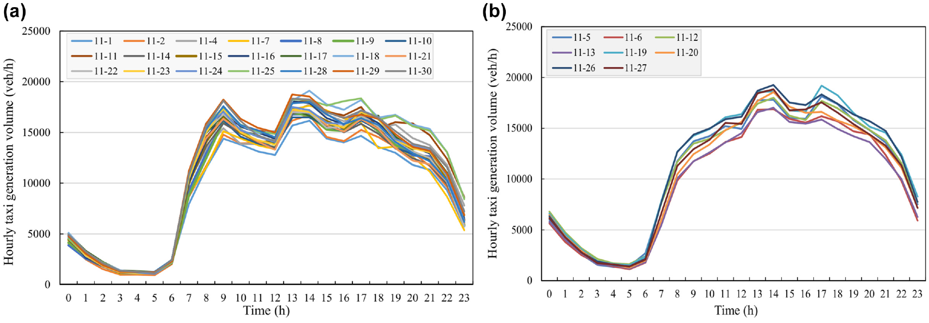
Hourly taxi generation (a) on weekdays and (b) on weekends. Each colored line is a day of the month of November 2016.

POI Data

This study downloaded all the POI data within the study area in Chengdu by the application programming interface (API) of Gaode Map (https://www.amap.com) to reflect the land-use characteristics. The data acquisition was conducted in November 2016, which is consistent with the travel date of the online car-hailing data. The POIs are divided into eight categories: Eating, Shopping, Life service, Health care, Residence, Education, Traffic, and Work. There are various types of POI in each category. The POI categories in Gaode Map and their proportions in the study area are shown in Table 1.

Table 1.

Points of Interest (POI) Category Classification and Downloaded Proportion

POI category	Proportion (%)	POI types
Eating (Ea)	19.41	Bar, café, food, meal delivery, meal takeaway, restaurant, canteen, milk-tea shop, etc.
Shopping (Sh)	25.68	Stores of shoes, clothes, books, electronics, furniture, supermarket, house goods, shopping mall, cinema, etc.
Life service (Ls)	22.75	Barbershop, laundry, beauty salon, internet bar, delivery, lottery, housekeeping, repair shop, etc.
Health care (Hc)	6.14	Hospital, clinic, pharmacy, sanatorium, acupuncture room, maternal and child health hospital, etc.
Residence (Re)	6.57	Commercial housing, affordable housing, villa, budget hotel, hotel, apartment, etc.
Education (Ed)	6.29	Primary school, middle school, university, college, coaching agency, children’s palace, etc.
Traffic (Tr)	2.14	Airport, bus station, subway station, taxi station, rail station, highway toll gate, park, etc.
Work (Wo)	11.02	Company, factory, office building, workshop, etc.

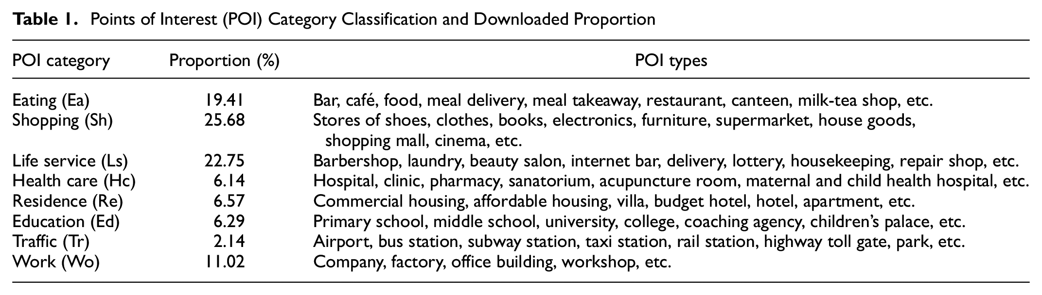
Finally, 462,946 POI data in the study area were downloaded, including the POI category, longitude, and latitude. From Table 1, the Shopping category accounts for the largest proportion, reaching 25.68%. However, the Traffic category only accounts for 2.14%. It is worth noting that the POIs of Residence are extracted with the location and name of unit buildings, such as a whole hotel and residential buildings, rather than unit apartment or house. Consequently, the proportion of Residence only accounts for 6.57%, which is a little more than 3.61% in the existing research ( 22 ) for classifying all kinds of hotels as Residence in this study. Besides, the latitude and longitude of POIs in the Gaode Map are under the GCJ-02 coordinate system. The authors transformed that coordinate system to the WGS84 system to remain consistent with the online car-hailing data.

Methodology

As discussed in the previous section, online car-hailing data and POI data were downloaded first. Then the origin–destination points of taxi orders were extracted, and clustering analysis applied to discover the clusters of taxi demand, denoted as TAZs in this study. Furthermore, POI data was matched with each TAZ to calculate the POI proportion and POI density. With POI proportion and POI density, clustering analysis was applied again to determine the typical comprehensive land-use patterns. After that, the hourly taxi demand for each comprehensive land-use pattern was extracted by recorded date and transformed into time-series. Finally, the K-shape algorithm was developed to explore these time-series characteristics and output the typical taxi demand distribution of each comprehensive land-use pattern. The flow diagram of the designed framework is shown in Figure 3. The clustering algorithm, K-shape algorithm, and clustering evaluation indexes used in this study are introduced as follows.

Figure 3.

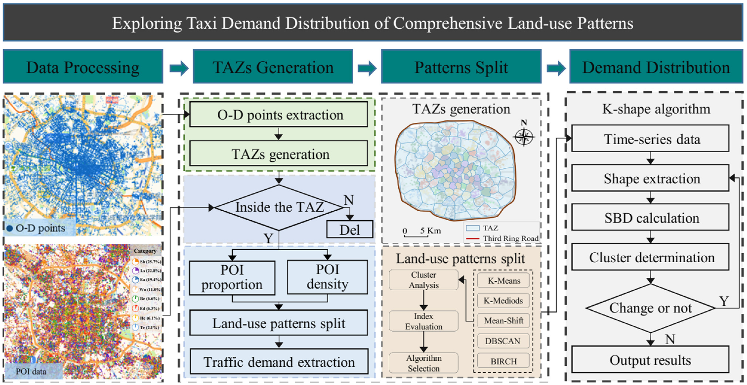
Flow diagram of strategy for exploring taxi demand distribution.

Clustering Algorithm

Clustering analysis divides the dataset into multiple clusters consisting of objects with the same characteristics. Generally, the traditional clustering algorithms can be divided into partitioning, hierarchical, and density-based methods ( 37 ). Among these, five typical clustering algorithms: K-means, K-mediods, BIRCH, DBSCAN and mean-shift, are chosen in this study, and a summary is presented in Table 2 ( 13 , 37 ).

Table 2.

Characteristics Comparison of Typical Clustering Algorithms

Clustering algorithm	Category	Time cost	Shape of dataset	Sensitive to noise	Parameter adjustment	Clustering interpretability
K-means	Partitioning	Low	Convex	Bad	Easy	Good
K-mediods	Partitioning	Middle	Convex	Moderate	Easy	Good
BIRCH	Hierarchical	Low	Convex	Moderate	Complex	Moderate
DBSCAN	Density-based	Middle	Arbitrary	Good	Complex	Bad
Mean-shift	Density-based	Middle	Arbitrary	Good	Complex	Moderate

K-Shape Algorithm

As mentioned above, time-series clustering is used to extract the typical taxi demand distribution of each comprehensive land-use pattern. In this study, the K-shape algorithm developed by Paparrizos and Gravano ( 38 ) is used, which proposes a normalized version of the cross-correlation measure. It has been verified to perform well in creating homogeneous and well-separated clusters ( 39 ). The theory of the K-shape algorithm is introduced as follows.

Time-Series Shape Similarity

A cross-correlation measure is developed to determine the similarity of two sequences $\vec{x} = (x_{1}, \dots, x_{m})$ and $\vec{y} = (y_{1}, \dots, y_{m})$ . The cross-correlation sequence with length $2 m - 1$ denoted as $C C_{w} (\vec{x}, \vec{y})$ is defined as follows:

C C_{w} (\vec{x}, \vec{y}) = R_{w - m} (\vec{x}, \vec{y}), w \in {1, 2, \dots, 2 m - 1}

(1)

where $R_{w - m} (\vec{x}, \vec{y})$ is computed by Equation 2.

R_{k} (\vec{x}, \vec{y}) = {\begin{matrix} \sum_{l = 1}^{m - k} x_{l + k} \cdot y_{l}, k \geq 0 \\ R_{- k} (\vec{y}, \vec{x}), k < 0 \end{matrix}

(2)

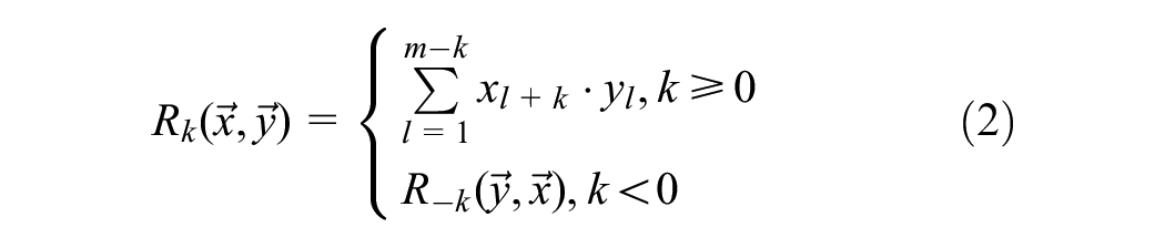
The algorithm is to compute the position w at which $C C_{w} (\vec{x}, \vec{y})$ is maximized. Based on this value of w, the optimal shift of $\vec{x}$ with respect to $\vec{y}$ is then ${\vec{x}}_{(s)}$ , where $s = m - w$ .

Coefficient normalization divides the cross-correlation sequence by the geometric mean of autocorrelations of the individual sequences, defined by Equation 3

{NCC}_{c} (\vec{x}, \vec{y}) = \frac{C C_{w} (\vec{x}, \vec{y})}{\sqrt{R_{0} (\vec{x}, \vec{x}) \cdot R_{0} (\vec{y}, \vec{y})}}

(3)

After normalization of the sequence, the position w where $NC C_{c} (\vec{x}, \vec{y})$ is maximized and the following shape-based distance is derived.

SBD (\vec{x}, \vec{y}) = 1 - max_{w} (\frac{C C_{w} (\vec{x}, \vec{y})}{\sqrt{R_{0} (\vec{x}, \vec{x}) \cdot R_{0} (\vec{y}, \vec{y})}})

(4)

Time-Series Shape Extraction Methods

In this section, the centroid computation is recognized as an optimization where the objective is to find the minimizer of the sum of squared distances to all other time-series sequences. Given a partition $p_{j} \in P$ , the corresponding centroid ${\vec{c}}_{j}$ needs to fulfill Equation 5.

{\vec{c}}_{j} = \underset{\vec{w}}{\arg \min} \sum_{{\vec{x}}_{i} \in p_{j}} {dist (\vec{w}, {\vec{x}}_{i})}^{2}, \vec{w} \in R^{m}

(5)

Shape-Based Time-Series Clustering Methods

The above analysis shows that the K-shape clustering algorithm is developed relying on the shape-based distance measure and shape extraction for centroid computation. In every iteration, K-shape performs two steps: (i) assignment: K-shape updates the cluster members by comparing each time-series with all computed centroids and by assigning each time-series to the cluster of the closest centroid; (ii) refinement: the cluster centroids are updated using the SE method to reflect the changes in cluster memberships in the previous step. The above two steps are repeated until either no change in cluster membership occurs or the set maximum iteration is reached.

Clustering Evaluation Index

To evaluate the clustering performance, two metrics, the Silhouette coefficient (SI) and Calinski-Harabaz index (CI), are calculated by Equations 6 and 7, respectively. Larger values of both SI and CI represent a better clustering performance.

SI (c) = \frac{b - a}{max (a, b)}

(6)

CI (k) = \frac{tr (B_{k})}{tr (W_{k})} \frac{m - k}{k - 1}

(7)

For each cluster c, a represents the average distance from other samples in the same cluster; b represents the average distance from the samples in the closest cluster. m is the number of samples and k is the number of clusters. $B_{k}$ represents the covariance matrix among clusters and $W_{k}$ represents the covariance matrix among samples in the same cluster. Trace of the matrix is denoted as $tr (\cdot)$ .

Data Analysis and Results

Determination of TAZs and Comprehensive Land-Use Patterns

Firstly, taking the longitude and latitude of origin–destination points of online car-hailing services as input, TAZs are determined by clustering. The five typical clustering algorithms discussed in the Methodology section are developed separately. For each clustering algorithm, clustering results are evaluated by adjusting the algorithm parameters and calculating SI. The clustering result with the largest SI is selected as the optimal clustering result, whose cluster numbers and SI are summarized in Table 3.

Table 3.

Optimal Clustering Results of Each Clustering Algorithm

Algorithm	Determination of traffic analysis zones (TAZ)		Land-use determination
Algorithm	Cluster number	Silhouette index (SI)	Cluster number	Silhouette index (SI)
K-means	135	0.352	4	0.346
K-mediods	110	0.483	4	0.162
BIRCH	95	0.425	2	0.338
DBSCAN	70	0.398	6	0.313
Mean-shift	115	0.456	6	0.462

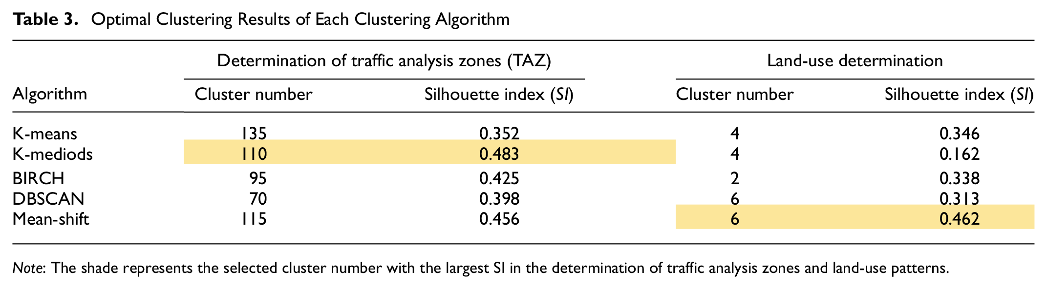
Note: The shade represents the selected cluster number with the largest SI in the determination of traffic analysis zones and land-use patterns.

According to Table 3, different clustering algorithms are further compared based on SI. The K-mediods algorithm, whose cluster number is set to 110, performs best in determining TAZs. Consequently, 110 TAZs are generated by clustering the origin–destination points with the K-mediods algorithm, and the result is shown in Figure 4a. It is found that TAZs located in the central area are smaller than those in the peripheral area. This phenomenon reflects that the central area has a higher land-use intensity and taxi demand.

Figure 4.

(a) Traffic analysis zones (TAZs) determined by K-mediods algorithm in the study area and (b) layout of TAZs matched with comprehensive land-use patterns.

After that, the POI data are matched to the TAZs in which they are located, and the proportion of eight POI categories in each TAZ is computed to reflect the land-use form. The land-use intensity is represented by computing the POI density, which is denoted as the number of POI data per square kilometer. Then, the clustering algorithms are used again to classify the comprehensive land-use patterns by taking the proportion of eight POI categories and land-use density in each TAZ as input. The clustering algorithms are compared again for determining land-use patterns by calculating SI, which is shown in Table 3. Finally, the mean-shift algorithm, whose cluster number is set to six, is selected. Six typical comprehensive land-use patterns are extracted by the mean-shift algorithm, whose layout is shown in Figure 4b. From it, the comprehensive land-use patterns of Type I account for the largest proportion, and the numbers of Type III, Type IV, Type V, and Type VI are small. Analyzed from the geographical location perspective, land-use patterns of Type I and Type II are located in both central and peripheral areas. In contrast, Type III, Type IV, Type V, and Type VI are mainly located in the central areas. Information, including the POI proportion and POI density of each land-use pattern, is shown in Table 4. For ease of understanding the characteristics of each land-use pattern, the visualization is shown in Figure 5.

Table 4.

Typical Patterns Determined by Mean-Shift Algorithm

Pattern	Eating (%)	Shopping (%)	Life service (%)	Health care (%)	Residence (%)	Education (%)	Traffic (%)	Work (%)	Density (/km²)
Type I	20.19	22.75	23.41	7.93	7.81	7.37	2.18	8.36	579.64
Type II	22.06	22.93	23.33	7.22	6.92	7.56	1.45	8.55	1234.78
Type III	26.37	30.07	26.67	5.32	2.54	4.25	0.77	4.01	2231.90
Type IV	13.91	10.39	16.33	2.22	43.11	1.70	9.54	2.81	539.03
Type V	11.98	5.23	7.22	6.10	24.83	17.43	1.60	25.61	1840.02
Type VI	11.70	7.48	13.51	54.40	2.53	6.27	3.62	0.48	502.27

Figure 5.

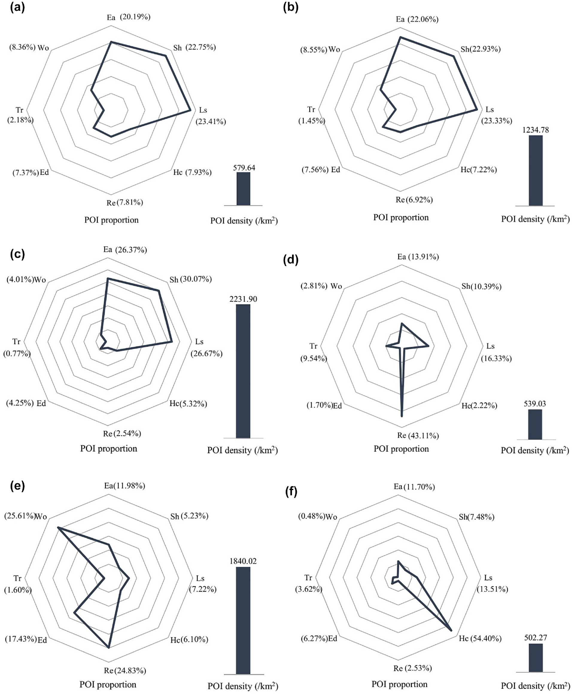
Visualization of characteristics of each land-use pattern: (a) Type I: Low-density commercial district, (b) Type II: Middle-density commercial district, (c) Type III: High-density commercial district, (d) Type IV: Residential district, (e) Type V: Mixed working-living district, and (f) Type VI: Healthcare district.

According to Table 4 and Figure 5, the sum proportion of three land-use forms, Eating, Shopping, and Life service, in Type I, Type II, and Type III is more than 65%, indicating that these three land-use patterns are for commerce. The land-use intensity increases from Type I to Type III. For the convenience of explanation and understanding, land-use patterns of Type I, Type II, and Type III are named Low-density commercial district, Middle-density commercial district, and High-density commercial district, respectively. Residence accounts for a large proportion of the land-use pattern of Type IV, which is named Residential district. The proportion of Transportation in Residential districts is larger than in the other land-use patterns, but the land-use intensity is low. The land-use pattern of Type V is relatively mature, which is named Mixed working-living district. Specifically, Residence, Education, and Work have large proportions in this land-use pattern, where comprehensive services can be obtained. Finally, Health care counts for the largest proportion in the land-use pattern of Type VI, which is named Healthcare district. Compared with other patterns, the land-use intensity in Type VI is the lowest.

From comparison of Low-density commercial district, Middle-density commercial district, and High-density commercial district, the land-use intensity is a determining factor for classifying the land-use patterns when land-use characteristics are identical, indicating the classification of land-use patterns is further refined by introducing land-use intensity in this paper. It is also worth noting that the taxi demand intensity of various land-use categories is differentiated; specifically, points of Traffic and Health care, such as stations and hospitals, have a higher taxi generation and attraction intensity than other land-use categories. Consequently, the land-use intensity is not necessarily consistent with the taxi demand intensity, which should be discussed together with proportions of land-use categories in the following analysis of taxi demand distribution.

Exploration of Taxi Demand Distribution

After the classification of comprehensive land-use patterns, the hourly taxi generation of each TAZ is computed by aggregating the origin points according to the pick-up time, and the hourly taxi attraction of each TAZ is computed by aggregating the destination points according to the drop-off time. Considering that the area of a TAZ affects taxi demand, normalization is made by computing the hourly taxi generation and attraction per square kilometer in each TAZ. For each day, the hourly taxi generation and attraction are transformed into the format of time-series, which is a 24-by-1 matrix. Consequently, a total of 6,380 time-series in 110 TAZs, which reflect hourly taxi generation and attraction, are extracted from 29 days’ records.

Afterward, the K-shape algorithm is developed to extract the typical taxi demand distributions in each comprehensive land-use pattern on weekdays and weekends by taking the time-series of hourly taxi generation and attraction as input. To determine the cluster number in each land-use pattern, the authors set the number of clusters from two to five and compute CI with Equation 7 to evaluate the clustering results. The CI for each cluster number is summarized in Table 5. The final cluster number is set to that with the largest CI, which is highlighted with shade. Finally, the number of set clusters is four for Type I, three for Type II, and two for Types III, IV, V, and VI.

Table 5.

Performance Evaluation of Number of Clusters based on Calinski-Harabaz Index (CI)

Date	Pattern	Number of clusters				Set clusters
Date	Pattern	2	3	4	5	Set clusters
Weekday	Type I	21.16	23.71	39.07	14.75	4
	Type II	6.34	33.25	12.84	14.66	3
	Type III	601.28	311.32	162.28	153.21	2
	Type IV	437.79	199.24	136.99	110.24	2
	Type V	369.70	216.13	114.47	117.20	2
	Type VI	57.94	40.39	18.79	15.69	2
Weekend	Type I	10.78	23.31	30.47	9.05	4
	Type II	24.62	40.57	19.17	10.74	3
	Type III	47.62	25.63	17.56	12.76	2
	Type IV	148.54	111.31	77.78	60.04	2
	Type V	54.53	25.64	20.00	27.97	2
	Type VI	65.98	59.31	54.37	47.35	2

Note: The shade represents the optimal number of clusters with the largest CI for each land-use pattern on weekday and weekend.

With the quantity of clusters determined, the typical distributions of taxi generation and attraction for each land-use pattern on weekdays and weekends are extracted by the K-shape algorithm. The results on weekdays are shown in Figure 6, in which the generation/attraction time is considered according to the pick-up/drop-off time, respectively. Finally, four typical distributions of taxi generation and attraction are extracted in Type I: Low-density commercial district, three typical distributions for Type II: Middle-density commercial district, and two typical distributions for Type III: High-density commercial district, Type IV: Residential district, Type V: Mixed working-living district, and Type VI: Healthcare district.

Figure 6.

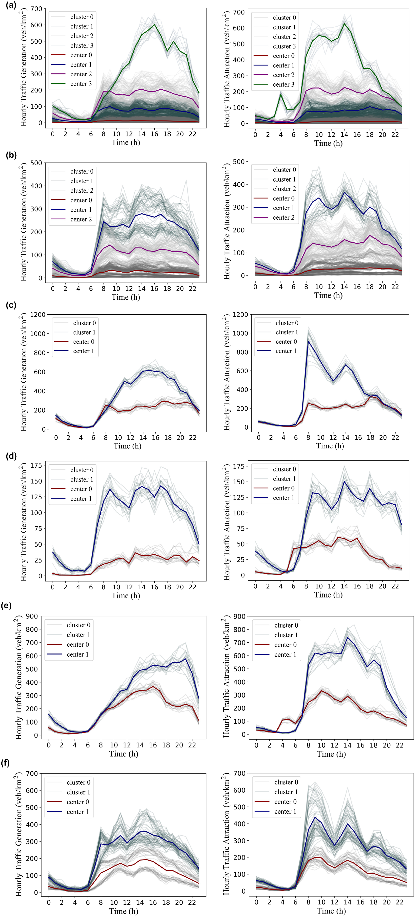
Typical distribution of taxi demand for comprehensive land-use patterns on weekdays: (a-1) Generation—Type I, (a-2) Attraction—Type I, (b-1) Generation—Type II, (b-2) Attraction—Type II, (c-1) Generation—Type III, (c-2) Attraction—Type III, (d-1) Generation—Type IV, (d-2) Attraction—Type IV, (e-1) Generation—Type V, (e-2) Attraction—Type V, (f-1) Generation—Type VI, and (f-2) Attraction—Type VI.

According to taxi generation distribution, taxi generation in each pattern reaches its minimum value at about 5:00 a.m. There is an obvious peak at about 3:00 p.m. in the Low-density commercial district (Type I) and High-density commercial district (Type III), and at about 9:00 p.m. in the Mixed working-living district (Type V). In contrast, there are three traffic peaks at about 8:00 a.m., 2:00 p.m., and 6:00 p.m. in the Residential district (Type IV), which are likely produced by commuter traffic. There is no obvious peak of taxi generation in the Middle-density commercial district (Type II) and Healthcare district (Type VI), meaning taxi generation in the Middle-density commercial district and Healthcare district is more balanced. By comparing different clusters in each pattern, it can be seen that the distribution of taxi generation for different clusters is similar in the Middle-density commercial district, Residential district, and Healthcare district. Nevertheless, in the Low-density commercial district, High-density commercial district, and Mixed working-living district, the cluster with a smaller taxi generation is more balanced, and the traffic peak is more likely to exist for that with a larger taxi generation.

According to the taxi attraction distribution, taxi attraction in each pattern also reaches its minimum value at about 5:00 a.m. Interestingly, a small peak of taxi attraction occurs at about 4:00 a.m. in the Low-density commercial district (Type I) and Mixed working-living district (Type V), which is likely produced by the people who need to start work early, such as breakfast shop staff. Three traffic peaks occur at about 8:00 a.m., 2:00 p.m., and 6:00 p.m. in almost all patterns, except that the traffic peak at about 6:00 p.m. is not obvious in the Low-density commercial district, High-density commercial district, and Healthcare district (Type I, III, and VI, respectively). Comparing different clusters in each pattern, the same conclusion can be drawn as for taxi generation; that is, the clusters with smaller taxi attraction are more balanced, and traffic peaks are more likely to exist for those with larger taxi attraction.

Taxi generation and attraction were then compared, with the finding that their distributions are similar. The distribution of taxi attraction is more concentrated, and taxi attraction is more likely to generate peaks, which is easily seen from comparing taxi generation and attraction in the High-density commercial district (Type III) and Healthcare district (Type VI). This can be explained because the arrival time for work is concentrated, but the departure time is differential because of the different travel distances on weekdays. Considering that Health care accounts for a large proportion in the Healthcare district, a large taxi demand during the two peaks is likely produced by patients and visitors.

The typical distributions of taxi demand for six comprehensive land-use patterns on weekends are also extracted, as Figure 7 shows. The main difference in taxi demand distribution between weekdays and weekends lies in the taxi demand in the morning. On weekends, taxi demand in the morning is reduced and postponed to two hours later. The traffic peaks at 8:00 a.m. on weekdays are missing or cut down on the weekends; instead, the taxi demand after 10:00 a.m. increases. This phenomenon shows that residents would like to rest on weekend mornings, which leads to the delay in travel time. The original traffic peaks on weekdays, which occur at 2:00 p.m. and 6:00 p.m., are also cut down. This indicates that the distribution of taxi generation and taxi attraction becomes more balanced, which can be explained by people’s travel time being more decentralized on weekends.

Figure 7.

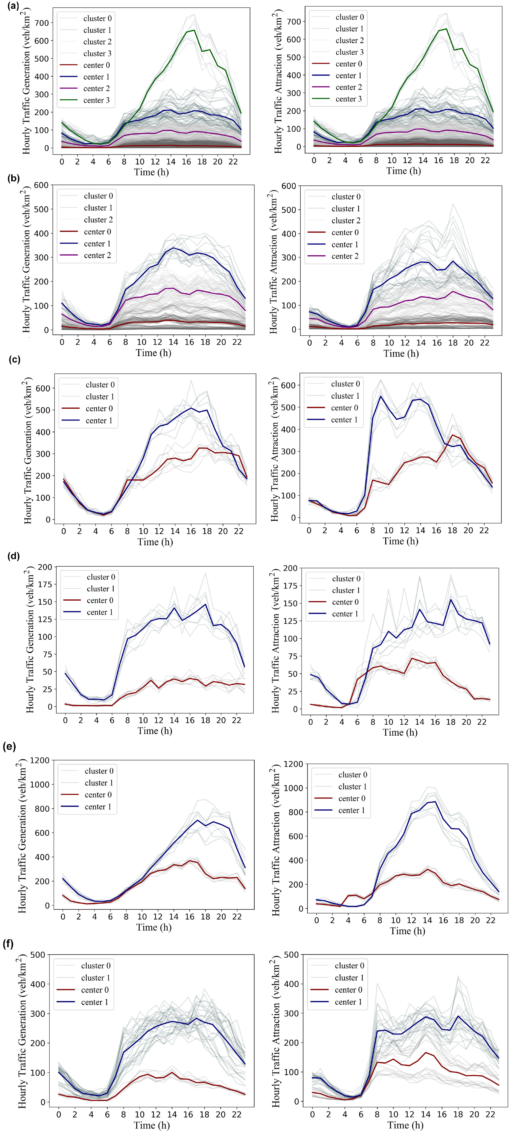
Typical distribution of taxi demand for comprehensive land-use patterns on weekends: (a-1) Generation—Type I, (a-2) Attraction—Type I, (b-1) Generation—Type II, (b-2) Attraction—Type II, (c-1) Generation—Type III, (c-2) Attraction—Type III, (d-1) Generation—Type IV, (d-2) Attraction—Type IV, (e-1) Generation—Type V, (e-2) Attraction—Type V, (f-1) Generation—Type VI, and (f-2) Attraction—Type VI.

Discussion on Taxi Demand Distribution

In this section, typical distributions of taxi demand in each land-use pattern are further analyzed. For each land-use pattern, TTD, denoted as taxi generation plus taxi attraction, and TDD, denoted as taxi attraction minus taxi generation, are computed according to the clustering centers discussed in the previous section. The TTD and TDD of each comprehensive land-use pattern are shown in Figures 8 and 9, respectively. Because the typical taxi generation and taxi attraction are extracted separately according to their time-series characteristic, the overall TDD of each land-use pattern is not exactly equal to zero. The analysis of TDD is focused on the extreme values close to the maximum or minimum, which reflects a significant mismatch between taxi generation and taxi attraction. The average taxi demand of each land-use pattern and hourly taxi demand of each cluster is also counted to reflect the level of dependence on online car-hailing services.

Figure 8.

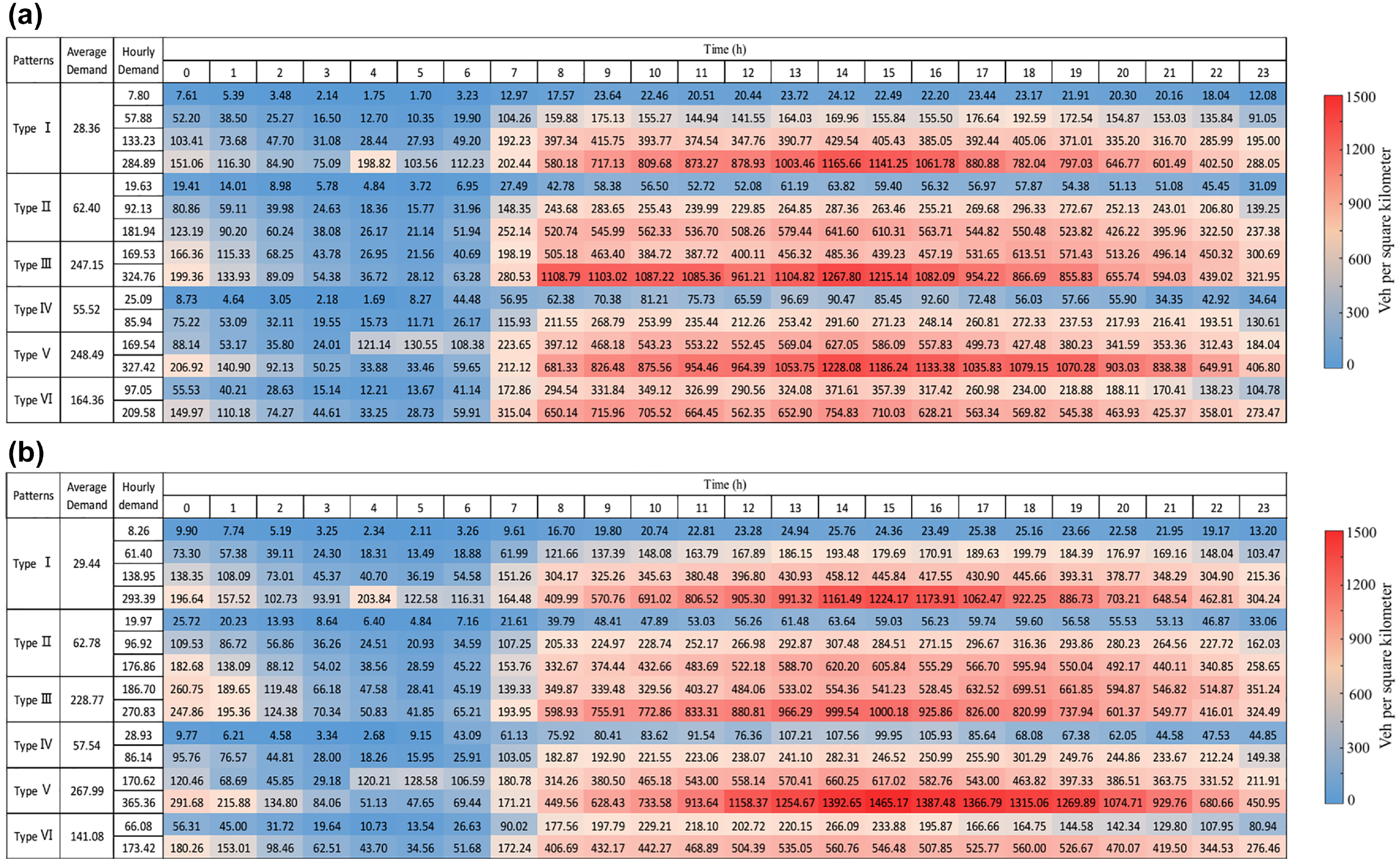
(a) Total taxi demand (TTD) of each comprehensive land-use pattern on weekdays and (b) TTD of each comprehensive land-use pattern on weekends.

Figure 9.

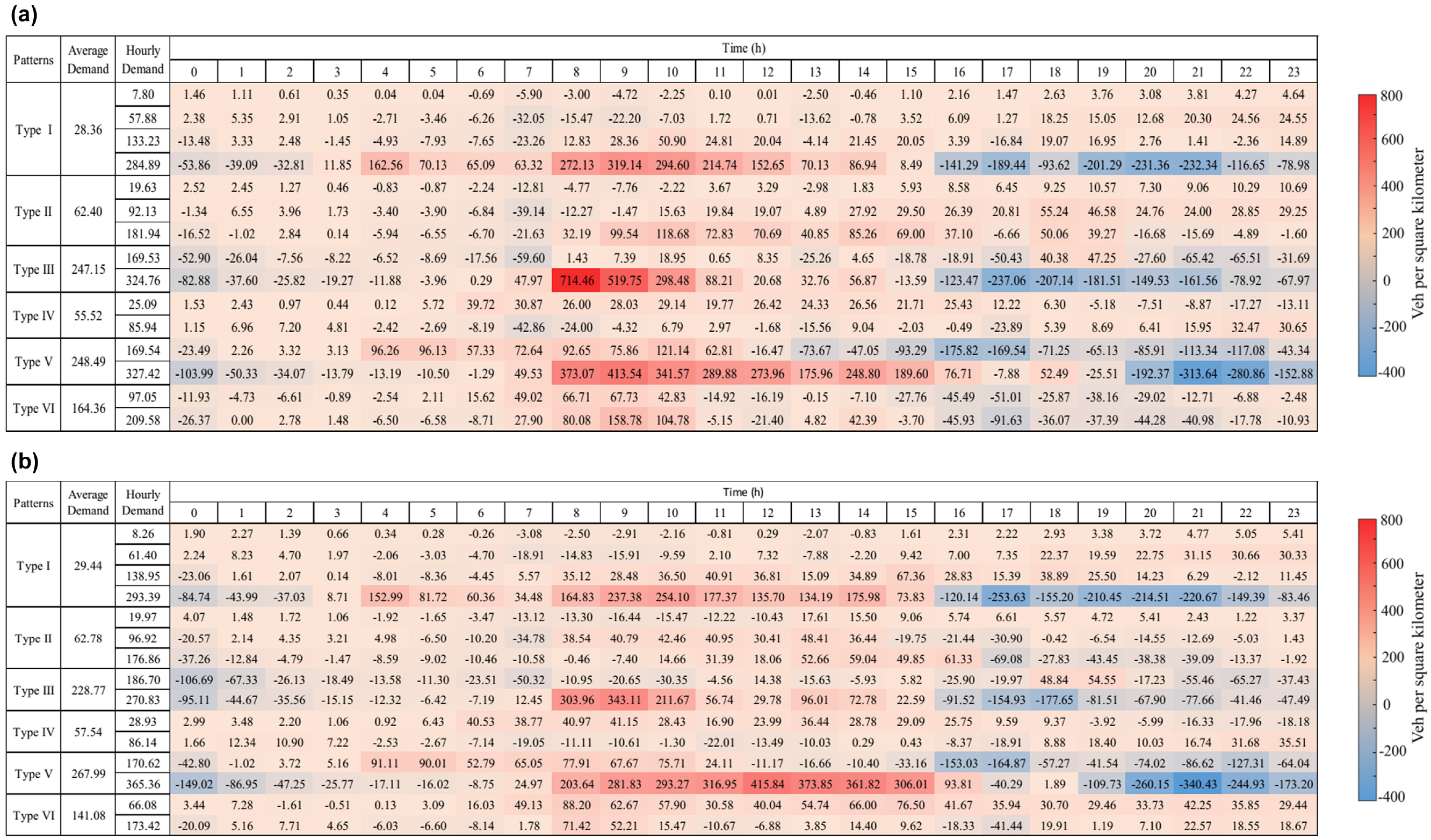
(a) Taxi demand difference (TDD) of each comprehensive land-use pattern on weekdays and (b) TDD of each comprehensive land-use pattern on weekends.

According to Figures 8 and 9, the Mixed working-living district (Type V) has the largest average taxi demand on both weekdays and weekends because of its high land-use intensity and high proportions of Residence, Education, and Work, following by the High-density commercial district (Type III) and Healthcare district (Type VI). By contrast, average taxi demand in the Low-density commercial district, Middle-density commercial district, and Residential district (Type I, II, and IV, respectively) is low. Accordingly, the ranking of dependence on online car-hailing services for different land-use patterns is the Mixed working-living district, High-density commercial district, Healthcare district, Middle-density commercial district, Residential district, Low-density commercial district. It is noted that although the Healthcare district, Low-density commercial district, and Residential district have similar land-use intensity, the average taxi demand in the Healthcare district is larger, indicating the land-use category of Health care is highly dependent on the online car-hailing service.

TTD reflects the overall taxi demand in an area, and a larger TTD represents a higher taxi demand intensity. From the TTD of each land-use pattern shown in Figure 8, high TTD mainly concentrates from 8:00 a.m. to 10:00 p.m. on weekdays and 9:00 a.m. to 10:00 p.m. on weekends. The dependence level of online car-hailing services is high and traffic management for taxis should be strengthened in the following three situations: (i) Low-density commercial district (Type I) whose hourly taxi demand reaches about 285 veh/km², (ii) High-density commercial district (Type III) whose hourly taxi demand reaches about 325 veh/km², (iii) Mixed working-living district (Type V) whose hourly taxi demand reaches about 350 veh/km². During weekends, the high TTD of the above situation (ii) is reduced, while the TTD of the above situation (iii) enlarges, especially from midday to 7:00 p.m.

TDD in Figure 9 reflects the difference between taxi generation and taxi attraction. When TDD is too large or too small, taxi demand is not balanced, leading to waste of resources in the taxi system. From the TDD of each land-use pattern, similar to the distribution of TTD, TDD of the above three situations also has characteristics that are obviously tidal. The high TDD is mainly concentrated on the period from 8:00 a.m. to 3:00 p.m., while the low TDD is mainly concentrated on the evening period from 4:00 to 11:00 p.m. TTD reaches a high value in the above situations (ii) and (iii) from 8:00 to 10:00 a.m. on weekdays. The large TTD in situation (ii) is reduced on weekends, but that in situation (iii) is postponed from midday to 2:00 p.m. The low TTD in situation (iii) is concentrated on the period from 8:00 to 11:00 p.m., which represents a few hours’ delay compared with the other situations.

Furthermore, the average hourly origin–destination matrix between each land-use pattern on weekdays and weekends is shown in Figure 10. By comparing Figure10a with Figure10b, it can be seen that taxi demand in the Mixed working-living district (Type V) is increased, and that in the Healthcare district (Type VI) and High-density commercial district (Type III) is decreased on weekends compared with weekdays. Taxi demand on other land-use patterns is not obviously different between weekdays and weekends. Further analyzing the taxi demand of different land-use patterns, the Mixed working-living district (Type V) and High-density commercial district (Type III) have a larger taxi demand than other land-use patterns. Taxi demand in the land-use patterns of Low-density commercial district, Middle-density commercial district, and Residential district (Type I, II, and IV, respectively) remains at a low level on both weekdays and weekends. Taxi demand in the Mixed working-living district (Type V) and High-density commercial district (Type III) is the largest, indicating that these two land-use patterns are closely related.

Figure 10.

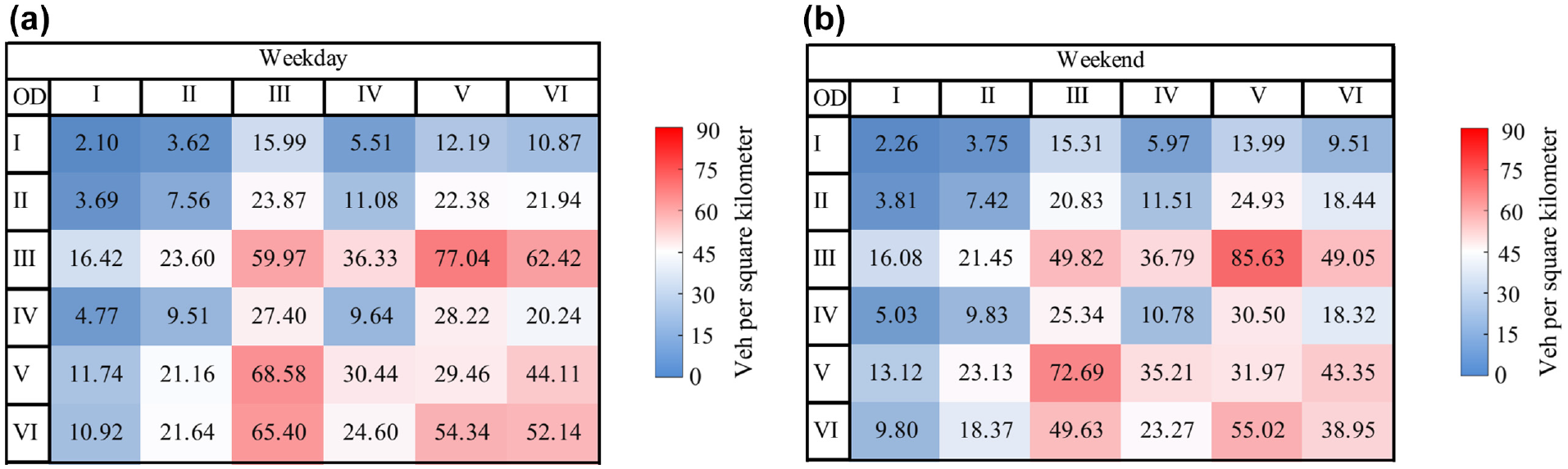
(a) Average hourly origin–destination (OD) matrix of taxis between land-use patterns on weekdays and (b) Average hourly OD matrix of taxis between land-use patterns on weekends.

Combining the above analyses, some conclusions and suggestions are drawn on the three aspects of traffic management, land-use combination, and land-use adjustment.

Traffic management: (a) traffic management authorities could allocate more traffic resources and optimize traffic organization in the Low-density commercial district, High-density commercial district, and Mixed working-living district (Type I, III, and V, respectively), where average hourly taxi demand reaches about 300 veh/km². Some management measures, including traffic restriction, congestion charging, and signal optimization, can be preferentially considered to be set around these land-use patterns to receive the heavy taxi demand. (b) Differential traffic management should be set up on weekdays and weekends. The concentrated taxi demand in the High-density commercial district (Type III) is relieved on weekends. Accordingly, it is reasonable to transfer partial traffic resources in the High-density commercial district to other patterns which have increased taxi demand on weekends, such as the Mixed working-living district (Type V).

Land-use combination: (a) Middle-density commercial districts (Type II) are suited to form a combination with the Mixed working-living district (Type V) or Healthcare district (Type VI) considering their TDD is complementary. Redundant taxis, having arrived in the Mixed working-living district and Healthcare district, could undertake some taxi generation in the Middle-density commercial districts from 8:00 to 10:00 a.m., avoiding the no-load running of taxis and reducing energy consumption. (b) When carrying out land-use planning, High-density commercial district (Type III) and Mixed working-living district (Type V) should not be adjacent to each other, to avoid excessive concentration of taxi demand. A Healthcare district (Type VI) should be set in the central area around other land-use patterns to reduce the travel distance and provide convenience for medical services.

Land-use adjustment: (a) TDD in the high-density commercial district (Type III) is more concentrated than in the Mixed working-living district (Type V), indicating that the mixed land-use patterns are beneficial for relieving the mismatch of TDD. Consequently, the commercial district can be adjusted by merging into other land-use categories, such as Residence, to avoid unbalanced TDD. (b) The mismatch of TDD is aggravated by the increased hourly taxi demand in each land-use pattern, indicating that reasonably limiting the concentration of land-use categories that are highly dependent on taxis, such as Health care and Traffic, is necessary for land-use planning.

Conclusion

This study explores the taxi demand distribution of comprehensive land-use patterns using online car-hailing data and POI data in Chengdu, China. Origin–destination points are extracted from the online car-hailing data, and 110 TAZs are generated by clustering origin–destination points with the K-mediods algorithm. Then POI data is matched with each TAZ to compute the proportion of land-use forms and land-use intensity. Six typical comprehensive land-use patterns are determined using the mean-shift algorithm. By transforming the hourly taxi demand into the format of time-series, the K-shape algorithm is developed to extract the typical taxi demand distributions of taxi generation and attraction in each pattern. Finally, TTD and TDD are computed to reflect taxi demand distribution and provide accurate guidance for traffic control.

From the process of exploring the taxi demand distribution, the following conclusions are made: (i) six typical comprehensive land-use patterns are determined in Chengdu, and the land-use intensity plays an important role in the determination of land-use patterns; (ii) even under the same comprehensive land-use pattern, traffic taxi distributions are still differentiated. When the taxi demand is higher, taxi demand distribution is more unbalanced, and obvious traffic peaks are more likely to generate. The findings of this study can provide suggestions for traffic management, land-use combination, and land-use adjustment to avoid concentrated taxi demand and mismatched taxi generation/attraction, specifically: (i) traffic management should be mainly made on the Low-density commercial district, High-density commercial district, and Mixed working-living district, whose the average hourly taxi demand reaching about 300 veh/km², with differentiated schemes on weekdays and weekends; (ii) Middle-density commercial districts are suited to form a combination with the Mixed working-living district or Healthcare district, but High-density commercial district and Mixed working-living district should be not adjacent; (iii) mixing multiple land-use categories and limiting the concentration of land-use categories which are highly dependent on taxis is beneficial for relieving the mismatched taxi generation/attraction.

Some limitations still exist in this study. First, the traffic demand reflected by online car-hailing data mainly concentrates on Chengdu’s central area, where the land-use forms are extremely similar. This phenomenon results in the imbalance of the quantity of various comprehensive land-use patterns. Besides, with its limitation to online car-hailing data, this study only analyzes the taxi demand in Chengdu, which would limit the applicability of the findings. In the future, more online car-hailing datasets from additional cities and other types of travel datasets, such as the RFID dataset and mobile phone signaling dataset, can be used for testing the findings of this study and analyzing the traffic demand of other modes to expand the applicability of this research.

Footnotes

Author Contributions

The authors confirm contribution to the paper as follows: study conception and design: Xuedong Hua and Wei Wang; data collection: Weijie Yu, and Xueyan Wei; analysis and interpretation of results: Weijie Yu and Xuedong Hua; draft manuscript preparation: Weijie Yu, Xuedong and Wei Wang. All authors reviewed the results and approved the final version of the manuscript.

Declaration of Conflicting Interests

The author(s) declared no potential conflicts of interest with respect to the research, authorship, and/or publication of this article.

Funding

The author(s) disclosed receipt of the following financial support for the research, authorship, and/or publication of this article: The research is supported by the National Natural Science of China (71801042, 51878166) and the Natural Science of Jiangsu Province (BK20180381).

Data Availability Statement

Data source: Didi Chuxing GAIA Initiative.

References

Fang

Wang

Quantitative Diagnoses and Comprehensive Evaluations of the Rationality of Chinese Urban Development Patterns. Sustainability, Vol. 7, No. 4, 2015, pp. 3859–3884.

Alalouch

Al-Hajri

Naser

Hinai

A. A.

The Impact of Space Syntax Spatial Attributes on Urban Land Use in Muscat: Implications for Urban Sustainability. Sustainable Cities and Society, Vol. 46, 2019, p. 101417.

Lee

J.-S.

Nam

Lee

S.-S.

Built Environment Impacts on Individual Mode Choice: An Empirical Study of the Houston-Galveston Metropolitan Area. International Journal of Sustainable Transportation, Vol. 8, No. 6, 2014, pp. 447–470.

Wei

Zuo

Liu

Yang

Y. J.

Integrating Land Use and Socioeconomic Factors into Pattern-Based Travel Demand and Carbon Emission Impact Study. Urban Rail Transit, Vol. 3, No. 1, 2017, pp. 3–14.

Radhakrishnan

Aswathy

Mathew

Studying Land Use Travel Demand Interaction Using 3S Technology for Tiruchirappalli City. Journal of the Indian Society of Remote Sensing, Vol. 45, No. 5, 2017, pp. 815–824.

Zhou

Kockelman

K. M.

Lemp

J. D.

Applications of Integrated Transport and Gravity-Based Land Use Models for Policy Analysis. Transportation Research Record: Journal of the Transportation Research Board, 2009. 2133: 123–132.

Wagner

Regional Traffic Impacts of Logistics-Related Land Use. Transport Policy, Vol. 17, No. 4, 2010, pp. 224–229.

Gao

Wang

Liu

Wang

Zhang

Travel Behavior Analysis Using 2016 Qingdao’s Household Traffic Surveys and Baidu Electric Map API Data. Journal of Advanced Transportation, Vol. 2019, 2019, pp. 1–18.

Currans

K. M.

Clifton

K. J.

Using Household Travel Surveys to Adjust ITE Trip Generation Rates. Journal of Transport and Land Use, Vol. 8, No. 1, 2015, pp. 85–119.

10.

Zhou

Qian

Xiao

Xin

Wei

Feng

Coupling Research on Land Use and Travel Behaviors along the Tram Based on Accessibility Measurement—Taking Nanjing Chilin Tram Line 1 as an Example. Sustainability, Vol. 11, No. 7, 2019, p. 2034.

11.

Salon

Heterogeneity in the Relationship between the Built Environment and Driving: Focus on Neighborhood Type and Travel Purpose. Research in Transportation Economics, Vol. 52, 2015, pp. 34–45.

12.

Tang

Wang

Assessing Intercity Multimodal Choice Behavior in a Touristy City: A Factor Analysis. Journal of Transport Geography, Vol. 86, 2020, p. 102776.

13.

Bao

Liu

Wang

Exploring Bikesharing Travel Patterns and Trip Purposes Using Smart Card Data and Online Point of Interests. Networks and Spatial Economics, Vol. 17, No. 4, 2017, pp. 1231–1253.

14.

Xiang

Wang

Hua

Wang

Investigating Dominant Trip Distance for Intercity Passenger Transport Mode Using Large-Scale Location-Based Service Data. Sustainability, Vol. 11, No. 19, 2019, p. 5325.

15.

Liu

Kang

Gao

Xiao

Tian

Understanding Intra-Urban Trip Patterns from Taxi Trajectory Data. Journal of Geographical Systems, Vol. 14, No. 4, 2012, pp. 463–483.

16.

Niu

Zhu

Zhang

DeepSense: A Novel Learning Mechanism for Traffic Prediction with Taxi GPS Traces. Proc., 2014 IEEE Global Communications Conference, Austin, TX, IEEE, New York, 2014, pp. 2745–2750.

17.

Heilmann

Faouzi

N.-E. E.

de Mouzon

Hainitz

Koller

Bauer

Antoniou

Predicting Motorway Traffic Performance by Data Fusion of Local Sensor Data and Electronic Toll Collection Data. Computer-Aided Civil and Infrastructure Engineering, Vol. 26, No. 6, 2011, pp. 451–463.

18.

Pouke

Goncalves

Ferreira

Kostakos

Practical Simulation of Virtual Crowds Using Points of Interest. Computers, Environment and Urban Systems, Vol. 57, 2016, pp. 118–129.

19.

Marchal

A Trip Generation Method for Time-Dependent Large-Scale Simulations of Transport and Land-Use. Networks and Spatial Economics, Vol. 5, No. 2, 2005, pp. 179–192.

20.

Lin

J.-J.

Yang

A. T.

Structural Analysis of How Urban Form Impacts Travel Demand: Evidence from Taipei. Urban Studies, Vol. 46, No. 9, 2009, pp. 1951–1967.

21.

Wang

Han

de Vries

Land Use/Land Cover and Accessibility: Implications of the Correlations for Land Use and Transport Planning. Applied Spatial Analysis and Policy, Vol. 12, No. 4, 2019, pp. 923–940.

22.

Wang

Sun

Identification of Urban Functional Regions Based on Floating Car Track Data and Poi Data. Sustainability, Vol. 11, No. 23, 2019, p. 6541.

23.

Viegas

J. M.

Martínez

L. M.

Silva

E. A.

Effects of the Modifiable Areal Unit Problem on the Delineation of Traffic Analysis Zones. Environment and Planning B: Planning and Design, Vol. 36, No. 4, 2009, pp. 625–643.

24.

Pani

Sahu

P. K.

Chandra

Sarkar

A. K.

Assessing the Extent of Modifiable Areal Unit Problem in Modelling Freight (Trip) Generation: Relationship between Zone Design and Model Estimation Results. Journal of Transport Geography, Vol. 80, 2019, p. 102524.

25.

Altan

M. F.

Ayözen

Y. E.

The Effect of the Size of Traffic Analysis Zones on the Quality of Transport Demand Forecasts and Travel Assignments. Periodica Polytechnica-Civil Engineering, Vol. 62, No. 4, 2018, pp. 971–979.

26.

Liu

Yan

Wang

Yang

Grid Mapping for Spatial Pattern Analyses of Recurrent Urban Traffic Congestion Based on Taxi GPS Sensing Data. Sustainability, Vol. 9, No. 4, 2017, p. 533.

27.

Wang

Taxi Driver’s Operation Behavior and Passengers’ Demand Analysis Based on GPS Data. Journal of Advanced Transportation, Vol. 2018, 2018, pp. 1–11.

28.

Yang

Sun

Shang

Wang

Zhu

Understanding Collective Human Mobility Spatiotemporal Patterns on Weekdays from Taxi Origin-Destination Point Data. Sensors, Vol. 19, No. 12, 2019, p. 2812.

29.

Shen

Liu

Chen

Discovering Spatial and Temporal Patterns from Taxi-Based Floating Car Data: A Case Study from Nanjing. GIScience & Remote Sensing, Vol. 54, No. 5, 2017, pp. 617–638.

30.

Sun

Ling

Tan

Community Structure in Traffic Zones Based on Travel Demand. Physica A-Statistical Mechanics and its Applications, Vol. 457, 2016, pp. 356–363.

31.

Hochmair

H. H.

Spatiotemporal Pattern Analysis of Taxi Trips in New York City. Transportation Research Record: Journal of the Transportation Research Board, 2016. 2542: 45–56.

32.

Chen

Network-Wide Identification of Turn-Level Intersection Congestion Using only Low-Frequency Probe Vehicle Data. Transportation Research Part C-Emerging Technologies, Vol. 108, 2019, pp. 320–339.

33.

Zhang

Sun

Shen

Zhu

Analyzing Spatiotemporal Congestion Pattern on Urban Roads Based on Taxi GPS Data. Journal of Transport and Land Use, Vol. 10, No. 1. 2017, pp. 675–694.

34.

Tulic

Bauer

Scherrer

Link and Route Travel Time Prediction Including the Corresponding Reliability in an Urban Network Based on Taxi Floating Car Data. Transportation Research Record: Journal of the Transportation Research Board, 2014. 2442: 140–149.

35.

Markou

Rodrigues

Pereira

F. C.

Demand Pattern Analysis of Taxi Trip Data for Anomalies Detection and Explanation. Transportation Research Record: Journal of the Transportation Research Board, 2017. 2643: 129–138.

36.

Yang

Gonzales

E. J.

Modeling Taxi Trip Demand by Time of Day in New York City. Transportation Research Record: Journal of the Transportation Research Board, 2014. 2429: 110–120.

37.

Murtagh

Contreras

Algorithms for Hierarchical Clustering: An Overview. Wiley Interdisciplinary Reviews-Data Mining and Knowledge Discovery, Vol. 2, No. 1, 2012, pp. 86–97.

38.

Paparrizos

Gravano

Fast and Accurate Time-Series Clustering. ACM Transactions on Database Systems (TODS), Vol. 42, No. 2, 2017, p. 8.

39.

Jarabek

Laurinec

Lucka

Energy Load Forecast Using S2S Deep Neural Networks with k-Shape Clustering. Proc., 2017 IEEE 14th International Scientific Conference on Informatics, Poprad, Slovakia, IEEE, New York, 2017, pp. 140–145.