Analysis of Headway and Speed Based on Driver Characteristics and Work Zone Configurations Using Naturalistic Driving Study Data

Abstract

The objective of this paper is to analyze headway and speed distribution based on driver characteristics and work zone (WZ) configurations by utilizing Naturalistic Driving Study (NDS) data. The NDS database provides a unique opportunity to study car-following behaviors for different driver types in various WZ configurations, which cannot be achieved from traditional field data collection. The complete NDS WZ trip data of 200 traversals and 103 individuals, including time-series data, forward-view videos, radar data, and driver characteristics, was collected at four WZ configurations, which encompasses nearly 1,100 vehicle miles traveled, 19 vehicle hours driven, and over 675,000 data points at 0.1 s intervals. First, the time headway selections were analyzed with driver characteristics such as the driver’s gender, age group, and risk perceptions to develop the headway selection table. Further, the speed profiles for different WZ configurations were established to explore the speed distribution and speed change. The best-fitted curves of time headway and speed distributions were estimated by the generalized additive model (GAM). The change point detection method was used to identify where significant changes in mean and variance of speeds occur. The results concluded that NDS data can be used to improve car-following models at WZs that have been implemented in current WZ planning and simulation tools by considering different headway distributions based on driver characteristics and their speed profiles while traversing the entire WZ.

The number of work zones (WZs) has been increasing in the U.S.A. to address the growing needs for highway maintenance and construction as the National Highway System is aging. According to the Federal Highway Administration (FHWA), WZs accounted for an estimated 10% of overall congestion and 24% of unexpected freeway delays, which was equivalent to about 888 million vehicle hours in 2014 ( 1 ). Reduced operating speeds, narrowed lane widths, and smaller shoulder clearances cause the capacity per lane in WZ to be lower than non-WZ sections ( 2 ). Thus, to facilitate the highway construction work and mitigate the delay issues, the state Departments of Transportation (DOT) and local transportation agencies have applied various simulation models and planning tools to estimate or predict WZ capacity ( 2 – 8 ). Traffic simulation software, for example, CORSIM (University of Florida, U.S.A.) and VISSIM (Karlsruhe, Germany), have been used for decades to estimate the operational capacity of WZs with different configurations ( 7 , 9 , 10 ). The calibration of these simulation models requires quite an amount of field data to ensure the accuracy of the estimated results. Meanwhile, the planning-level WZ simulation tools such as QUEWZ (University of Florida) and QuickZone (FHWA) are also popular among DOTs, although it has been reported that QUEWZ and QuickZone were inaccurate because of outdated field data and parameters ( 11 – 14 ).

The second Strategic Highway Research Program (SHRP2) Naturalistic Driving Study (NDS) has shown the potential to provide various data which can be used to refine the estimated results from these models and tools. The SHRP2 NDS data is a new approach to investigate driver behavior during daily trips through unobtrusive data-gathering equipment and without experimental control ( 15 ). Compared with traditional field data collection techniques, the NDS database offers a unique opportunity to observe actual WZ layouts, traffic conditions, and driver performance while negotiating freeway WZs ( 16 ). In a previous study, the researchers utilized the NDS data to evaluate capacity, car-following characteristics, and driver types in three freeway WZ configurations: two-to-one lane closure (LC 2-1), two-to-two shoulder closure (SC 2-2), and three-to-three shoulder closure (SC 3-3) ( 17 ). That was the first study to apply NDS data to study headway distribution at WZs based on driver characteristics. Because of the limited sample size, it recommended collecting more complete trip data, that is, from vehicles traversing the entire WZ (500 ft upstream, advance warning area, transition area, activity area, termination area, and 500 ft downstream) for further study. Thus, in this study, the objectives were set: (i) to develop time headway selection tables based on different driver characteristics (i.e., gender, age group, and risk perception) at four WZ configurations; (ii) to compare the headway distributions at different consecutive WZ sections; and (iii) to perform an analysis of speed to explore the speed distribution and speed change at WZs.

Literature Review

A thorough literature review was conducted to assess the state of the practice in WZ headway distribution, speed studies, and existing NDS applications.

Headway Distribution

Vehicle time headway is a critical traffic flow characteristic that affects the level of service and capacity ( 18 ). Thus, it is of utmost importance to analyze this factor in relation to WZs, so that the accurate vehicle dynamics in WZs can be generated. Headway distribution modeling has been studied for decades ( 19 ). Many vehicle headway distribution models have been proposed to model the vehicle headway at various traffic flow levels, including exponential distribution, Weibull distribution, gamma distribution, lognormal distribution, Erlang distribution, and inverse Gaussian distribution ( 20 – 22 ). These studies only fit the models in mixed vehicular traffic without consideration of vehicle headways for different types of vehicle-following patterns. Thus, some researchers have begun to disaggregate vehicle headways into various types of leader-and-follower vehicle pairs, such as the car-truck pair, truck-car pair, truck-truck pair, and car-car pair ( 19 , 23 , 24 ). However, as WZ traffic has unique characteristics, few studies have explored vehicle headway distribution in WZs ( 21 , 24 ). Moreover, none of the existing studies took into account the effects of driver characteristics on headway in WZs, despite different drivers exhibiting various influences that contribute to their unique driving behaviors. Therefore, there is a need to develop headway selection tables based on driver characteristics in WZs.

Speed Studies

Previous studies of speed in WZs mainly addressed factors affecting speed limits, driver compliance with speed limits, enforcement, and safety issues ( 25 – 31 ). As recommended by the National Cooperative Highway Research Program (NCHRP), the normal posted speed is typically reduced by 10 mph when called for ( 25 ). Changeable message sign (CMS), speed display trailers or CMS with radar, innovative signs, flagging treatments, lane narrowing, late merge, transverse striping, and rumble strips are the commonly used speed reduction methods and strategies in WZs ( 26 – 28 ). For driver compliance, it was found that compliance was the greatest where the speed limit was not reduced, and compliance decreased where the speed limit was reduced by 10 mph more ( 29 ). Enforcement tools typically refer to police vehicle patrolling or a speed feedback trailer. However, research has shown that once the enforcement tool is out of sight, vehicle speeds return to their previous levels ( 30 ). As for safety issues, it was revealed that the greatest number of fatal crashes occurred on highways with speed limits between 65 and 70 mph, which confirmed that high speeds increase the severity of WZ crashes ( 31 ). Furthermore, the previous studies of speed in WZs utilized spot-measured data, which failed to provide a full picture of speed profiles. Thus, it would be useful to perform a speed analysis that explores the speed distribution and speed change in the form of time series at WZs.

Existing NDS Applications

SHRP2 NDS data involves 3,147 drivers collected from 2010 to 2012 in six states: New York, Pennsylvania, Florida, Washington, North Carolina, and Indiana ( 16 ). SHRP2 was targeted on addressing the role of driver performance and behavior in traffic safety and understanding how the driver interacts with and adapts to the vehicle, environmental conditions, roadway geometric characteristics, and traffic control devices ( 32 ). Thus, most studies that utilize NDS data mainly focus on traffic safety, while some pay attention to the impacts of roadway geometric design features ( 33 – 35 ). The focus of existing WZ studies that utilize NDS data is predominantly on safety analysis, and very few have aimed to explore the headway distribution based on driver characteristics ( 17 , 36 – 38 ).

In summary, the review of the available literature indicated that very few WZ studies in the past considered driver characteristics and their car-following behaviors. The NDS data can provide this unique information that could not be obtained from field data collection or simulation models in the past. The driver types and their headway distributions in WZ would be helpful to identify how driver behaviors affect WZ capacity. Based on the literature review results, this is the first study to apply NDS data to study the impact of driver characteristics on headway selection and speed distribution during the entire WZ areas. Furthermore, the results can be used to enhance WZ planning and simulation models by considering different headway distributions based on driver characteristics and their speed profiles traversing the entire WZ.

Methods

Data Collection and Reduction

A conference call was scheduled with Virginia Tech Transportation Institute (VTTI) staff to request the appropriate NDS data on WZs. First, over 58 h of sample video clips were delivered to identify WZ start and end mileposts, so that the trips traversing the same locations during the same time periods could be exported. The exported time interval covers at most 20 weeks (10 weeks before and 10 weeks after the identified sample trips occurred). However, as WZ activity proceeds, the configuration changes very quickly. For example, although WZ start and end mileposts were identified from the first step, the WZ configuration might have changed within two weeks (one week before and one week after the identified sample trips). Thus, all the NDS videos received were reviewed to ensure that they were categorized into the proper WZ configuration.

Time-series data (i.e., speed), radar data (i.e., time headway), and video clips of the forward roadway were obtained for each trip. All the time-series data and radar data were collected at 0.1 s intervals. From the radar data dictionary file, the headway is equal to the distance between target and participant vehicle’s front bumper divided by the participant’s vehicle speed. The video can also be linked to time-series data and radar data so that the corresponding speed and time headway at certain 0.1 s can be acquired. Driver risk perception and driver demographics were also requested. Driver risk perceptions were calculated based on self-reported measures, which indicated their perceptions of risk associated with different driving behaviors. The scores range from 32 to 224. Higher scores indicate greater risk perceptions; therefore, these drivers self-reported as cautious and obedient to traffic rules. The driver risk perception was collected from the questionnaire designed to gauge the participant’s perception of dangerous or unsafe driving behaviors or scenarios ( 39 ). This questionnaire includes 32 driving-behavior-related questions. For example, how would the participant evaluate the risk when not yielding the right of way; the risk the participant associated with passing other cars on the right side or the shoulder of the road, the risk the participant associated with turning without signaling, and so forth. Each question was assigned a score from 1 (No Greater Risk) to 7 (Much Greater Risk); thus, a higher score indicates that the driver is more cautious or obedient to traffic rules. The total risk perception score of drivers is the sum of all the scores from questions in the questionnaire.

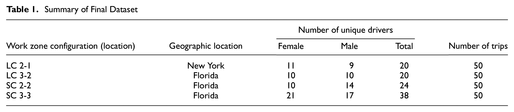
To eliminate potential distraction or impact from non-WZ elements, only trips that occurred during daylight time with clear vision in good weather conditions on dry pavement were selected. To reduce the impact of interchanges near WZs that might potentially influence driver performance, trips affected by interchanges within WZs were also filtered out to exclude the effects of merging and diverging maneuvers by participating drivers or/and surrounding drivers. Finally, 200 complete WZ trips that traversed the entire WZ (500 ft upstream, advance warning area, transition area, activity area, termination area, and 500 ft downstream) driven by 103 unique drivers from four WZ locations representing four configurations were selected. According to FHWA, lane closure and shoulder closure are the most common types of construction in WZs ( 40 ). Meanwhile, four- and six-lane divided highways are the most common types of roadways in the Interstate system, occupying over 90% of the mileage ( 41 ). Thus, four WZ configurations were selected in this study as presented in Figure 1. They are lane closure with lane reduction from two lanes to one lane (LC 2-1), lane closure with lane reduction from three lanes to two lanes (LC 3-2), shoulder closure with two lanes (SC 2-2), and shoulder closure with three lanes (SC 3-3), which encompass nearly 1,100 vehicle miles traveled, 19 vehicle hours driven, and over 675,000 data points at 0.1 s intervals. All WZ configurations complied with the requirements of Temporary Traffic Control zones in the Manual on Uniform Traffic Control Devices ( 42 ). The speed control methods were only applied at lane closure configurations with portable changeable message signs at the beginning of transition area. WZ speed limits that affect speed choice only appeared in the LC 2-1 locations. There was no other law enforcement to affect speed reduction in the other three WZ locations. Only SC 2-2 had concrete barriers while the other three WZ configurations all used drums. Table 1 summarizes numbers of unique drivers and trips at each WZ configuration (location), and their geographic locations. One LC 2-1 WZ is located in New York State, and the other three WZs are located in Florida.

Figure 1.

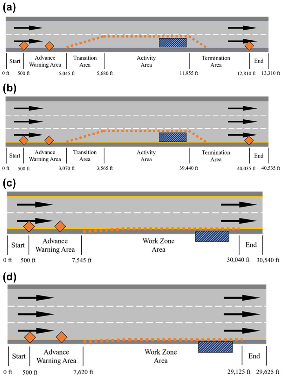
Four work zone (WZ) configurations: (a) LC 2-1, (b) LC 3-2, (c) SC 2-2, and (d) SC 3-3.

Table 1.

Summary of Final Dataset

Work zone configuration (location)	Geographic location	Number of unique drivers			Number of trips
Work zone configuration (location)	Geographic location	Female	Male	Total	Number of trips
LC 2-1	New York	11	9	20	50
LC 3-2	Florida	10	10	20	50
SC 2-2	Florida	10	14	24	50
SC 3-3	Florida	21	17	38	50

Headway Distribution

The time headway distributions in the freeway WZs were explored under different WZ configurations. Time headway is defined as the time between two consecutive vehicles (in seconds) when they pass a single point on a roadway ( 43 ). A WZ typically consists of four consecutive sections: advance warning area, transition area, activity area, and termination area. In lane closure WZs (Figure 1, a and b ), it is easy to define these four sections. But in shoulder closure WZs (Figure 1, c and d ), the borders of transition area, activity area, and termination area are not clear. Thus, only three areas were defined for shoulder closure WZs as: WZ area, 500 ft upstream and downstream of WZs to measure the driver behavior changes before and after WZs.

To identify the relationships between headway selection and driver characteristics, male and female drivers were categorized into young, middle-aged, and senior groups. The driver’s mean time headway, its 95% confidence interval, and the associated risk score were investigated. Further analysis was conducted to find out drivers’ headway changes through the entire WZ.

Generalized Additive Model

To explore the driver’s headway distribution through the entire WZ, the generalized additive model (GAM) was used to predict the best-fitted curve of headway profile of WZ consecutive sections to provide a better understanding of how drivers negotiated the entire WZ, given the headway data from NDS. GAM is a powerful and yet simple technique. When compared with other techniques, GAM has three key advantages: (i) easy to interpret; (ii) flexible predictor functions can uncover hidden patterns in the data; and (iii) regularization of predictor functions helps avoid overfitting ( 44 ). GAM ( 45 , 46 ) allows non-linear functions of each variable, while maintaining the additivity of the model. This is achieved by replacing each linear component β_jx_ij by a smooth non-linear function f_j(x_ij). A GAM can be written as Equation 1:

\begin{matrix} y_{i} = β_{0} + \sum_{j = 1}^{n} f_{j} (x_{ij}) + ε_{i} = β_{0} + f_{1} (x_{i 1}) + f_{2} (x_{i 2}) + \dots + f_{n} (x_{in}) + ε_{i} \end{matrix}

(1)

where $y_{i}$ is the dependent variable, $x_{in}$ is the predictor variable, and $f_{n} (x_{in})$ is the smooth non-linear function.

GAM allows fitting a non-linear function f_j to each x_j so that one does not need to manually try out numerous transformations on each of the predictor variables. Since GAM is an additive model, one can examine the impact of each x_j on y_i individually. In this model, the smoothness of function f_j for the variable x_j is summarized via degrees of freedom. In GAM, the linear predictor predicts a known smooth monotonic function of the expected value of the response, and the response may follow any distribution ( 47 ). To compare GAM with the other models such as the polynomial regression model, the Akaike information criterion (AIC) is an estimator of the relative quality of models for a given set of data. AIC uses a model’s maximum likelihood estimation (log-likelihood) as a measure of fit. Typically, lower AIC values indicate a better-fit model. The R package ‘mgcv’ ( 48 ) with the ‘gam’ function was applied to develop the GAM models.

Speed Analysis

An analysis of speed was performed to explore the speed distribution and speed change over the entire WZ. To achieve this goal, GAM and change point detection techniques were applied.

Change Point Detection

To identify whether vehicle speeds significantly varied before, during, and after WZ, a change point analysis was conducted, and results are summarized below in the section “Speed Change Point.” Change point detection, also known as breakpoint analysis, is an algorithmic approach using maximum likelihood estimation to quantify the point at which the statistical properties of a sequence of observations change. Multiple change points were detected using a non-linear asymptotic model listed in Equation 2:

\begin{matrix} y = a - b e^{- c x} \end{matrix}

(2)

where x is the distance from the forest edge and y is the variable of interest.

If multiple statistically significant change points were detected, the change point that most accurately represented a visible change in trend in the data was selected. The R package ‘changepoint’ ( 48 ) with the ‘cpt.meanvar’ function was used to examine concurrent changes in the mean and variance of each data sequence.

Results

Headway Distribution

Driver Characteristics

Driver characteristics include gender (female and male), age group (younger than 24, 25–59, and older than 60), and risk perception. A higher perception score indicates that the driver is timid and a lower score represents an aggressive driver. As presented in Figure 2, 60% of drivers in the dataset have a risk perception score greater than 160, which indicates that these participants have good risk perceptions and tend to be cautious and obedient to traffic rules. In total, there were 52 female drivers and 50 male drivers. One participant left their demographic information blank, and thus they were not included in the headway distribution analysis. It was found that distribution of risk perception in female and male drivers is very different, see Figure 2, b and c . Approximately 80% of female drivers’ risk perceptions fall into the interval between 140 and 200, while only 55% of male drivers scored within that interval, but 25% of male drivers’ risk perceptions fall into the interval between 200 and 220. In other words, male drivers were self-reported to have higher risk perceptions than the participating female drivers. As shown in Table 2, the numbers of young, middle-aged, and senior drivers are 52, 28, and 22, respectively. Despite two cases with very low risk perceptions, risk perceptions of female and male drivers range from 120 to 220. Meanwhile, female drivers also have higher risk perception compared with male drivers in the same age group. It is interesting to find that regardless of gender, the risk perception increases with the increase of driver’s age.

Figure 2.

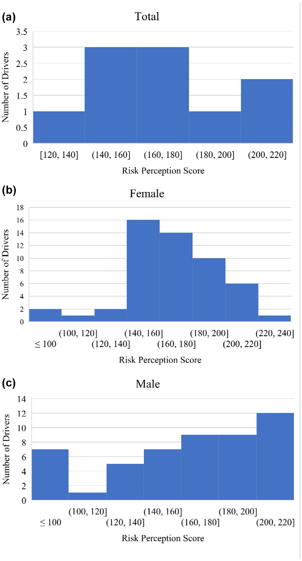
Driver risk perception distribution: (a) total drivers, (b) female drivers, and (c) male drivers.

Table 2.

Summary of Driver Risk Perception and Demographic Information

Age	Female		Male
Age	Sample size	Risk perception*	Sample size	Risk perception*
≤24	32	(120, 198)	20	(112, 192)
25–59	11	(150, 205)	17	(123, 206)
≥60	9	(164, 221)	13	(147, 219)

Note: ^*A higher risk perception score indicates a higher level of caution.

Headway Profile by Driver Types

Figure 3 presents the headway profile by driver types at four WZ configurations. It was stated that young drivers are more aggressive and have higher risks of being involved in fatal crashes when compared with other age groups ( 49 ), which is consistent with the lower risk perception score (more aggressive driver) from young drivers. Interestingly, young drivers maintained a longer time headway than middle-aged drivers. From four WZ configurations in this study, middle-aged drivers typically maintained the shortest time headway among all age groups.

Figure 3.

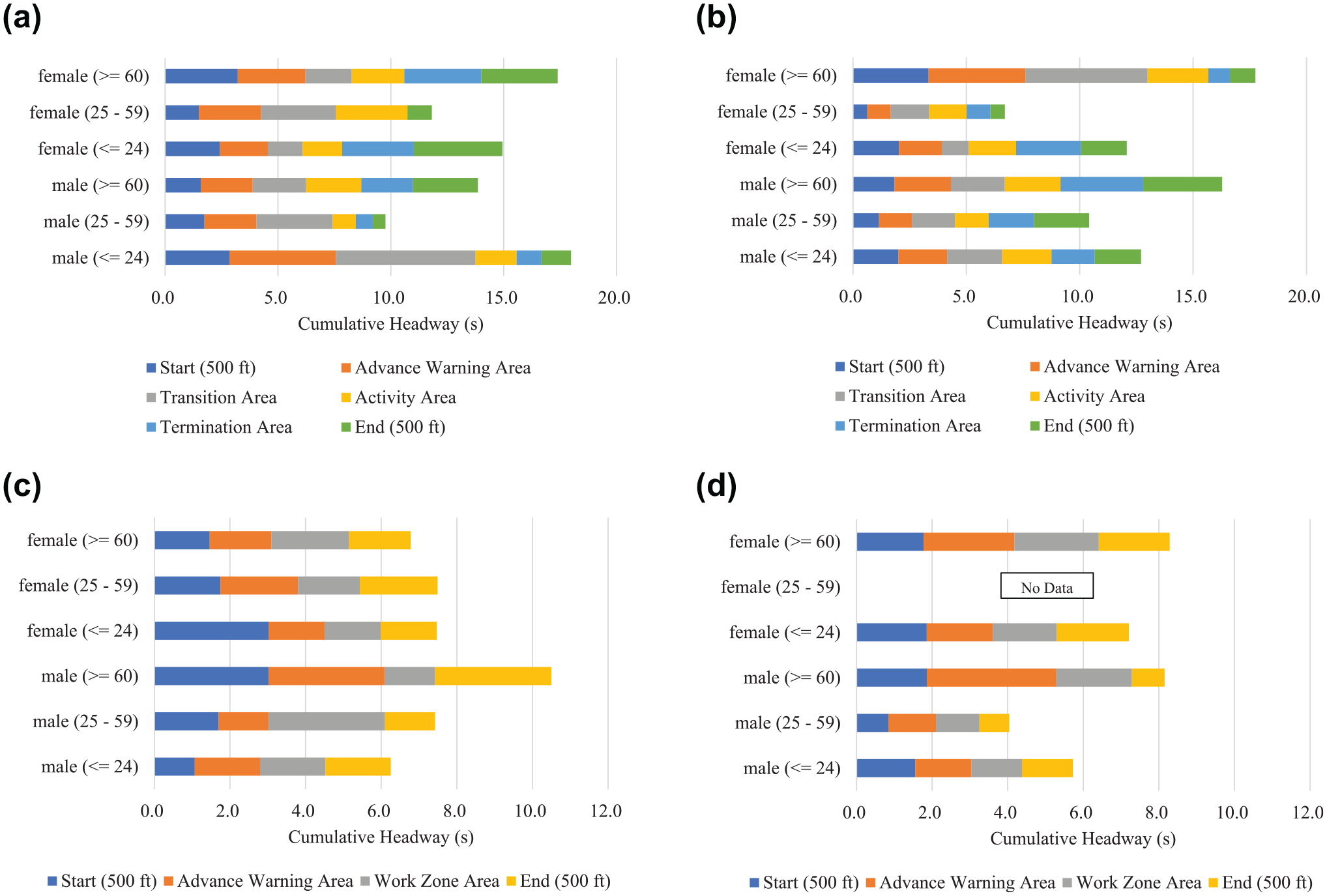
Headway profile by driver types: (a) LC 2-1, (b) LC 3-2, (c) SC 2-2, and (d) SC 3-3.

Headway selection tables before, during, and after WZ by different driver types at four selected WZ configurations (LC 2-1, LC 3-2, SC 2-2, and SC 3-3) were developed. Tables 3 and 4 summarize the details of headway distribution and driver characteristics (gender, age group, and driver risk perceptions). It includes the 95% confidence interval, mean values of risk perception scores, and headways from drivers by age group and gender.

Table 3.

Headway Selection Table by Driver Characteristics: LC 2-1 and LC 3-2

Criteria			LC 2-1			LC 3-2
Start (500 ft)	Gender	Age	Average headway (s)	95% CI of headways (s)	Average risk score	Average headway (s)	95% CI of headways (s)	Average risk score
	Female	Subtotal	2.7	(1.3, 4.2)	176.0	2.3	(1.0, 3.5)	170.5
		≤24	2.4	(2.3, 2.5)	142.0	2.0	(0.9, 3.2)	149.9
		25–59	1.5	(1.2, 1.8)	160.5	0.6	(0.6, 0.6)	196.0
		≥60	3.2	(1.7, 4.7)	185.9	3.3	(2.7, 3.9)	203.0
	Male	Subtotal	1.9	(0.8, 2.9)	191.0	1.8	(1.0, 2.6)	147.8
		≤24	2.8	(2.0, 3.7)	146.0	2.0	(1.3, 2.7)	151.7
		25–59	1.7	(1.0, 2.5)	189.7	1.2	(0.9, 1.4)	164.7
		≥60	1.6	(0.5, 2.6)	207.8	1.8	(1.8, 1.9)	192.0
	Grand total		2.4	(1.0, 3.8)	181.5	1.9	(1.0, 2.9)	153.6
Advance warning area	Gender	Age	Average headway (s)	95% CI of headways (s)	Average risk score	Average headway (s)	95% CI of headways (s)	Average risk score
	Female	Subtotal	2.9	(1.5, 4.2)	174.3	1.8	(0.5, 3.2)	171.9
		≤24	2.1	(1.7, 2.5)	142.0	1.9	(0.6, 3.2)	163.1
		25–59	2.8	(1.7, 2.5)	166.6	1.0	(0.2, 1.8)	196.0
		≥60	3.0	(1.6, 4.4)	181.8	4.3	(3.9, 4.6)	203.0
	Male	Subtotal	2.6	(1.3, 4.2)	185.4	1.9	(1.0, 2.8)	151.9
		≤24	4.7	(3.6, 5.8)	146.0	2.1	(1.3, 3.0)	152.6
		25–59	2.3	(0.7, 3.9)	167.0	1.5	(0.7, 2.2)	165.5
		≥60	2.3	(1.0, 3.6)	207.1	2.5	(1.8, 3.1)	103.5
	Grand total		2.8	(1.3, 4.2)	178.0	1.9	(0.8, 2.9)	157.6
Transition area	Gender	Age	Average headway (s)	95% CI of headways (s)	Average risk score	Average headway (s)	95% CI of headways (s)	Average risk score
	Female	Subtotal	2.4	(1.1, 3.7)	170.5	1.4	(0.3, 2.6)	163.6
		≤24	1.5	(1.5, 1.6)	142.0	1.2	(0.4, 2.0)	156.2
		25–59	3.3	(1.4, 5.2)	165.4	1.7	(1.0, 2.4)	196.0
		≥60	2.0	(1.5, 2.6)	177.0	5.4	(5.4, 5.4)	203.0
	Male	Subtotal	3.1	(0.8, 5.4)	192.2	2.2	(0.2, 4.2)	162.3
		≤24	6.2	(5.9, 6.5)	146.0	2.4	(1.4, 3.5)	147.0
		25–59	3.4	(0.1, 6.8)	173.8	1.9	(0.0, 4.5)	169.5
		≥60	2.4	(1.0, 3.8)	207.5	2.4	(0.9, 3.8)	190.4
	Grand total		2.7	(0.9, 4.4)	178.5	1.9	(0.1, 3.7)	162.8
Activity area	Gender	Age	Average headway (s)	95% CI of headways (s)	Average risk score	Average headway (s)	95% CI of headways (s)	Average risk score
	Female	Subtotal	2.4	(1.0, 3.9)	173.6	2.0	(0.7, 3.4)	169.1
		≤24	1.8	(0.1, 3.4)	141.8	2.1	(0.7, 3.5)	158.1
		25–59	3.2	(0.8, 5.5)	162.8	1.7	(0.7, 2.6)	193.3
		≥60	2.3	(1.4, 3.3)	180.5	2.7	(1.2, 4.2)	203.0
	Male	Subtotal	2.1	(0.6, 3.6)	195.9	1.9	(0.8, 3.0)	154.1
		≤24	1.8	(0.5, 3.2)	146.0	2.2	(1.1, 3.3)	140.1
		25–59	1.0	(0.8, 1.2)	202.0	1.5	(0.5, 2.5)	167.1
		≥60	2.4	(0.9, 4.0)	206.9	2.5	(1.4, 3.5)	155.7
	Grand total		2.3	(0.8, 3.8)	181.4	1.9	(0.7, 3.1)	158.6
Termination area	Gender	Age	Average headway (s)	95% CI of headways (s)	Average risk score	Average headway (s)	95% CI of headways (s)	Average risk score
	Female	Subtotal	3.4	(1.8, 5.0)	177.0	1.6	(0.7, 2.6)	184.2
		≤24	3.2	(2.0, 4.4)	141.2	2.9	(2.4, 3.3)	158.0
		25–59	NA	NA	NA	1.0	(0.5, 1.5)	190.9
		≥60	3.4	(1.8, 5.1)	182.1	1.0	(0.6, 1.3)	203.0
	Male	Subtotal	1.7	(0.2, 3.1)	190.6	2.0	(0.8, 3.2)	140.8
		≤24	1.1	(1.0, 1.2)	146.0	1.9	(0.8, 3.0)	137.6
		25–59	0.8	(0.3, 1.2)	202.0	2.0	(0.6, 3.4)	163.8
		≥60	2.3	(0.5, 4)	203.9	3.6	(3.6, 3.7)	192.0
	Grand total		2.8	(1.1, 4.6)	181.5	1.9	(0.7, 3.1)	159.8
End (500 ft)	Gender	Age	Average headway (s)	95% CI of headways (s)	Average risk score	Average headway (s)	95% CI of headways (s)	Average risk score
	Female	Subtotal	2.9	(1.2, 4.6)	180.9	1.5	(0.9, 2.1)	179.7
		≤24	3.9	(3.9, 4.0)	141.0	2.0	(1.6, 2.5)	154.2
		25–59	1.1	(0.9, 1.2)	171.0	0.6	(0.6, 0.7)	179.0
		≥60	3.4	(1.7, 5.0)	185.6	1.1	(0.8, 1.4)	203.0
	Male	Subtotal	2.1	(0.2, 3.9)	191.2	2.2	(0.9, 3.5)	153.5
		≤24	1.3	(1.3, 1.3)	146.0	2.1	(0.7, 3.4)	146.4
		25–59	0.6	(0.5, 0.6)	202.0	2.4	(1.2, 3.7)	163.9
		≥60	2.9	(0.8, 5.0)	203.5	3.5	(3.4, 3.6)	192.0
	Grand total		2.6	(0.8, 4.4)	184.6	2.0	(0.8, 3.2)	161.9

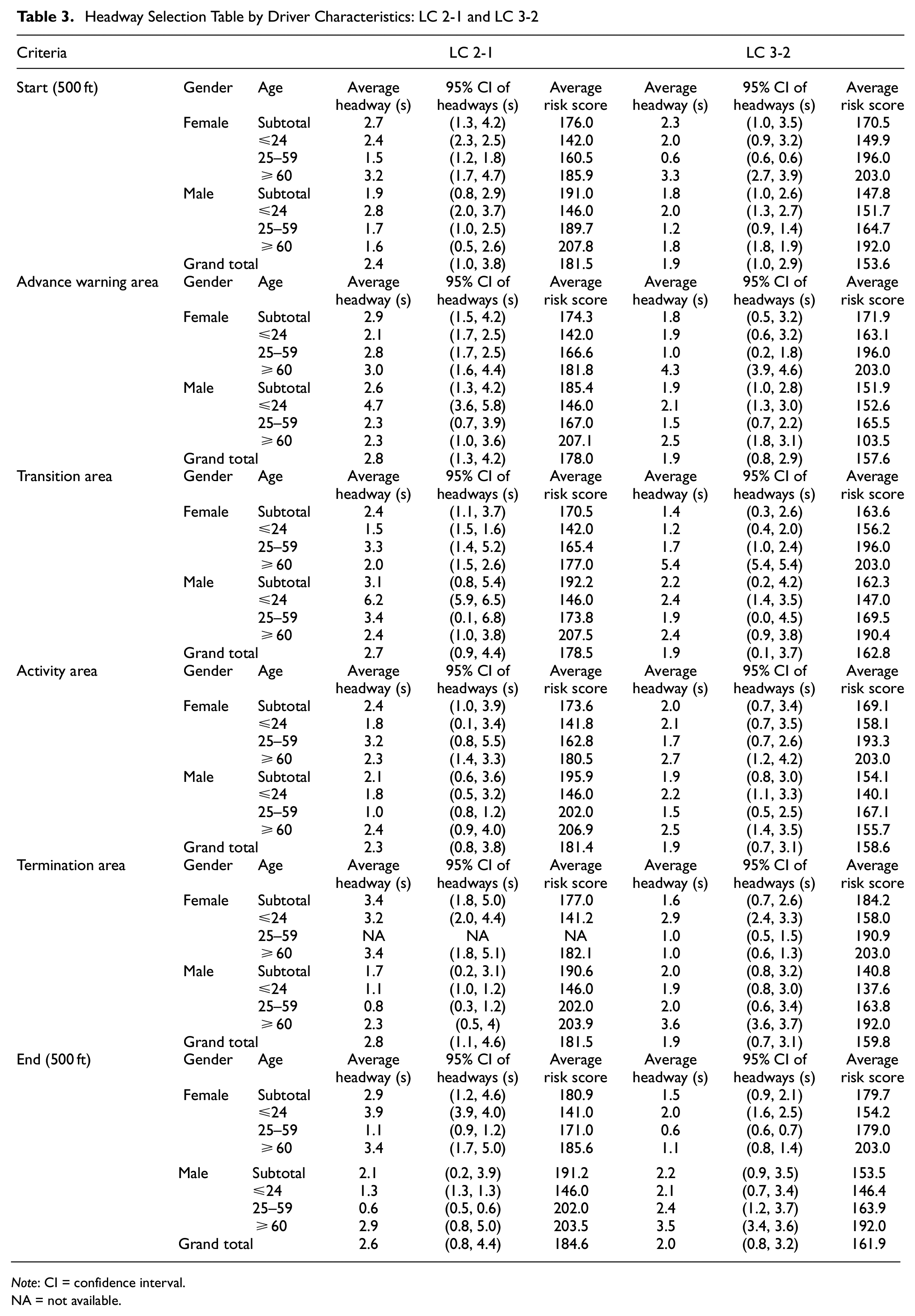
Note: CI = confidence interval.NA = not available.

Table 4.

Headway Selection Table by Driver Characteristics: SC 2-2 and SC 3-3

Criteria			SC 2-2			SC 3-3
Start (500 ft)	Gender	Age	Average headway (s)	95% CI of headways (s)	Average risk score	Average headway (s)	95% CI of headways (s)	Average risk score
	Female	Subtotal	2.1	(0.7, 3.6)	176.7	1.8	(0.9, 2.8)	171.2
		≤24	3.0	(1.2, 4.9)	154.3	1.9	(1.0, 2.8)	168.0
		25–59	1.7	(1.6, 1.9)	192.0	NA	NA	NA
		≥60	1.5	(1.2, 1.7)	192.7	1.8	(0.6, 3.0)	180.9
	Male	Subtotal	2.0	(0.8, 3.1)	184.6	1.5	(0.7, 2.3)	161.8
		≤24	1.1	(1.0, 1.1)	191.0	1.6	(0.7, 2.4)	153.1
		25–59	1.7	(0.4, 3.0)	201.0	0.8	(0.1, 1.6)	165.6
		≥60	3.0	(2.9, 3.2)	156.5	1.9	(1.8, 1.9)	188.6
	Grand total		2.1	(0.7, 3.4)	179.2	1.7	(0.8, 2.6)	167.2
Advance warning area	Gender	Age	Average headway (s)	95% CI of headways (s)	Average risk score	Average headway (s)	95% CI of headways (s)	Average risk score
	Female	Subtotal	1.6	(0.9, 2.3)	180.9	1.9	(0.7, 3.2)	173.8
		≤24	1.5	(0.8, 2.2)	158.5	1.8	(0.6, 2.9)	169.7
		25–59	2.1	(1.2, 2.9)	192.0	NA	NA	NA
		≥60	1.6	(1.0, 2.2)	191.6	2.4	(1.1, 3.7)	184.0
	Male	Subtotal	1.8	(0.5, 3.1)	194.1	1.6	(0.5, 2.8)	166.0
		≤24	1.7	(0.9, 2.6)	187.6	1.5	(0.7, 2.3)	157.8
		25–59	1.3	(0.4, 2.2)	201.0	1.3	(0.1, 2.7)	192.8
		≥60	3.1	(1.4, 4.8)	187.8	3.4	(1.6, 5.3)	193.8
	Grand total		1.7	(0.7, 2.6)	186.1	1.8	(0.6, 3.1)	171.6
Work zone area	Gender	Age	Average headway (s)	95% CI of headways (s)	Average risk score	Average headway (s)	95% CI of headways (s)	Average risk score
	Female	Subtotal	1.6	(0.9, 2.3)	180.9	1.8	(0.6, 3.0)	172.7
		≤24	1.5	(0.8, 2.2)	158.5	1.7	(0.5, 2.9)	167.8
		25–59	1.6	(1.0, 2.2)	191.6	N/A	N/A	N/A
		≥60	2.1	(1.2, 2.9)	192.0	2.2	(1.4, 3.1)	190.9
	Male	Subtotal	1.8	(0.5, 3.1)	194.1	1.4	(0.6, 2.2)	167.7
		≤24	1.7	(0.9, 2.6)	187.6	1.3	(0.6, 2.0)	161.4
		25–59	3.1	(1.4, 4.8)	187.8	1.2	(0.4, 1.9)	170.3
		≥60	1.3	(0.4, 2.2)	201.0	2.0	(1.1, 2.9)	198.0
	Grand total		1.6	(0.6, 2.6)	186.6	1.7	(0.6, 2.7)	171.1
End (500 ft)	Gender	Age	Average headway (s)	95% CI of headways (s)	Average risk score	Average headway (s)	95% CI of headways (s)	Average risk score
	Female	Subtotal	1.6	(0.9, 2.3)	180.9	1.9	(1.0, 2.8)	175.0
		≤24	1.5	(0.8, 2.2)	158.5	1.9	(1.0, 2.8)	172.7
		25–59	2.1	(1.2, 2.9)	192.0	N/A	N/A	N/A
		≥60	1.6	(1.0, 2.2)	191.6	1.9	(0.7, 3.1)	198.0
	Male	Subtotal	1.8	(0.5, 3.1)	194.1	1.1	(0.4, 1.8)	172.8
		≤24	1.7	(0.9, 2.6)	187.6	1.3	(0.9, 1.8)	168.3
		25–59	1.3	(0.4, 2.2)	201.0	0.8	(0.6, 0.9)	171.0
		≥60	3.1	(1.4, 4.8)	187.8	0.9	(0.1, 1.9)	181.5
	Grand total		1.7	(0.7, 2.8)	182.8	1.6	(0.7, 2.6)	174.3

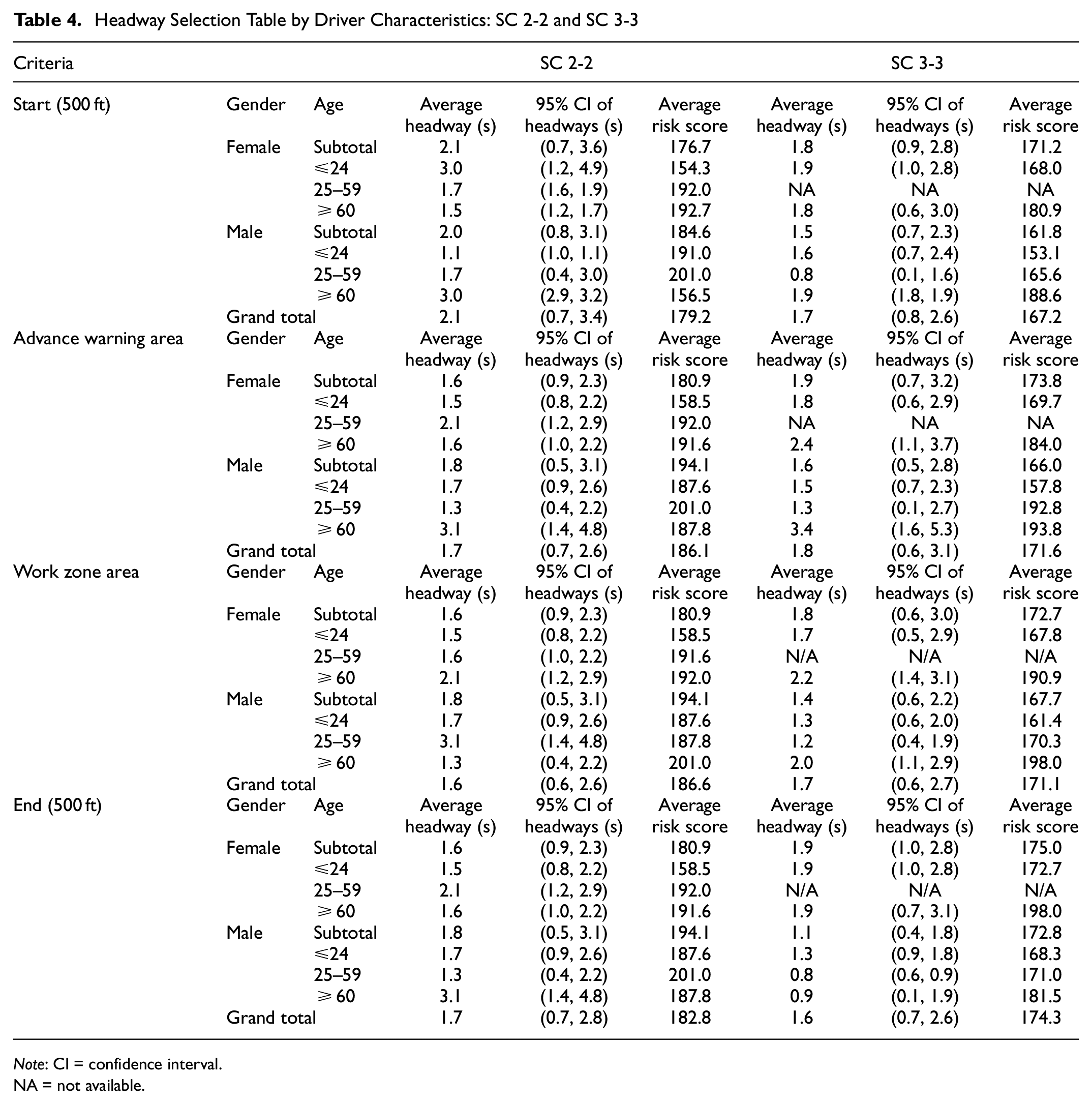
Note: CI = confidence interval.NA = not available.

The headway distributions from different drivers traversing various WZ can be useful for the purpose of estimating and calibrating WZ capacity models. The desired time headway parameter (CC1) in VISSIM is static through all WZ consecutive sections, although it was suggested that desired time headway should be modeled as a distribution rather than a static value when data are available ( 50 ). Thus, if headway distribution models built for different driver characteristics are used in lieu of a static value in VISSIM, a more accurate capacity estimation can be captured.

Headway Comparison

The headway distributions by different WZ consecutive sections are illustrated in Figure 4. Boxplots were utilized to detect potential outliers, which were filtered if they were beyond the upper limit or lower limit. It can be found that vehicles maintain different headways either in different WZ sections or configurations. For instance, at WZ configuration LC 2-1 as presented in Figure 4a, the mean headways from start section to end section (Table 3) are 2.4, 2.8, 2.7, 2.3, 2.8, and 2.6 s, respectively. From the boxplots, the range of the upper quartile (75%) and lower quartile (25%) in mean headway have the tendency to decrease as vehicles move from start section to transition area. The mean headway began to increase after traversing the activity area. While for LC 3-2, the mean headway throughout the entire WZ remained unchanged at 1.9 s (Table 3). As for shoulder closure, the mean headways from the start to the end at SC 2-2 are 2.1, 1.8, 1.6, and 1.8 s (Table 4). At SC 3-3, headways were stable with minor changes ranging from 1.6 to 1.8 s traversing WZs (Table 4). This might be indicating that with more through lanes, WZ activity will have less impact on drivers.

Figure 4.

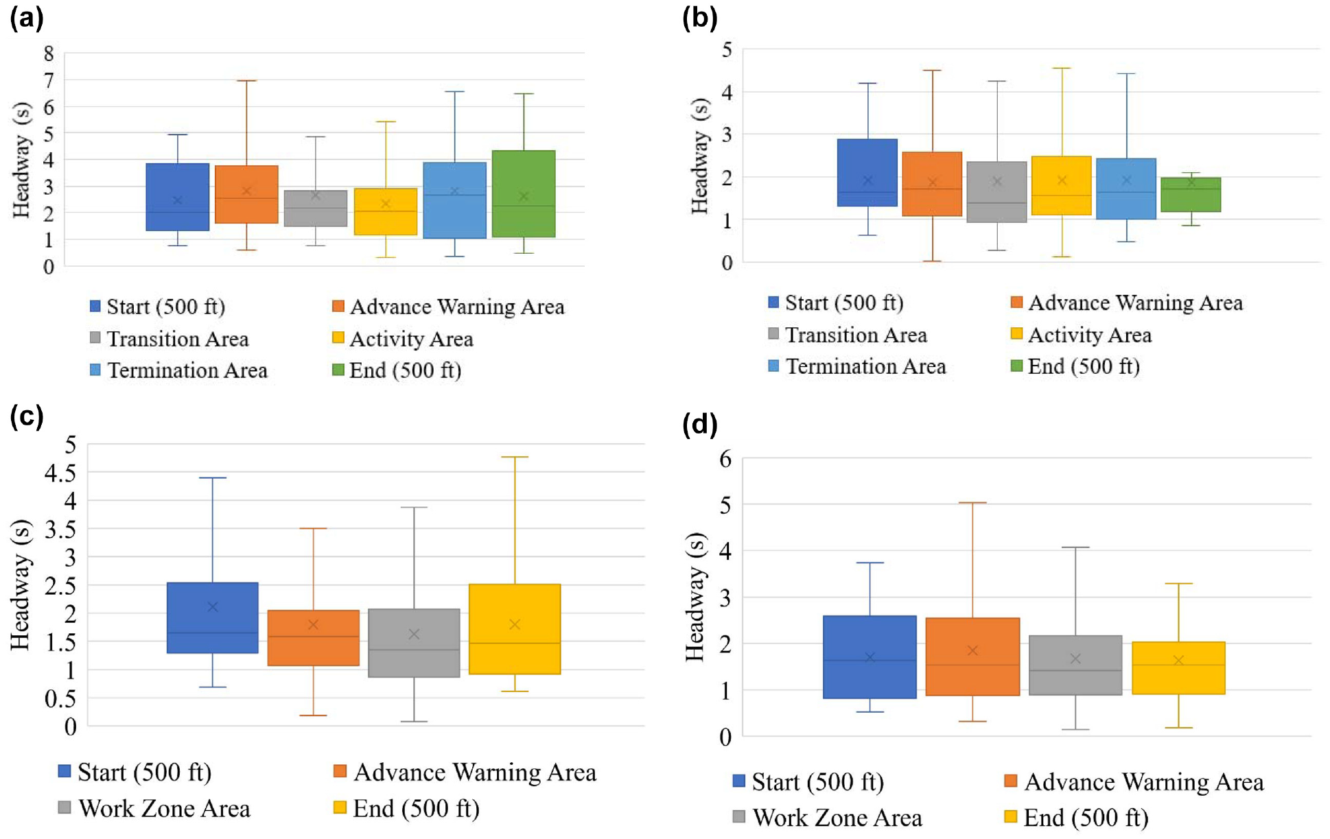
Headway distribution by work zone areas: (a) LC 2-1, (b) LC 3-2, (c) SC 2-2, and (d) SC 3-3.

As shown in Figure 5, GAM estimated the best-fitted curves of time headway throughout WZ at four WZ configurations. Figure 5a presents the time headway estimation for LC 2-1. The time headway tends to increase when drivers approach the advance warning area. It starts to decrease when drivers are in the advance warning area. The decreasing trend continues until drivers are at the end of the activity area. The smallest time headway occurs in the activity area. The time headway quickly increases after drivers enter the termination area. For LC 3-2 (Figure 5b), fluctuations are expected before the activity area. The time headway tends to decrease consistently when drivers approach the activity area. The smallest headway was estimated in the activity area. The time headway started to increase in the termination area where the barrier drums are removed.

Figure 5.

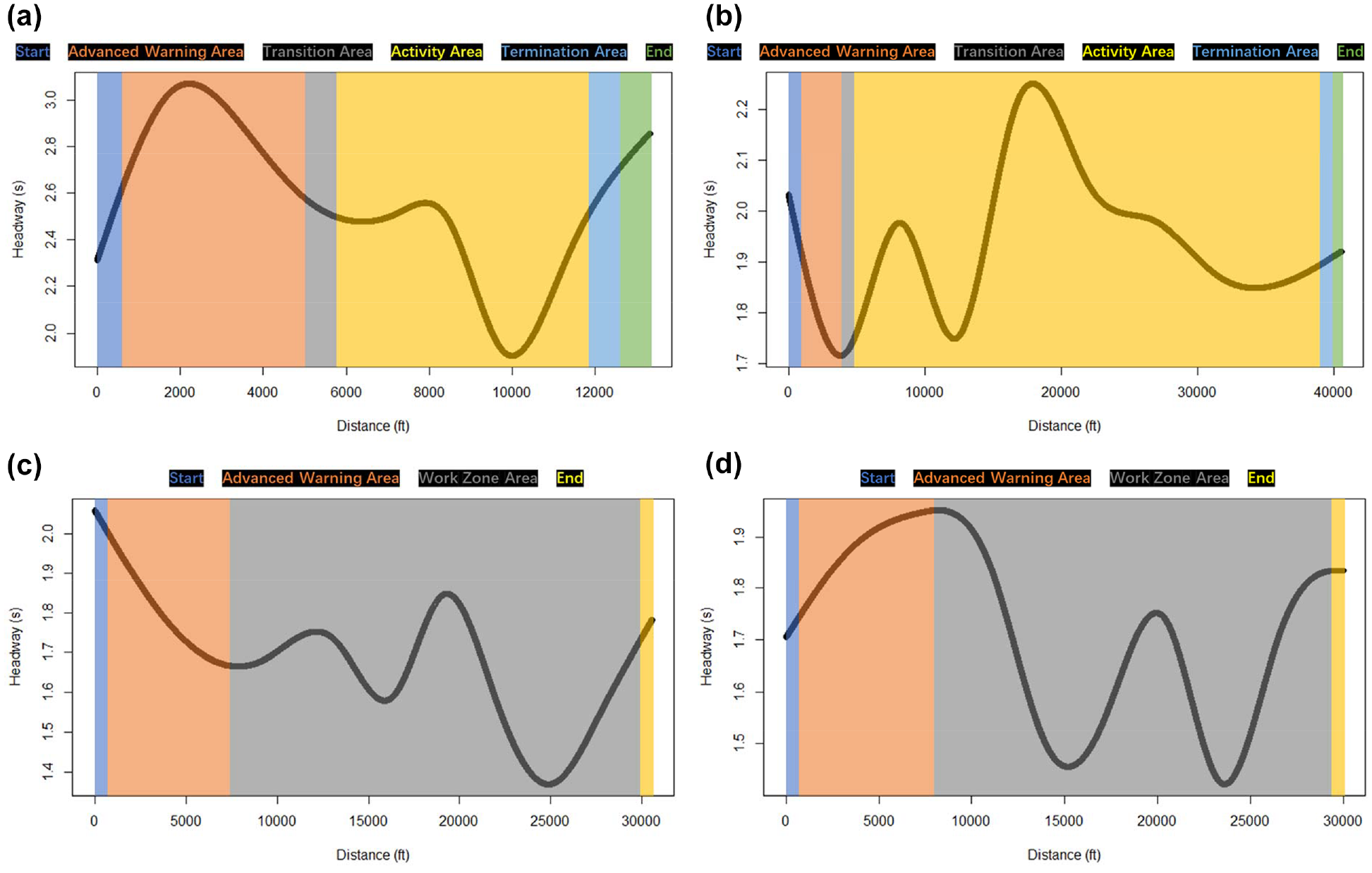
Headway estimation by work zone sections: (a) LC 2-1, (b) LC 3-2, (c) SC 2-2, and (d) SC 3-3.

Figure 5c presents the estimated headway for SC 2-2. The overall trend illustrates that time headway decreases until drivers start to leave the WZ. For SC 3-3 (Figure 5d), the two smallest headway points were observed. The first one occurs where the shoulder has been fully closed with limited shoulder clearance. The second one can be found where drivers approach the activity area. A decreasing trend in time headway can be noticed before these two points and an increasing trend shows up afterward.

Speed Analysis

Speed Profile

Speed profiles by GAM are presented in Figure 6, which shows speed distributions in the entire WZ at four configurations. The x-axis is the length (feet) and the y-axis is the speed (mph). The black dots are the speed data from SHRP 2 NDS time-series reports, one trace coming from one traversal. The red lines are the best-fitted curves by using GAM. After reviewing the forward-view videos, it was found that the reduced speed limit sign (55 mph) only appeared at LC 2-1 configuration. From Figure 6a, it is observed that at LC 2-1 WZ, speeds decreased when approaching WZ, but drivers were only compliant with 55 mph speed limit during the transition area. Their speeds increased when entering the activity area. At SC 2-2 WZ, there is a speed reduction between 10,000 and 20,000 ft, in response to the presence of concrete barriers instead of drums. The other two configurations did not observe significant speed changes during the entire WZ traversal.

Figure 6.

Speed distribution by work zone sections: (a) LC 2-1, (b) LC 3-2, (c) SC 2-2, and (d) SC 3-3.

Speed Change Point

Speed change point detection was used to identify points where both mean and variance of speeds had significant changes. Figure 7 presents speed change points at four WZ configurations. The x-axis is the data point index and the y-axis is the speed (mph). The red arrow indicates the location of a speed change point in WZs. As aforementioned, only LC 2-1 presented the speed reduction requirement from the reduced speed limit sign. It can be seen in Figure 7a that the mean speed began to decrease by 8 mph after entering the advance warning area and increased back to initial speeds after drivers saw the end of the WZ drums. At LC 3-2 (Figure 7b), a slight speed increase was observed (2 mph on average) after entering the activity area. This might be because the traffic volume was much lower than the capacity, so the WZ had less impact on drivers. The mean speed then decreased by 4 mph when drivers were near the activity area. For SC 2-2 (Figure 7c), the mean speed was significantly reduced by 5 mph where concrete barriers showed narrowed shoulder clearance. It increased by 2 mph near the end of the WZ area. Slight speed decreases (2–3 mph) at SC 3-3 (Figure 7d) were observed, which was likely led by the downstream merging behavior from freeway on-ramps.

Figure 7.

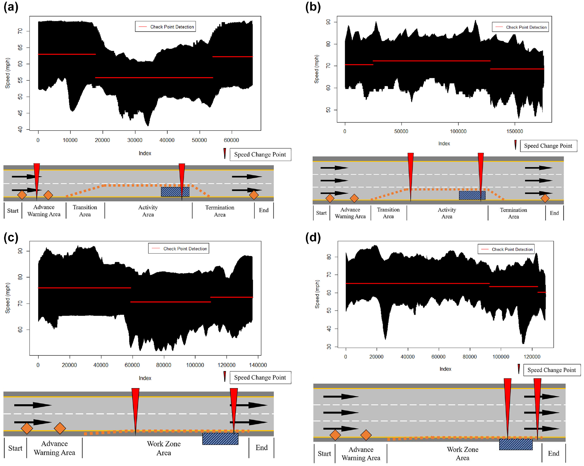
Speed change point detection: (a) LC 2-1, (b) LC 3-2, (c) SC 2-2, and (d) SC 3-3.

The speed profile can be used to improve or calibrate planning and simulation tools. For instance, the free-flow speed, average speed, minimum speed, distance traveled during speed change cycle, average speed in queue, and so forth from QUEWZ, which were based on outdated field data and methodology ( 13 ), can be modified from WZ NDS trip data. The speed change point detection can be used to assist with the WZ setup process. It can help transportation agencies better understand driver behavior in WZs.

Relationship between Speed and Headway

Most evidence of the relationship between speed and headway seems vague because the capacity was much more than the traffic volumes per data. However, 10 breakdown cases in SC 3-3 showed the potential for modeling the relationship between speed and time headway. The speed and time headway follows the reciprocal function, which indicates a linear correlation can be found between speed and 1/headway (Figure 8). With an R-squared of 0.79, the correlation can be written as:

\begin{matrix} \frac{1}{T i m e H e a d w a y (s)} = 0.01779 \times S p e e d (m p h) \end{matrix}

(3)

Figure 8.

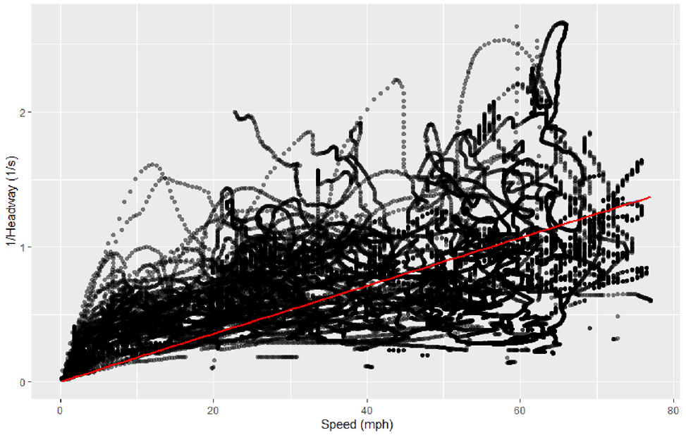
Fitted model between speed and time headway.

Thus, the estimated relationship between speed and time headway can be seen in Figure 9. When a breakdown occurs, time headway will decrease with a shrinking decrease rate. The space headway can be calculated as:

\begin{matrix} \begin{matrix} Space Headway (ft) = Time Headway (s) \times Speed (ft / s) \\ = Time Headway (s) \times [Speed (mph) \times 1.47] (ft / s) \\ = \frac{1}{0.01779} \times 1.47 \approx 82 ft \end{matrix} \end{matrix}

(4)

Figure 9.

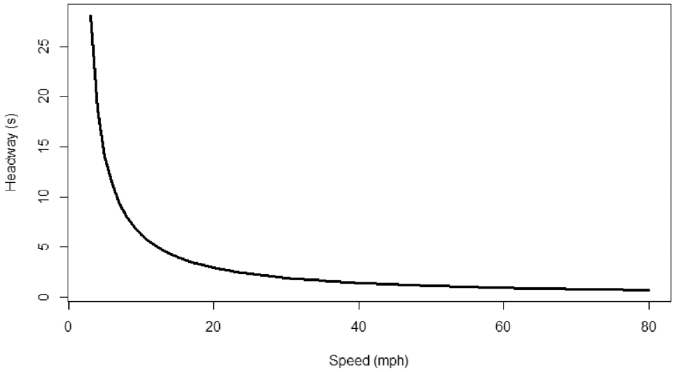
Relationship between speed and time headway.

Thus, the average space headway for an individual vehicle under WZ breakdown condition (SC 3-3) is roughly 82 ft.

Conclusion

This study utilized SHRP 2 NDS data to develop headway selection tables based on driver characteristics and to establish speed profiles in four freeway WZ configurations. Key findings are summarized as follows:

Headway selection tables revealed that car-following behaviors are highly variable, differing according to driver’s gender, age group, and risk perceptions, which influences WZ capacity. Furthermore, headways are different at consecutive WZ sections; selecting appropriate headway would be helpful when predicting WZ capacity from simulation models. These findings suggest that WZ capacity may be modeled more accurately if separate headway distributions are constructed for different driver characteristics. Such headway selection is essential to replicate the real-world variability and ultimately to capture more accurate estimates of capacity.

Speed profiles from four WZ configurations indicated that shoulder closure typically does not have a significant impact on speeds under non-breakdown conditions. For lane closure conditions, speeds decrease when drivers approach the transition area and increase when they are near the termination area. The mean speed reduction at LC 2-1 was 8 mph from 63 mph to 55 mph (reduced speed limit) when entering the advance warning area and the speed increased back to initial speeds after the activity area. At LC 3-2, the mean speed reduction of 4 mph from 72 mph to 68 mph was observed when drivers were approaching the activity area. For SC 2-2, the mean speed was reduced by 5 mph from 76 mph to 71 mph where concrete barriers appeared with narrowed shoulder clearance. There was no significant speed change at SC 3-3.

The relationship between speed and time headway was modeled based on 10 breakdown events at SC 3-3 condition. A linear correlation was found between speed and 1/headway with an R-squared of 0.79. Similar models can be developed for the other WZ configurations with more data.

Limitations

This is the first study that applied SHRP 2 NDS data to study the effect of driver characteristics on headway selection and speed distribution over the entire WZ areas. The current SHRP 2 NDS database contains limited trips and WZ configurations. It is suggested to collect more NDS data to further validate the headway selection and speed distribution by different driver types in more WZ configurations.

Footnotes

Acknowledgements

The authors would like to thank VTTI for helping with the data request.

Author Contributions

The authors confirm contribution to the paper as follows: study conception and design: D. Xu and H. Zhou; data collection: C. Xu and H. Zhou; analysis and interpretation of results: D. Xu, C. Xue, and H. Zhou; draft manuscript preparation: D. Xu, C. Xue, and H. Zhou. All authors reviewed the results and approved the final version of the manuscript.

Declaration of Conflicting Interests

The author(s) declared no potential conflicts of interest with respect to the research, authorship, and/or publication of this article.

Funding

The author(s) disclosed receipt of the following financial support for the research, authorship, and/or publication of this article: This project was funded by the Region 4 University Research Center led by the University of Florida (Project Number I3).

References

Work Zone Management Program. FHWA Work Zone Facts and Statistics. Federal Highway Administration, U.S. Department of Transportation, Washington, D.C.https://ops.fhwa.dot.gov/wz/resources/facts_stats.htm. Accessed July 5, 2020.

Yeom

Rouphail

N. M.

Rasdorf

Simulation Guidance for Freeway Lane Closure Capacity Calibration. Transportation Research Record: Journal of the Transportation Research Board, 2015. 2553: 82–89.

Weng

Meng

Incorporating Work Zone Configuration Factors into Speed-Flow and Capacity Models. Journal of Advanced Transportation, Vol. 49, No. 3, 2015, pp. 371–384.

Weng

Meng

Decision Tree-Based Model for Estimation of Work Zone Capacity. Transportation Research Record: Journal of the Transportation Research Board, 2011. 2257: 40–50.

Highway Capacity Manual, 6th Edition: A Guide for Multimodal Mobility Analysis . Transportation Research Board, Washington, D.C., 2016.

Weng

Meng

Ensemble Tree Approach to Estimating Work Zone Capacity. Transportation Research Record: Journal of the Transportation Research Board, 2012. 2286: 56–67.

Heaslip

Kondyli

Arguea

Elefteriadou

Sullivan

Estimation of Freeway Work Zone Capacity through Simulation and Field Data. Transportation Research Record: Journal of the Transportation Research Board, 2009. 2130: 16–24.

Kan

Ramezani

Benekohal

R. F.

Calibration of VISSIM for Freeway Work Zones with Time Varying Capacity. Presented at 93rd Annual Meeting of the Transportation Research Board, Washington, D.C., 2014.

Chatterjee

Edara

Menneni

Sun

Replication of Work Zone Capacity Values in a Simulation Model. Transportation Research Record: Journal of the Transportation Research Board, 2009. 2130: 138–148.

10.

Heaslip

Jain

Elefteriadou

Estimation of Arterial Work Zone Capacity Using Simulation. Transportation Letters, Vol. 3, No. 2, 2011, pp. 123–134.

11.

Benekohal

R. F.

Kaja-Mohideen

A. Z.

Chitturi

M. V.

Evaluation of Construction Work Zone Operational Issues: Capacity, Queue, and Delay. Publication ITRC FR 00/01-4. Illinois Transportation Research Center, Urbana-Champaign, 2003.

12.

Ramezani

Benekohal

R. F.

Work Zones as a Series of Bottlenecks. Transportation Research Record: Journal of the Transportation Research Board, 2012. 2272: 67–77.

13.

Ishimaru

Hallenbeck

QUEWZ Work Zone Software: Literature Search and Methodology Review. WA-RD 888.1. Washington State Department of Transportation, Olympia, 2019.

14.

Trask

Aghdashi

Schroeder

Rouphail

FREEVAL-WZ Users Guide. North Carolina State University, Raleigh, 2015.

15.

Van Schagen

Welsh

Backer-Grondahl

Hoedemaeker

Lotan

Morris

Sagberg

Winkelbauer

Towards a Large-Scale European Naturalistic Driving Study: A Final Report of PROLOGUE. SWOV Institute for Road Safety Research, Leidschendam, Netherlands, 2011.

16.

Dingus

T. A.

Hankey

J. M.

Antin

J. F.

Lee

S. E.

Eichelberger

Stulce

K. E.

McGraw

Perez

Stowe

Naturalistic Driving Study: Technical Coordination and Quality Control. SHRP 2 Report S2-S06-RW-1. FHWA, U.S. Department of Transportation, Washington, D.C., 2015.

17.

Zhou

H. H.

Turochy

Evaluation of Work Zone Mobility by Utilizing Naturalistic Driving Study Data. Southeastern Transportation Research, Innovation, Development and Education Center, University of Florida, Gainesville, 2019.

18.

May

A. D.

Traffic Flow Fundamentals. Prentice Hall Inc., Englewood Cliffs, NJ, 1990.

19.

Zhang

Vehicle Type-Specific Headway Analysis Using Freeway Traffic Data. Transportation Research Record: Journal of the Transportation Research Board, 2009. 2124: 222–230.

20.

Cowan

R. J.

Useful Headway Models. Transportation Research, Vol. 9, No. 6, 1975, pp. 371–375.

21.

Sun

Benekohal

R. F.

Analysis of Work Zone Gaps and Rear-End Collision Probability. Journal of Transportation and Statistics, Vol. 8, No. 2, 2006, pp. 71–86.

22.

Greenberg

The Log-Normal Distribution of Headways. Australian Road Research, Vol. 2, No. 7, 1966, pp. 14–18.

23.

Hoogendoorn

S. P.

Bovy

P. H. L.

A New Estimation Technique for Vehicle-Type Specific Headway Distributions. Transportation Research Record: Journal of the Transportation Research Board, 1998. 1646: 18–28.

24.

Weng

Meng

Fwa

T. F.

Vehicle Headway Distribution in Work Zones. Transportmetrica A: Transport Science, Vol. 10, No. 4, 2014, pp. 285–303.

25.

Migletz

Graham

Hess

Anderson

Harwood

Bauer

Effectiveness and Implementability of Procedures for Setting Work Zone Speed Limits. Publication NCHRP Project 3-41(2). Graham-Migletz Enterprises, Independence, MO, 1998.

26.

Bham

G. H.

Mohammadi

M. A.

Evaluation of Work Zone Speed Limits: An Objective and Subjective Analysis of Work Zones in Missouri. No. MATC REPORT 25-1121-0001-119. Mid-America Transportation Center, Lincoln, NE, 2011.

27.

Benekohal

R. F.

Mohideen

A. Z. K.

Chitturi

M. V.

Methodology for Estimating Operating Speed and Capacity in Work Zones. Transportation Research Record: Journal of the Transportation Research Board, 2004. 1883: 103–111.

28.

Xue

Zhou

Impacts of Directional Rumble Strips on Vehicle Speeds and Driver Behavior at Freeway Off-Ramps. Journal of Transportation Engineering, Part A: Systems, Vol. 146, No. 9, 2020, p. 04020093.

29.

Migletz

Graham

J. L.

Anderson

I. B.

Harwood

D. W.

Bauer

K. M.

Work Zone Speed Limit Procedure. Transportation Research Record: Journal of the Transportation Research Board, 1999. 1657: 24–30.

30.

Pesti

McCoy

P. T.

Long-Term Effectiveness of Speed Monitoring Displays in Work Zones on Rural Interstate Highways. Transportation Research Record: Journal of the Transportation Research Board, 2001. 1754: 21–30.

31.

Bai

Comparison of Characteristics between Fatal and Injury Accidents in the Highway Construction Zones. Journal of Safety Science, Vol. 46, 2008, pp. 646–660.

32.

Campbell

K. L.

The SHRP 2 Naturalistic Driving Study: Addressing Driver Performance and Behavior in Traffic Safety. TR News, No. 282, September–October 2012, pp. 30–35.

33.

Victor

Dozza

Bärgman

Boda

C. N.

Engström

Flannagan

Lee

J. D.

Markkula

Analysis of Naturalistic Driving Study Data: Safer Glances, Driver Inattention, and Crash Risk. No. SHRP 2 Report S2-S08A-RW-1. National Academies of Sciences, Engineering, and Medicine, Washington, D.C., 2015.

34.

Foss

R. D.

Goodwin

A. H.

Distracted Driver Behaviors and Distracting Conditions among Adolescent Drivers: Findings from a Naturalistic Driving Study. Journal of Adolescent Health, Vol. 54, No. 5, 2014, pp. S50–S60.

35.

Zhou

Xue

Transportation Research Circular E-C243: Interchange Deceleration Lane Design Based on Naturalistic Driving Speeds and Deceleration Rates. TRB, National Research Council, Washington, D.C., 2019.

36.

Hallmark

Smadi

Sharma

Evaluation of Work Zone Safety Using the SHRP 2 Naturalistic Driving Study Data. Center for Transportation Research and Education, Iowa State University’s Institute for Transportation, Ames. http://shrp2.transportation.org/Documents/03-SHRP2%20IAP%20Round%204-MNWork%20Zones.pdf. Accessed July 5, 2020.

37.

Edara

Smardi

A Multidisciplinary Approach to Investigate Work Zone Safety Using SHRP 2 Safety Data. University of Missouri, Columbia. https://mtc.intrans.iastate.edu/research/in-progress/a-multidisciplinary-approach-to-investigate-work-zone-safety-using-shrp-2-safety-data/. Accessed July 5, 2020.

38.

Selpi

Kovaceva

Thomson

Analysis of SHRP2 Data to Understand Normal and Abnormal Driving Behavior in Work Zones: Phase II. University of Michigan Transportation Research Institute, Ann Arbor. https://www.chalmers.se/en/projects/Pages/Analysis-of-SHRP2-Data-to-Understand-Normal-and-Abnormal-Driving.aspx. Accessed July 5, 2020.

39.

Transportation Research Board of the National Academies of Science. The 2nd Strategic Highway Research Program Naturalistic Driving Study Dataset. SHRP2 NDS InSight Data Dissemination. https://insight.shrp2nds.us. Accessed July 5, 2020.

40.

Work Zone Management Program. FHWA Road Closure and Lane Closure. Federal Highway Administration, U.S. Department of Transportation, Washington, D.C.https://ops.fhwa.dot.gov/wz/construction/full_rd_closures.htm#lc. Accessed January 5, 2021.

41.

FHWA. The Interstate System: Size of the Job. Highway History, Federal Highway Administration, U.S. Department of Transportation, Washington, D.C.https://www.fhwa.dot.gov/infrastructure/50size.cfm#:∼:text=More%20than%2080%20percent%20of,have%206%20lanes%20or%20more. Accessed January 5, 2021.

42.

FHWA. MUTCD, 2009 Edition. https://mutcd.fhwa.dot.gov/pdfs/2009/pdf_index.htm. Accessed June 19, 2021.

43.

Mathew

T. V.

Rao

K. K.

Introduction to Transportation Engineering. Civil Engineering–Transportation Engineering, NPTEL, IIT Bombay. http://www.cdeep.iitb.ac.in/nptel/Civil% 20Engineering. Accessed July 5, 2020.

44.

Larsen

GAM: The Predictive Modeling Silver Bullet. MultiThreaded. https://multithreaded.stitchfix.com/blog/2015/07/30/gam/. Accessed January 5, 2021.

45.

Hastie

T. J.

Tibshirani

R. J.

Generalized Additive Models, Vol. 43. CRC Press, Boca Raton, FL, 1990.

46.

Wood

S. N.

Generalized Additive Models: An Introduction with R. CRC Press, Boca Raton, FL, 2017.

47.

Wood

M. S.

Package ‘mgcv’, R Package Version 1.29. R Cran, Vienna, Austria, 2015.

48.

Killick

Eckley

Changepoint: An R Package for Changepoint Analysis. Journal of Statistical Software, Vol. 58, No. 3, 2014, pp. 1–19.

49.

Lambert-Bélanger

Dubois

Weaver

Mullen

Bedard

Aggressive Driving Behaviour in Young Drivers (Aged 16 through 25) Involved in Fatal Crashes. Journal of Safety Research, Vol. 43, No. 5–6, 2012, pp. 333–338.

50.

Dong

Houchin

Shafieirad

Hawkins

Knicherbocker

VISSIM Calibration for Urban Freeways. Publication InTrans Project 14-487. Center for Transportation Research and Education, Institute for Transportation, Ames, IA, 2015.