Imputing Parking Usage on Sparsely Monitored Areas Within Amsterdam Through the Application of Machine Learning

Overall Field

An academic survey on smart parking solutions was conducted by Lin et al. over the past 15 years and looked at over 100 papers ( 3 ). A categorisation framework was proposed for the different types of research conducted within the domain of smart parking solutions. This framework offered clarity into the current research, but it demonstrated, in its omission of the topic, the lack of research conducted on the imputation of parking usage in sparsely monitored areas through predictive machine learning methods.

The work by Lin et al. provided guidance on relevant papers based on the types of data sources they used, the two notable ones being non-stationary sensors and crowd sourcing ( 3 ). Papers that looked at non-stationary sensors used cars equipped with LIDAR, Magnetron, and cameras to provide a variety of smart parking solutions and were mainly concerned with the problem of detecting parking occupancy; while none were related to predicting occupancy, they did offer insight into the methodologies used to detect occupancy. The papers that looked at using crowd-sourcing methods to determine parking usage primarily investigated the simulated situation if many individuals volunteered their parking behavior through a mobile application. These papers overlap somewhat with this paper but differ in that they assume complete city scan coverage within ±25 min—which is not the case in the Amsterdam context ( 4 , 7 ).

Predicting Parking for Unseen Areas

Three papers were identified that directly or very closely dealt with the topic of predicting parking usage within sparsely monitored areas, a majority of which comes from Fabian Bock who has been focusing on the topic of unknown parking behavior since 2016.

The work by Bock et al. looked at the performance of random forests (RFs) to predict future parking usage using data that was simulated to resemble mobile app crowd-sourcing and probe vehicle parking detection (analogous to the scanner cars used in Amsterdam) ( 4 ). The research used the San Francisco fixed point parking data to simulate the two cases to predict into a 30 min time horizon ( 8 ). This research assumed that there were sufficient probe vehicles (300 cars) in the city to allow for a 25 min time window for a complete view of the city. This research lends credence to the idea that sensor data in the form of scanner cars can be used to predict for parking behavior if there are enough mobile sensors.

The work by Bock and Sester investigated the performance of using IDW to impute parking usage in adjacent roads from nearby road segments that had continuous sensor data ( 6 ). They found strong correlations between the adjacent parking usage the observed road segment of up to 50 m. They found that IDW was 5% better than taking the aggregated occupation values for the road segments. This research showed that there is a possibility for information gain when considering spatial relations between observations.

The paper by Ionita et al. used Gaussian clustering on the average amenity duration visits to identify pairs of areas that had monitored and unmonitored parking spaces ( 5 ). The paper showed that it is possible to train a model on one area of a city and then use that trained model to predict for another part of the city (that was completely unmonitored) on the condition that they belonged to the same cluster class. This paper also experimented with several machine learning models and determined that gradient boosting methods performed the best. This paper relied on data from San Francisco OpenParking data for the occupancy values.

Auxiliary research of interest includes the work by Bock et al. and Richter et al. ( 9 , 10 ). Bock et al. looked at using clustering to aggregate parking meters according to temporal behavior to simplify the analysis of those devices ( 9 ). The research found that there were distinct parking ticket purchasing behaviors within the city of Hannover, Germany, over a one year time period. Hierarchical clustering was used on the hourly aggregated occupancies of the sold passes. This work is of interest because it can help guide the understanding of different neighborhoods when building predictive models to impute the parking usage, and it lends itself well to the work that was done by Ionita et al. ( 5 ).

Richter et al. investigated how best to forecast parking occupancy with the limited resources available to on-board car navigation systems ( 10 ). They built time-series models that only used parking occupancy figures, and they employed spatial and temporal clustering through the use of complete linkage and dynamic time warping (DTW).

Mobile Parking Sensor Data

The mobile sensor data was obtained internally from the Amsterdam city government. This data provided the sparse observations of parking usage throughout the city and was used to determine the parking pressure for each neighborhood for sparse intervals in time.

Business Rules and Bias

The operation of the scanning devices is outsourced to a third-party private company that is contractually committed to satisfy two performance indicators: (1) the revenue generated from identifying non-valid parking, and (2) the chance that a vehicle without a valid parking right will be detected per hour. A softer rule expects each area to be visited at least once every day.

These business rules result in the mobile scanning devices scanning neighborhoods a certain minimum number of times to meet the performance indicators, but these rules also do not stop them from prioritizing other areas of the city to generate as much revenue as possible. Notably, the centre of Amsterdam is heavily scanned compared with the peripheries of the city. It should be noted that the north of Amsterdam (across the IJ river) was only added to the routes of the mobile scanners at the end of 2018 and thus are under-represented.

These business rules also result in a bias of when a neighborhood is scanned because it will prioritize times when the neighborhoods are likely to have high offender rates. Investigation of the data revealed distinct scanning bias patterns throughout the day: uniform, early morning and/or afternoon, and increasing/decreasing visitation trends as the hours progress.

Large parts of the city are also not scanned during weekends because they become free parking during those periods and thus there is no need for the third-party company to scan those areas. A consequence of this is that the data available for weekends is biased toward neighborhoods that are still scanned. The weekends were thus removed for the cases when models were built on the city and cluster training levels.

The low number of scanning devices results in a spatio-temporal sparse view of the city. Figure 1 is a snapshot example of single mobile probe’s patrol behavior for a day and, by extension, illustrates how a sparse view of the city is obtained when a low number of mobile probes are used.

OPEN IN VIEWER

Figure 1.

Parking locations scanned by a single mobile sensor for the day of September 24, 2017.

Parking Pass Purchases Data

Parking pass purchases were internally obtained from the Nationaal Parkeer Register (NPR) through relations provided by the Amsterdam City Government. The data is a transnational log of various types of parking passes purchases from January 2016 to December 2018.

The NPR data indicated if parking passes were of type: BEWONERP, BEDRIJFP, STADSBREED, or BETAALDP. The data did not provide information on how the first three (long-term) passes were used throughout the city, while the the BETAALDP are for short-term stays and thus offer a good estimate of where and how they are being used. The BETAALDP passes account for ±15% of daily parking usage.

The BETAALDP passes were aggregated for hourly intervals per neighborhood to align with the data generated from the scan data. The aggregation of the BETAALDP parking passes were performed by spatially joining the parking pass purchase locations to the neighborhood geometries and then aggregating statistics about the parking pass purchases on hourly intervals. Four types of aggregations were built: (1) number of passes bought; (2) parking occupation as a function of how much parking time was bought in that hour (i.e., a pass bought at 13:30 will count for 0.5 of a pass at hour 13:00); (3) Parking pressure as expressed in relation to point 1; 4) Parking pressure as expressed in relation to point 2.

The average peak parking pressure resulting from BETAALDP passes was also determined for each neighborhood. These values are shown in Figure 2. It can be seen that a handful of neighborhoods experience over 20% of their peak parking pressure from BETAALDP passes.

OPEN IN VIEWER

Figure 2.

Average peak parking pressure resulting from parking from on-street BETAALDP pass occupation.

A total of 621,000 observations were created from the NPR data, but only 204,000 remained after joining it with the scan data. Table 1 shows a summary of the data that was created to be used with the imputation machine learning methods.

OPEN IN VIEWER

Table 1.

Nationaal Parkeer Register (NPR) Data Used for Modeling |i∈ [0, 3] Where i is an Hour

Feature name	Description
Date	Data of observation
Hour (t)	Hour t in day when NPR window starts
Neighborhood code	Neighborhood of observation
NPR purchases % @t–i	Percentage of temporary parking passes bought with relation to the total parking spaces in a neighborhood at time t–i
NPR purchases # @t–i	Number of temporary parking passes bought at time t–i
NPR occupation % @t–i	Percentage of parking spots occupied with relation to the total parking spaces in a neighborhood at time t–i
NPR occupation # @t–i	Number of parking spots occupied at time t–i
Average peak parking pressure from NPR	The peak parking pressure from the hourly aggregated average from all the data of that neighborhood

Neighborhood Characteristics Data

Descriptive characteristics of neighborhoods were obtained from the City of Amsterdam public data portal (see https://data.amsterdam.nl/datasets/). These datasets were only available for 2018 and were retrospectively used for 2017 and 2016.

Statistics relating to population and housing figures and densities were obtained from the Key Neighborhood Figures dataset ( 13 ) and contained the following columns (13):

A dataset of all non-residential buildings in Amsterdam (mostly businesses) was obtained from the Buildings Functions Map dataset ( 14 ). It classified each building according to the following 13 classifications;

Clustering Experiments

Three experimenters were performed to determine which clustering methods identified the most informative clusters. The clustering was performed on the normalised hourly occupations per neighborhood resulting from the BETAALDP passes.

Each experiment looked into what the optimal number of clusters should be. Clustering evaluation metrics were used to determine the optimal number of clusters and then they were used to compare the methods with respect to one another. The best clustering method was then used to create features based on the cluster classifications of the neighborhoods and then combined with the constructed features. This was inspired by the works of Bock et al. and Ionita et al. who each respectively showed that clustering methods could help impute for completely unobserved areas by identifying unique areas within a city based on on-street pass sales ( 5 , 9 ).

Imputation Experiments

Three different machine learning methods were investigated: gradient boosted method (GBM), RF, and least absolute shrinkage and selection operator (LASSO). These methods were chosen because they are easy to interpret compared with black box methods, and the current research showed a history of good performance in the domain of parking usage ( 4 , 5 ).

The three methods were trained at three levels of data slicing: 1) one model is trained for the whole city; 2) one model is trained per cluster (identified from the clustering experiments); and 3) one model is trained per neighborhood. Each one of these sliced levels is respectively referred to as the city level, cluster level, and neighborhood level.

These models were then evaluated using R² and root mean squared error (RMSE) with 5-fold cross validation (CV) to determine their ability to impute the parking pressure that a neighborhood experiences. Nine experiments were conducted: three data levels tests for each of the three models.

Evaluation of Regression Model Results

The data was split via 5-fold CV and stratified across neighborhood codes and the hour of the day to fairly assess each model’s performance for an individual neighborhood. The special case of time-series CV train-test splitting was not necessary for the context of this problem because forecasting is not being done, and thus the phenomena of temporal forecasting information leakage does not need to be accounted for. RMSE (Equation 1) and R² (Equation 2) errors are calculated by comparing the true values (y) versus the predicted values (ŷ).

R M S E ( y , y ^ ) = ∑ i = 1 n samples ( y ^ i − y i ) 2 n samples

(1)

R 2 ( y , y ^ ) = 1 − ∑ i = 1 n samples ( y i − y ^ i ) 2 ∑ i = 1 n samples ( y i − y ¯ ) 2

(2)

The RMSE score was selected because it gives an average estimate of how “off” the predictions are in the units of the dependent variable. The R² score was chosen as it shows how much of the variance the model can capture with respect to the dependent variable.

The mean and standard deviation scores of each neighborhood were then calculated across the k-folds to understand the performance of the methods at the neighborhood level. The mean, standard deviation, and median were then calculated on top of the aggregated neighborhood metrics to get a single metric value per training level. This single value was obtained to allow for the various methods at different training levels to be fairly and easily assessed against one another.

Concretely, the aggregated mean metrics across the k-folds are: the mean of means (Equation 3a), the standard deviation of means (Equation 3b), and the median of means (Equation 3c). The aggregated standard deviation metrics across the k-folds are: mean of standard deviation (Equation 3d), standard deviation of standard deviation (Equation 3e), and median of standard deviation (Equation 3f).

Mean of Metrics:

mean - mea n g = mean ( mean ( L ( y ^ gcn , y ~ gcn ) , c ) , n )

(3a)

std - mea n g = std ( mean ( L ( y ^ gcn , y ~ gcn ) , c ) , n )

(3b)

med - mea n g = med ( mean ( L ( y ^ gcn , y ~ gcn ) , c ) , n )

(3c)

Standard Deviation of Metrics:

mean - st d g = mean ( std ( L ( y ^ gcn , y ~ gcn ) , c ) , n )

(3d)

std - st d g = std ( std ( L ( y ^ gcn , y ~ gcn ) , c ) , n )

(3e)

med - st d g = med ( std ( L ( y ^ gcn , y ~ gcn ) , c ) , n )

(3f)

where

L ( y ^ , y ~ ) = Error Metric ; e . g . R 2 or RMSE

n ∈ N = [ neighbourhoods ]

c ∈ C = [ K - Folds ]

g ∈ G = [ training level group ]

X c = c - Fold X subset for training

X ^ c = c - Fold X subset for testing

y ^ c = c - Fold Y subset for testing

X gc = { k ∈ X c | training level ( k ) = g }

X ^ gc = { k ∈ X ^ c | training level ( k ) = g }

y ^ gc = { k ∈ y ^ c | training level ( k ) = g }

f gc ( x ) = Supervised Machine Learning Method trained on X gc

y ~ gc = f gc ( X ^ gc )

y ~ gcn = { k ∈ y ~ gc | neighbourhood ( k ) = n }

mean ( v , j ) = mean of tensor v , applied along axis j

std ( v , j ) = standard deviation of tensor v , applied along axis j

med ( v , j ) = median of tensor v , applied along axis j

Clustering of Parking Pass Occupation Behavior

The best-performing configurations for each of the clustering methods that were tested are shown in Table 2.

OPEN IN VIEWER

Table 2.

Best Results for Different Clustering Methods

Model	No. clusters	Silhouette index (SI) score	Davies-Bouldin index (DBI) score
K-means (Euclidean)	3	0.374	1.048
Hierarchical (dynamic time warping [DTW])	3	0.369	1.385
Hierarchical (Euclidean)	5	0.379	0.785
Hierarchical (Euclidean)	3	0.375	1.086

Hierarchical clustering with Euclidean distance using five clusters appeared to be the best-performing model but was outperformed by K-means (Euclidean) clustering. The SI score for the hierarchical (Euclidean) clustering method plateaued after three clusters were used (Figure 3); this means that the first three clusters explain the most variance within the data and that using more than three clusters complicates the model with little gain observed. Inspection of clusters 4 and 5 also revealed that they labelled a total of three neighborhoods. These neighborhoods had above-normal peaks compared with the other groups, but otherwise showed similar behaviors (this would explain why the DBI score was dramatically lower at five clusters). Accordingly, hierarchical (Euclidean) clustering with three clusters was the optimal configuration for that method, but a consequence of this is that K-Means (Euclidean) is the real best-performing model—with a better SI score of 0.374 and DBI score of 1.048.

OPEN IN VIEWER

Figure 3.

Scores for different numbers of clusters for hierarchical (Euclidean) clustering.

The normalised on-street parking occupancy for each cluster is plotted in Figure 4. The first three clusters capture the majority of the neighborhoods, with respective neighborhood counts of 208, 72, and 38. Each cluster appears to capture unique time-series behaviors. Clusters 0, 1, and 2 all increase and peak in similar ways during the morning and mid-day hours but differ in how they decrease near the end of the day: cluster 0 only starts decreasing 3 h after working hours stop at around 8 p.m., while cluster 1 starts decreasing at the end of working hours but never increases again, and cluster 2 starts decreasing at the end of work hours (±5 p.m.) and then increases around 8 p.m. Visual inspection of the normalised occupancy for K-means clustering versus hierarchical clustering (DTW and Euclidean) reveals that the similar time-series behaviors arise regardless of the method that is used, which indicates robustness to the findings. The neighborhoods and their corresponding cluster numbers are projected onto the Amsterdam city map in Figure 5.

OPEN IN VIEWER

Figure 4.

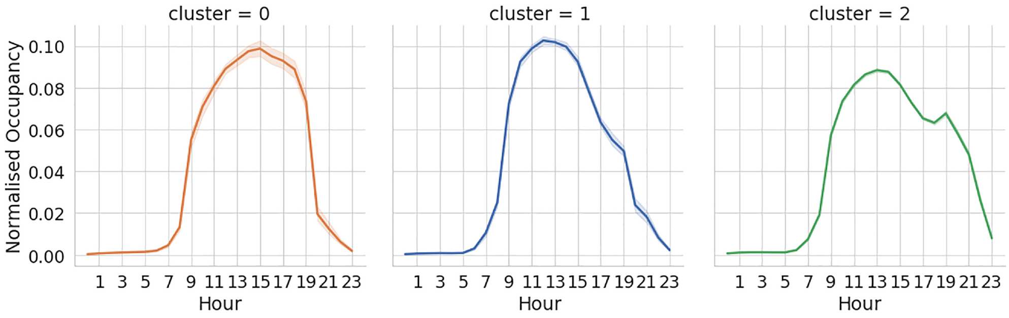
Average occupation as a result of BETAALDP pass parking in hourly intervals from 2016 to 2018 for each cluster group identified by K-means (Euclidean) clustering.

OPEN IN VIEWER

Figure 5.

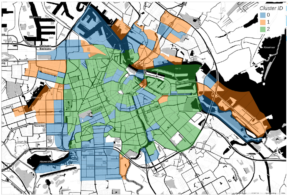
Neighborhood clusters identified by K-means (Euclidean) clustering mapped onto Amsterdam.

Performance of Imputation Models

The aggregated R² and RMSE 5-fold CV mean scores for the city, cluster, and neighborhood training levels are shown in Table 3. The aggregated R² and RMSE 5-fold CV standard deviation scores for various training levels are shown in Table 4. In other words Table 3 communicates the performance that can be expected from the model on unseen data while while Table 4 gives an indication of how stable the the performance is across the CV folds.

OPEN IN VIEWER

Table 3.

Aggregated Scores of the Means of the Root Mean Squared Error (RMSE) and R² Scores Calculated across the 5-Fold Cross Validation (CV) Folds for Various Modeling Methods Trained at Different Levels

Aggregated statistic	Training level	Model type	RMSE score	R2 score
Mean	City	Baseline	0.184	–148.5
		GBM	0.133	–7.89
		RF	0.086	0.081
		LASSO	0.171	–6.42
	Cluster	Baseline	0.173	–114.8
		GBM	0.119	–4.69
		RF	0.086	–0.24
		LASSO	0.166	–97.9
	Neighborhood	Baseline	0.090	–6.89
		GBM	0.087	0.203
		RF	0.088	0.191
		LASSO	0.099	0.003
Standard deviation	City	Baseline	0.00	275.76
		GBM	0.056	39.31
		RF	0.042	1.039
		LASSO	0.171	–6.42
	Cluster	Baseline	0.00	206.5
		GBM	0.053	25.18
		RF	0.042	4.244
		LASSO	0.083	1172.
	Neighborhood	Baseline	0.00	12.87
		GBM	0.041	0.261
		RF	0.042	0.240
		LASSO	0.044	0.089
Median	City	Baseline	0.184	–25.36
		GBM	0.121	–0.34
		RF	0.075	0.201
		LASSO	0.171	–6.42
	Cluster	Baseline	0.173	–24.30
		GBM	0.106	–0.11
		RF	0.076	0.211
		LASSO	0.144	–0.81
	Neighborhood	Baseline	0.090	–1.879
		GBM	0.077	0.226
		RF	0.080	0.199
		LASSO	0.089	–0.00

Note: GBM = gradient boosted method; LASSO = least absolute shrinkage and selection operator; RF = random forest.

OPEN IN VIEWER

Table 4.

Aggregated Scores of the Standard Deviations of the Root Mean Squared Error (RMSE) and R² Scores Calculated across the 5-Fold Cross Validation (CV) Folds for Various Modeling Methods Trained at Different Levels

Aggregated statistic	Training level	Model type	RMSE score	R2 score
Mean	City	Baseline	1598.	0.097
		GBM	0.008	6.343
		RF	0.007	0.303
		LASSO	0.008	31.090
	Cluster	Baseline	1269.	0.091
		GBM	0.008	5.012
		RF	0.007	0.755
		LASSO	0.008	195.4
	Neighborhood	Baseline	90.88	0.045
		GBM	0.007	0.095
		RF	0.006	0.108
		LASSO	0.007	0.025
Standard deviation	City	Baseline	3210.	0.00
		GBM	0.006	38.60
		RF	0.006	1.674
		LASSO	0.006	334.6
	Cluster	Baseline	2382.	0.00
		GBM	0.007	33.78
		RF	0.007	6.064
		LASSO	0.008	2603.
	Neighborhood	Baseline	58.8	0.00
		GBM	0.005	0.102
		RF	0.004	0.115
		LASSO	0.005	0.048
Median	City	Baseline	136.8	0.097
		GBM	0.007	0.132
		RF	0.005	0.076
		LASSO	0.006	0.177
	Cluster	Baseline	241.34	0.091
		GBM	0.007	0.121
		RF	0.005	0.071
		LASSO	0.006	0.180
	Neighborhood	Baseline	31.43	0.045
		GBM	0.005	0.061
		RF	0.005	0.074
		LASSO	0.005	0.009

Note: GBM = gradient boosted method; LASSO = least absolute shrinkage and selection operator; RF = random forest.

The RMSE scores performed very similarly for the GBM, RF, and LASSO methods across all the training levels and metric aggregations. This is interesting, in that the R² metrics vary wildly from method to method for each metric aggregation. The negative R² are of particular concern because it indicates that those models perform worse than using the mean of the data. It should be noted that it is possible to get negative R² values when the predicted values perform worse than the line defined by y i − y ¯ ( y ¯ being the mean), that is, when the fraction is larger than 1 ( 17 ).

The RF method significantly outperforms the other modeling methods at the city and cluster training levels when the median of mean and mean of standard deviation scores are looked at, but it performs similarly (worse) when the mean of mean metrics are looked at. This indicates that the method is performing very poorly for a small subset of neighborhoods which must have extremely bad R² scores. The RF method performs similarly to the gradient boosting machine at the neighborhood training level when the median of means scores are looked at, the respective R² differences being 0.012 and 0.027.

The best training and method combination came from using GBM. It had a mean of mean R² score of 0.2, a median of mean R² score of 0.24, and a standard deviation of mean R² score of 0.24. Figure 6a shows the behavior of these metrics. GBM also obtained a mean standard deviation R² score of 0.095 and a median standard deviation of 0.064. Figure 6b illustrates the behaviors of these last two metrics. The metrics of each distinct model trained per unique neighborhood is represented by the points on Figures 6, a and b ; the colour of each point indicates how many data points were used to train that particular model. The distribution plots of the RMSE and R² scores are illustrated on each respective axis.

OPEN IN VIEWER

Figure 6.

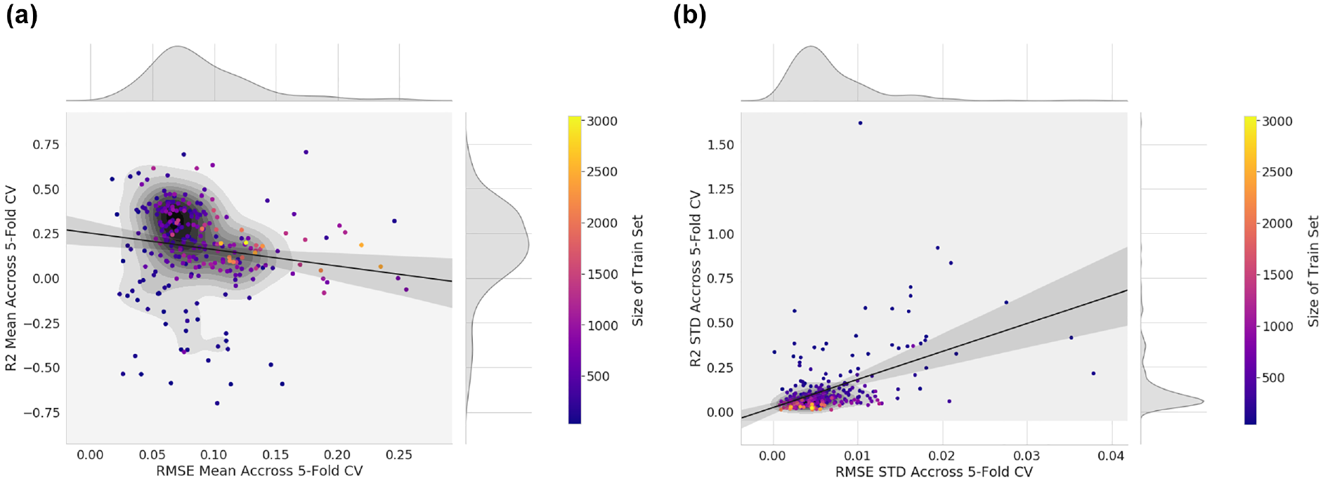
Scatter plot of the R² versus root mean squared error (RMSE) test set metrics from gradient boosted method (GBM) trained at the neighborhood level: (a) Mean of RMSE and R² across 5-fold cross-validation (CV) per neighborhood; (b) Standard deviation of RMSE and R² across 5-fold CV per neighborhood.

The difference in the median and mean R² scores can be explained by the observed long tail distribution in Figure 6a. Furthermore, it can be seen that the individual models built per neighborhood are packed around the median R² score of 0.24, and a large majority are packed around the interval (0.0, 0.5). The individual models achieve very good RMSE scores, tightly packed around 0.08, that is to say, that most of the models are wrong by 8% parking pressure units for their respective neighborhoods.

A weak inverse relationship between RMSE and R² can also be seen in Figure 6a, that is to say, as the models can explain more variance in the data (R²), the lower the RMSE error will be (relative error), but the weakness of this relationship is of concern.

The standard deviation of the RMSE and R² scores for the models that were trained and tested across the 5-folds are shown in Figure 6b. The models achieve very consistent RMSE scores across the 5-folds and deviate by only 0.005. The R² scores, however, are centred around 0.061 and have a more aggressive standard deviation of 0.102. The implication of this is that many individual models for specific neighborhoods will have a different R² score by around 10% parking pressure units.

Given the Structure of the Data, What Supervised Machine Learning Methods Produce the Best Results?

The results indicate that it is possible to impute for parking usage using sparse spatio-temporal parking data from mobile devices with mild confidence by using machine learning methods. In all cases, the GBM and RF models outperformed the baseline models and LASSO models. The LASSO and baseline models were unable to learn the variance of the dependent variable but maintained acceptable RMSE scores.

The best-performing models were the gradient boosting machines trained at the neighborhood level; they achieved mean of mean R² and RMSE scores across all the neighborhoods with 0.203 and 0.087, respectively. Thus, each model per neighborhood is, on average, incorrect by 8% parking pressure units. Likewise, the model is only able to capture roughly 20% of the variance present in the data. What is curious is that the GBM method performs poorly when trained at the city and cluster level, while the RF method radically outperforms it; a possible explanation is because GBM models use an ensemble of weak learners. Thus the GBM method is unable to discriminate the different neighborhoods to make the appropriate prediction, while the RF models can discriminate better what neighborhood to predict for by using the properties of the neighborhood because they are more prone to overfitting.

The low RMSE scores are encouraging in that they indicate that it is indeed possible to use machine learning to impute parking pressure. The R² score indicates that the models are able to explain a small amount of variance, in most cases, around 20%, but this is still several magnitudes better than the baseline model.

Possible explanations for the low variance are that is it a result of the obfuscated ground truth in the data and the bias present in how observations are obtained. The routes that the mobile scanners took were naively constructed and thus did not account for edge cases of false road scans occurring.

There is also the issue of observation bias skewing the ground truth because of the business rules, that is, mobile scanners will drive through areas when they think there might be a high offender rate. This bias also breaks the normally distributed random route assumption made in Bock et al. and might be the leading cause of why the variance is so low ( 4 ). This possible explanation could be further explored by simulating the mobile probe patterns observed in Amsterdam with that of the San Francisco data where there is a better ground truth to validate against ( 8 ).

This paper also did not consider spatial relationships between entities, such as adjacent neighborhood parking pressures and the inter-intra traffic loads. The research by Bock et al. indicates that these features might also better explain the parking pressure, and future work should consider incorporating more spatial relationships between entities ( 4 ).

Can Neighborhood Characteristics of Over-Represented Neighborhoods be Used by Supervised Machine Learning Methods to Better Predict for Under-Represented Neighborhoods?

The results in Table 3 show that the methods trained at the neighborhood level outperform the methods trained with neighborhood properties (the city and cluster levels). This indicates that the methods that were tested are unable to use neighborhood properties to better predict for under-represented neighborhoods. This could be because the methods themselves have their loss functions defined according to the loss of the whole training vector and do not calculate a stratified weighted error. This might create a system that optimises for neighborhood accuracy regardless of the imbalance of training points between neighborhoods.

Do Neighborhoods Show Distinct Parking Behavior and Does the Clustering of these Behaviors Help?

The clustering results showed that three distinct time-series patterns exist and correspond to distinct zones within the city of Amsterdam.

Cluster 0 captures time-series behavior that extends beyond normal work hours, until 7 p.m. This behavior is puzzling because it corresponds to areas that are exclusively high-density apartments: neighborhoods within IJburg, neighborhoods around the inbound highway to the north of Amsterdam, and around Sloterplas. A possible explanation for this is that residents perform errands near their homes after work and thus they use on-street parking on the way home. This could be validated in future work by looking at commuter patterns within these areas.

Cluster 1 captures time-series behavior that corresponds exclusively to business hours. Visual validation of this shows that cluster 1 neighborhoods corresponding to areas that are predominantly business-focused, such as the south and south-west of Amsterdam. Cluster 1 was also able to identify the surrounding areas around the “knowledge highway” (centre east of Amsterdam); this area has a mix of municipal, higher education, and business buildings. Toward the north of Amsterdam, it can also be seen that neighborhoods were classified as cluster 1. These areas also correspond to dense business zones, such as the dockyards, shell corporate offices, and businesses around Sloterdijk Station.

Cluster 2 captures time-series behavior corresponding to behavior that would be expected from mixed-use areas: occupation throughout work hours followed by a decrease as people leave for home, but then a slight increase as people come for the nightlife. Plotting these zones on the Amsterdam geography further validates this assumption because it shows how the neighborhoods belonging to cluster 1 inhabit mixed-use areas of the city with both housing and venues for nightlife, which is a key characteristic of neighborhoods that reside between the highway encircling the city and Old Amsterdam.

The feature importance analysis of the RF method trained at the city level revealed that the identification of cluster 2 was an important feature (top-10 most important) for predicting parking pressure. This could be because cluster 2 overlaps with areas that have low parking pressure peaks due BETAALDP passes (Figure 2) and thus the method uses it to discriminate zones where knowing the BETAALDP passes information is of little influence to the total pressure of that neighborhood.

Policy Application and Data Recommendations

Policymakers traditionally would have to base their decisions on a handful of costly manual counts per neighborhood per year. The imputation of parking offers policymakers the ability to follow time-dynamic trends and to move away from relying on static views of parking usage.

A continuous dynamic parking of pressure view (obtained from the imputed techniques) could allow policymakers to do the following:

The imputation methods are heavily reliant on a good source of historical information on the location and availability of individual parking spots, as this is a prime component of the ground truth. It would be very problematic if this kind of data is not kept up to date, since that will result in matching scans/roads with the wrong locations, and thus wrong parking pressure values.

The ground truth of the scan vehicle data could be enhanced by having a complete GPS trace of a vehicle’s route, as well as a flag indicating whether or not it is scanning for parked cars. Inaccuracies of the GPS coordinates could pose an issue in cities with many high-rises, narrow streets, or overhead trees, and should be considered in future work.

Machine Learning Results

It was found that gradient boosted tree and RF methods outperformed both the average baseline method and the LASSO method. Gradient boosted trees performed the best when models were built for each neighborhood, with an average R² score of 0.20 and RMSE score of 0.087 across all the neighborhoods. Higher R² scores may be achieved if the ground truth of the data is further refined through the use of map matching and historical road networks. This will likely result in improved estimates of the observed parking pressure neighborhood experiences. This analysis may be refined by investigating spatial components through explicit features of adjacent neighborhoods or the use of more advanced deep learning methods as outlined by Yang et al. ( 18 ).

RFs performed the best when compared with alternative methods within the city- and cluster-training-level experiments. The models built using the RF method performed marginally worse (±0.02) than GBM when it was trained at the neighborhood level. The most significant predictors of parking pressure from the best-performing method trained at the city level (RF) were the following; neighborhood characteristics associated with density, buildings associated with leisure, temporal features, and features built from the NPR data.

This paper showed that neighborhood characteristics do not improve the predictive power for under-observed neighborhoods when methods are trained at higher levels of abstraction (cluster and city level). Research in this area may be refined by defining the loss function with respect to a stratification criteria of neighborhoods.

K-means clustering with three clusters was shown to be the best-performing clustering configuration out of the experiments that were conducted. This method identified three unique time-series NPR occupation patterns that corresponded with distinct areas categorised by mixed spaces, work offices, and residential areas. Also, the clustering results help perform imputation when they were used with the RF method trained at the city level. Visual validation indicated that the unique time-series behaviors were independent of the clustering methods used. Further validation could be performed by inspecting properties of the neighborhoods, such as the percentage of building types that exist in each cluster grouping.