Pay Factor Analysis for Highway Pavements through Percentage of Material within Specification Limits and Monte Carlo Simulation

Abstract

Many state highway agencies (SHAs) have adopted pay adjustment provisions in their acceptance plans for construction and materials. In these payment adjustment acceptance plans, the percentage of material within specification limits (PWL) has been selected as the quality measure to relate production quality to pay factors, and pay equations are used to determine a pay factor for a lot based on PWL. Various pay equations have been proposed by the highway community for adoption in SHAs’ specifications. However, the effectiveness of these pay equations has not been fully evaluated. Another issue concerning the pay adjustment acceptance plans is the risk associated with single and multiple pay factors. The purpose of this study was to evaluate the effects of different pay equations commonly used by SHAs and the risks associated with pay adjustment acceptance plans. This was achieved by developing operating characteristic curves associated with various pay factors and expected pay curves and Monte Carlo simulation for assessing the effects in the long run. The methodology suggested in this paper is transferable elsewhere where similar materials and specifications are used for the acceptance of pavements.

Nowadays, the majority of U.S. state highway agencies (SHAs) have adopted the use of pay factors in their acceptance plan for construction and materials. The primary purpose of a pay adjustment provision is to provide sufficient incentives to produce the desired level of quality at the time of initial construction ( 1 ). An effective pay adjustment provision encourages contractors to perform appropriate quality control measures to assure that the finished construction will be equal to or better than the desired quality level most of the time. The secondary objective of the payment adjustment is to recoup at least part of the anticipated future costs of poor quality material or construction ( 1 , 2 ). The percentage of material within specification limits (PWL) has been selected by many SHAs as the quality measure to relate production quality to pay factors. In this situation, many SHAs have defined the acceptable quality level (AQL) and rejectable quality level (RQL) with reference to PWL which is recognized to be an indicator of performance. Today, nearly all SHAs have either developed their pay equations or chosen the method recommended by the American Association of State Highway and Transportation Officers (AASHTO) to determine the pay factor for a given PWL. However, how these pay equations perform in the long term has not been fully evaluated. Furthermore, the majority of the SHAs usually use multiple quality characteristics to determine the pay factor for a lot ( 3 ). To address this issue, this study also deals with the pay factor analysis associated with multiple quality characteristics.

Another issue concerning pay adjustment acceptance plans is the risk associated with single and composite pay factors. Moving away from the accept/reject PWL acceptance plan to the acceptance plan with pay adjustment provision, the evaluation of risks becomes more complex. The concept of α and β risks applied to construction or materials is only appropriate for the case of an accept/reject decision ( 1 , 2 , 4 ). To fully evaluate the risks in the acceptance plans with pay adjustment provision and relate the risks to pay factors, the multiple operating characteristic (OC) curves associated with receiving various pay factors and expected payment curves are necessary. In this study, the multiple OC curves for pay adjustment acceptance plans and expected pay curves are developed by implementing Monte Carlo simulation in MATLAB based on the typical population characteristics from NCHRP Project 10-79: Guidelines for Quality-Related Pay Adjustment Factors for Pavements ( 2 ). These multiple OC curves along with expected pay curves were used to evaluate the long-term performance of different pay equations as well as the risks associated with pay adjustment acceptance plans. While the study draws on the findings of NCHRP Project 10-79 and also FHWA-RD-02-095: Optimal Procedures for Quality Assurance Specifications ( 1 , 2 ), the proposed approach is flexible enough to: (i) accommodate any material and construction quality beyond normal distribution; (ii) consider simulation analysis for generating alternative lots to examine the impact on risks and pay factors in the long run; (iii) incorporate any continuous or stepped pay factor equation desired by a highway agency; and (iv) relate PWL to expected pay and acceptance risks by selecting alternative levels of desired quality indicators. With such flexibility, the inherent constraints of SpecRisk related to the pertinent limitations related to the above points are minimized ( 5 ).

Concepts and Definitions

To fully evaluate the pay equations and the risks associated with pay adjustment acceptance plans, it is necessary to consider their OC curves and expected pay curves. The Transportation Research Board glossary provides the following definitions for the OC curves associated with receiving various pay factors and expected pay curves ( 6 ):

OC curves for payment adjustment acceptance plan: A graphic representation of an acceptance plan that shows the relationship between the actual quality of a lot and the probability of its acceptance at various payment levels.

Expected pay curve: A graphic representation of an acceptance plan that shows the relation between the actual quality of a lot and its expected pay (i.e., mathematical pay expectation, or the average pay the contractor can expect to receive over the long run for submitted lots of a given quality).

Figure 1 shows the typical OC curves associated with various pay factors. It is shown in Figure 1 that each curve illustrates the probability of receiving a pay factor equal to or greater than that demonstrated for the line. For example, an AQL material has an approximately 25% probability of receiving a pay factor equal to or greater than 1.04 and a 64% probability of receiving a pay factor equal to or greater than 1.0. Additionally, it can also be observed that this material has a 100% chance of receiving a pay factor greater than or equal to 0.8. Similarly, the probabilities of receiving various pay factors (i.e., 0.75, 0.9) can also be obtained at any quality level. The α risk, in this case, can be considered as the probability of receiving less than 100% pay for an AQL, while the β risk can be interpreted as the probability of receiving greater than 100% pay, or a pay factor significantly different than that specified, for an RQL material ( 1 , 2 ). However, the use of α and β risks to evaluate the risks is simply not enough. For example, a contractor may be also interested in what is the probability of rejection for an AQL material. Therefore, to fully evaluate the performance of the pay equations and risks, the OC curves associated with receiving various pay factors must be developed.

Figure 1.

Typical operating characteristic curves for pay adjustment acceptance plan.

Pay Equations

As mentioned above, many SHAs have implemented PWL as a quality measure to relate quality (i.e., PWL) to pay factor. Three commonly used pay equations are evaluated by means of OC and expected pay curves. The first pay equation is recommended by AASHTO’s Quality Assurance Guide Specification ( 7 ) while the second pay equation was proposed by Burati et al. ( 1 , 4 ).

PF = 55 + 0.5 \times PWL

(1)

PF = 10 + 1 \times PWL

(2)

The third is a stepped pay equation (Table 1) used by several SHAs for asphalt content, density, and ride quality because it is easy to implement ( 2 ). The step pay equation was developed to produce a similar PWL-PF relation as Equation 1. The concepts of incentives and penalties apply to all pay equations. It can be observed in pay equation 1 that the maximum pay factor will be 105% for a PWL of 100 while the minimum pay factor will be 55% for a PWL of zero. For Equation 2 (“pay equation 2”), the maximum pay factor will be 110% for a PWL of 100 while the minimum pay factor will be 10% for a PWL of zero. However, since most SHA specifications suggest that a 5% incentive payment is adequate, a pay factor of 105% is assigned for any PWL higher than 95 when using pay equation 2. Additionally, there is usually some form of cut off (PF = 0) if the quality level of a lot is below a certain PWL, such as 50 or 60 (RQL). Pay equations 1 and 2 along with different RQLs were used to conduct pay factor analysis. Figure 2 shows the three pay equations graphically with the same RQL of 50. How well these pay equations would perform in practice is examined and evaluated by developing OC and expected pay curves through Monte Carlo simulation.

Table 1.

Stepped Pay Equation (Adapted from NCHRP Project 10-79)

Estimated percentage of material within specification limits	Pay factor (%)
98.0–100	105
94.0–97.9	103
92.0–93.9	101
88.0–91.9	100
84.0–87.9	98
82.0–83.9	96
78.0–81.9	94
74.0–77.9	92
70.0–73.9	90
66.0–69.9	88
62.0–65.9	86
58.0–61.9	84
54.0–57.9	82
50.0–53.9	80
<50.0	0

Figure 2.

Illustration of three different pay equations.

Pay Factor Analysis for Single Quality Characteristic

Monte Carlo simulations were conducted in MATLAB to develop OC curves associated with receiving various pay factors and expected pay curves ( 8 – 10 ). The population distributions (means and standard deviations shown in Table 2) are shifted to produce different PWLs. Each PWL represents the quality level of a simulated lot, and the simulated lots have the same standard deviation as the population distribution. The three pay equations were then used to calculate the pay factors for each simulated lot. The probabilities of receiving greater than or equal to various pay factors (i.e., 0.7, 0.8, 0.9, 1.0, 1.04) for a specific PWL can be determined as follows, where PF is pay factor.

Probability of receiving \geq PF = \frac{number of lots \geq PF}{Total number of lots}

Table 2.

Means, Standard Deviations and Specification Limits for Different Quality Characteristics (Adapted from NCHRP Project 10-79)

Quality characteristics	Strength (psi)	Thickness (in.)	Roughness (in./mile)
Standard deviation	509.90	0.54	8.69
Average	4536.00	12.10	59.69
Specification limit	LSL = 3500	LSL = 11.2, USL = 12.8	USL = 75

Note: LSL = lower specification limit; USL = upper specification limit.

OC curves for several specified payment levels (0.7, 0.8, 0.9, 1.0, 1.04) were plotted for concrete strength, thickness, and roughness representing the population distribution.

OC Curves for Pay Adjustment Acceptance Plans

The OC curves shown in Figure 3 were developed using the population standard deviation of concrete strength based on pay equation 1. The probability values of receiving equal to or greater than various pay factors (i.e., 0.7, 0.8, 0.9, 1.0 and 1.04) are shown in Table 3. It can be seen that the probability of receiving a pay factor greater than or equal to 1.0 is 2.83% for RQL of 50 quality level while the chance of receiving a pay factor greater than or equal to 1.0 is 60.84% for AQL of 90. This indicates that there is an approximately 40% probability that a contractor would not receive full payment (100%) for an AQL production, which represents a very high risk for a PF = 1.0 curve. However, it is somehow balanced by the fact that there is a more than 40% chance of receiving a pay factor of 1.04 or greater indicated by the PF = 1.04 curve ( 1 ). Similarly, the probability of receiving greater than or equal to various pay factors (i.e., 0.7, 0.8, 0.9, 1.0 and 1.04) for any quality levels can be estimated using Figure 3.

Figure 3.

Operating characteristic curves using pay equation 1 and n = 5 for strength population.

Table 3.

Probability of Receiving Greater than or Equal to Pay Factor for Pay Equation 1 and n = 5

PWL	Probability of receiving ≥ pay factor
PWL	0.7	0.8	0.9	1.0	1.04
0	0.00	0.00	0.00	0.00	0.00
10	0.18	0.18	0.00	0.00	0.00
20	3.00	3.00	0.24	0.02	0.02
30	13.00	13.00	2.06	0.31	0.12
40	29.40	29.4	6.32	1.09	0.57
50	50.00	50.00	14.88	2.83	1.12
60	70.00	70.00	28.49	7.14	3.33
70	86.94	86.94	50.12	15.80	8.48
80	96.92	96.92	75.15	32.36	18.96
90	99.85	99.85	94.14	60.84	40.96
100	100.00	100.00	100.00	100.00	100.00

Note: PF = pay factor; PWL = percentage of material within specification limits.

PF = 0 if PWL < 50.

10,000 simulated lots.

OC Curves for Different Pay Equations

Table 4 summarizes the probability of receiving greater than or equal to various pay factors from simulation analysis, while Figure 4 shows the OC curves for the pay adjustment acceptance plan using pay equation 2. Overall, the OC curves in Figure 4 became less spread to each other compared with the OC curves in Figure 3. The PF = 1.0 curve in Figure 4 is very similar to that in Figure 3. However, compared with the OC curves using pay equation 1 (Figure 3), the probabilities of receiving a pay factor equal to or larger than 1.04 (PF = 1.04 curve) increase for any given PWL, while the probabilities of receiving a pay factor larger than 0.7, 0.8 and 0.9 decrease. For example, it is shown in Figure 4 that the probability is approximately 50.8% (compared with 40% in Figure 3) for an AQL material to receive 104% pay, while the probability is approximately 81% (compared with 90.4% in Figure 3) for an AQL material to receive 90% pay. This indicates that using pay equation 2 increases the spread of pay factor estimates.

Table 4.

Probability of Receiving Greater than or Equal to Pay Factor for Pay Equation 2 and n = 5

PWL	Prob. of receiving ≥PF
PWL	0.7	0.8	0.9	1.0	1.04
0	0.00	0.00	0.00	0.00	0.00
10	0.06	0.01	0.00	0.00	0.00
20	0.87	0.23	0.07	0.04	0.03
30	5.50	1.80	0.60	0.27	0.15
40	14.7	6.06	2.50	0.93	0.59
50	30.89	14.25	6.16	2.75	1.93
60	50.55	29.34	14.87	6.63	4.65
70	73.10	50.71	29.90	15.87	11.80
80	90.79	74.92	52.65	31.41	24.60
90	99.07	94.6	81.4	60.25	50.85
100	100.00	100.00	100.00	100.00	100.00

Note: PF = pay factor; PWL = percentage of material within specification limits.

PF = 0 if PWL < 50, PF = 105 if PF > 105.

10,000 simulated lots.

Figure 4.

Operating characteristic curves using pay equation 2 and n = 5 for strength population.

The stepped pay equation (Table 1) was used to developed multiple OC curves through simulation analysis. Table 5 summarizes the probability of receiving greater than or equal to various pay factors while Figure 5 shows the OC curves for the pay adjustment acceptance plan developed using population characteristics of concrete strength based on the stepped pay equation and a sample size of five. Overall, the OC curves shown in Figure 5 are very similar to the OC curves in Figure 3 except that the probabilities of receiving 100% pay (PF = 1 curve) for any PWLs in Figure 5 are slightly larger than those in Figure 3. This means that these pay equations produce similar expected pay in the long term.

Table 5.

Probability of Receiving Greater than or Equal to Pay Factor Based on Stepped Pay Equation and n = 5

PWL	Probability of receiving ≥PF
PWL	0.7	0.8	0.9	1.0	1.04
0	0.00	0.00	0.00	0.00	0.00
10	0.43	0.43	0.02	0.00	0.00
20	3.22	3.22	0.13	0.00	0.00
30	13.33	13.3	1.77	0.33	0.07
40	28.97	28.97	6.18	1.30	0.51
50	49.72	49.72	15.1	3.33	1.27
60	70.02	70.02	29.00	8.10	3.32
70	87.10	87.10	51.01	18.08	8.46
80	97.02	97.02	75.21	35.64	18.91
90	99.85	99.85	95.69	65.09	41.06
100	100.00	100.00	100.00	100.00	100.00

Note: PF = pay factor; PWL = percentage of material within specification limits.

PF = 0 if PWL < 50.

10,000 simulated lots.

Figure 5.

Operating characteristic curves using stepped pay equation and n = 5 for strength population.

EP Curves for Different Pay Equations

The OC curves enable evaluation of the risks involved in the pay adjustment acceptance plans. However, using such OC curves is not a simple way to evaluate the overall pay performance of an acceptance plan. To fully evaluate and compare the overall pay performance of the three different pay equations, it is necessary to develop expected pay curves. Table 6 summarizes the average pay factors for various quality levels from simulation analysis, while Figure 6 shows the expected pay curves of the three pay equations for a sample size of five.

Table 6.

Expected Payments in Relation to PWL for Three Pay Equations.

PWL	Average pay factor (%)
PWL	(1)	(2)	Stepped
100	105.00	105.00	105.00
90	100.00	98.08	100.00
80	93.00	87.50	92.12
70	80.00	73.20	80.67
60	63.00	55.00	64.45
50	43.00	37.80	42.93
40	25.50	21.00	23.35
30	11.40	10.00	10.25
20	2.50	1.90	2.65
10	0.15	0.15	0.36
0	0.00	0.00	0.00

Note: PF = pay factor; PWL = percentage of material within specification limits.

PF = 0 if PWL < 50.

10,000 simulated lots.

Figure 6.

Expected pay curves for different pay equations and n = 5.

It can be seen in Figure 6 that the expected pay curves for pay equation 1 and the stepped pay equation are essentially identical. The expected pay for AQL materials using pay equation 1 and stepped pay schedule is 100%, however, only 98.08% payment for an AQL material was obtained using pay equation 2. Thus it can be concluded that pay equation 2 results in a larger pay risk to the contractor.

Effects of Sample Size

To analyze the effects of sample size on the probability values of receiving various pay factors, another sample size of 15 was used to develop the OC curves. The probabilities of receiving greater than or equal to various pay factors using the strength population and pay equation 1 for a sample size of 15 are plotted in Figure 7. Overall, the OC curves shown in Figure 7 (n = 15) are more spread compared with the OC curves in Figure 3 (n = 5). It can also be seen that an AQL (PWL = 90) quality level has an 8.69% chance of receiving a pay factor equal or greater than 1.04 and a 100% probability of receiving a pay factor equal or greater than 0.9. This means that the distribution of pay factors using a sample size of 15 is much more centered at PF = 1.0 than that using a sample size of five.

Figure 7.

Operating characteristic curves using pay equation 1 and n = 15.

The expected payment curves are developed to represent the long-term pay performance. Figure 8 shows the expected pay in relation to PWL for sample sizes of five and 15 using pay equation 1. It can be seen in Figure 8 that the expected pay curve becomes steeper with the increase of sample size. This indicates that as the sample size increases, the expected pay decreases faster as the PWL reduces ( 11 ). The average pay factor is 100% for an AQL of 90 for both sample sizes of five and 15. For a PWL of 80, the average pay factor is 95.0% for a sample size of 15 and 93.0% for a sample size of five. However, for a poor quality level (PWL = 40), the average pay factor is 13.8% for a sample size of 15 and 25.5% for a sample size of five, respectively. This is because as the sample size increases a better estimation of the population characteristic can be obtained.

Figure 8.

Expected pay curves using pay equation 1 for n = 5 and 15.

Effects of RQL

The expected pay values in relation to PWLs using pay equation 1 with different RQLs (i.e., 40, 50 and 60) are summarized in Table 7 and plotted in Figure 9. Overall, it is shown in Figure 9 that the average pay factor decreases, as expected, with the increase of RQL from 40 to 60. Changing the RQL from 50 to 60 does not have a significant impact on the average pay factor for the AQL material. For example, the average pay factor is 99.3% for an AQL with RQL of 60, while the average pay factor increases to 100% for an AQL using the same pay equation with RQL of 40. This also indicates that the pay risk for contractors using pay equation 1 with an RQL of 60 is higher than that with an RQL of 40. However, for a poor quality level (i.e., PWL = 50), it also should be noticed that the pay risk for agencies using pay equation 1 with an RQL of 60 is lower than that with an RQL of 40. Therefore, such analysis should be performed by SHAs to determine a reasonable RQL to balance the risks to agencies and contractors.

Table 7.

Expected Pay in Relation to PWL Based on Pay Equation 1 and n = 5

PWL	Average pay factor (%)
PWL	40	50	60
100	105.0	105.0	105.0
90	100.0	99.9	99.3
80	94.6	93.1	87.4
70	86.7	80.5	68.6
60	76.2	63.2	46.8
50	60.1	43.3	27.1
40	42.9	25.5	13.7
30	25.8	11.4	5.0
20	8.4	2.5	0.7
10	1.2	0.2	0.0
0	0.0	0.0	0.0

Note: PWL = percentage of material within specification limits.

Figure 9.

Expected pay curves using pay equation 1 and n = 5 for different rejectable quality levels (RQL).

Pay Factor Analysis for Multiple Quality Characteristics

The pay factor analyses above are based on a single quality characteristic. However, SHAs more often use multiple quality characteristics to determine the pay factor for a lot. There are two different ways to calculate the pay factors associated with multiple quality characteristics. The first approach is using a weighting system to combine individual PWL and calculate a composite PWL (CMPWL) as shown in Equation 3. The composite pay factor CMPF₍₁₎ is then determined based on CMPWL using Equation 4 (“pay equation 4”, derived from pay equation 1) or CMPF₍₂₎, based on Equation 5 (“pay equation 5”, derived from pay equation 2). Similarly, a CMPF of 105% is assigned for any CMPWL larger than 95 when using pay equation 5. The more important quality characteristics would be assigned a larger weighting.

\begin{matrix} CMPWL = 0.25 \times PW L_{strength} + 0.35 \times PW L_{thickness} \\ + 0.4 \times PW L_{roughness} \end{matrix}

(3)

where

PWL_strength = percent within specification limit for strength

PWL_roughness = percent within specification limit for roughness

PWL_thickness = percent within specification limits for thickness

CMP F_{(1)} = 55 + 0.5 \times CMPWL

(4)

CMP F_{(2)} = 10 + 0.5 \times CMPWL

(5)

It should be noted that, to differentiate it from the composite pay factor calculated using Equation 6 below (“pay equation 6”), CMPF is used here to represent the composite pay factor calculated based on CMPWL. The second method was recommended by NCHRP Project 10-79 ( 2 ) and is widely used by SHAs across the country. This method suggests that the pay factors for individual characteristics should be calculated first using pay equation 1 or 2, then composite pay equation 6 will be used to combine the individual pay factors to calculate the composite pay factor (CPF).

\begin{matrix} CPF = 0.25 \times P F_{strength} + 0.35 \\ \times P F_{thickness} + 0.4 \times P F_{roughness} \end{matrix}

(6)

where

PF_strength = pay factor for strength

PF_roughness = pay factor for roughness

PF_thickness = pay factor for thickness

Pay equations 3 and 6 may produce different pay factors because different combinations of individual PWL may produce the same composite quality level (CMPWL). For example, two hypothetical lots are shown in Table 8. Lot 1 and lot 2 have the same CMPWL of 90%, however, the PWLs of each individual characteristic are different. Equation 6 produces a pay factor of 100% for lot 1, while pay equation 3 provides a pay factor of 94.9%.

Table 8.

Lots with Different Combinations of PWL Producing CMPWL of 90%

Quality characteristic	PWL for Lot 1 (%)	PWL for Lot 2 (%)
Strength	60	90
Thickness	100	90
Roughness	100	90
CMPWL	90	90
Pay factor based on CMPWL (CMPF)	100	100
Composite pay factor (CPF)	94.9	100

Note: PWL = percentage of material within specification limits; CMPWL = composite PWL.

Figure 10 shows the flow chart of conducting pay factor analysis for multiple quality characteristics using two different methods. Both methods were used to develop the OC curves for multiple quality characteristics. The CMPWLs were calculated based on Equation 3. It should be noted that a certain CMPWL could be obtained from different combinations of PWLs for each parameter. However, in this analysis, the same PWL for individual characteristics is used to produce a certain level of CMPWL. For example, a CMPWL of 90% is obtained when every single PWL is at AQL of 90.

Figure 10.

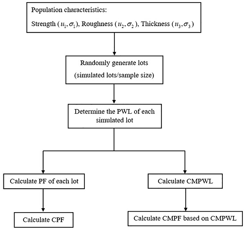
Flow chart of pay factor analysis for multiple quality characteristics.

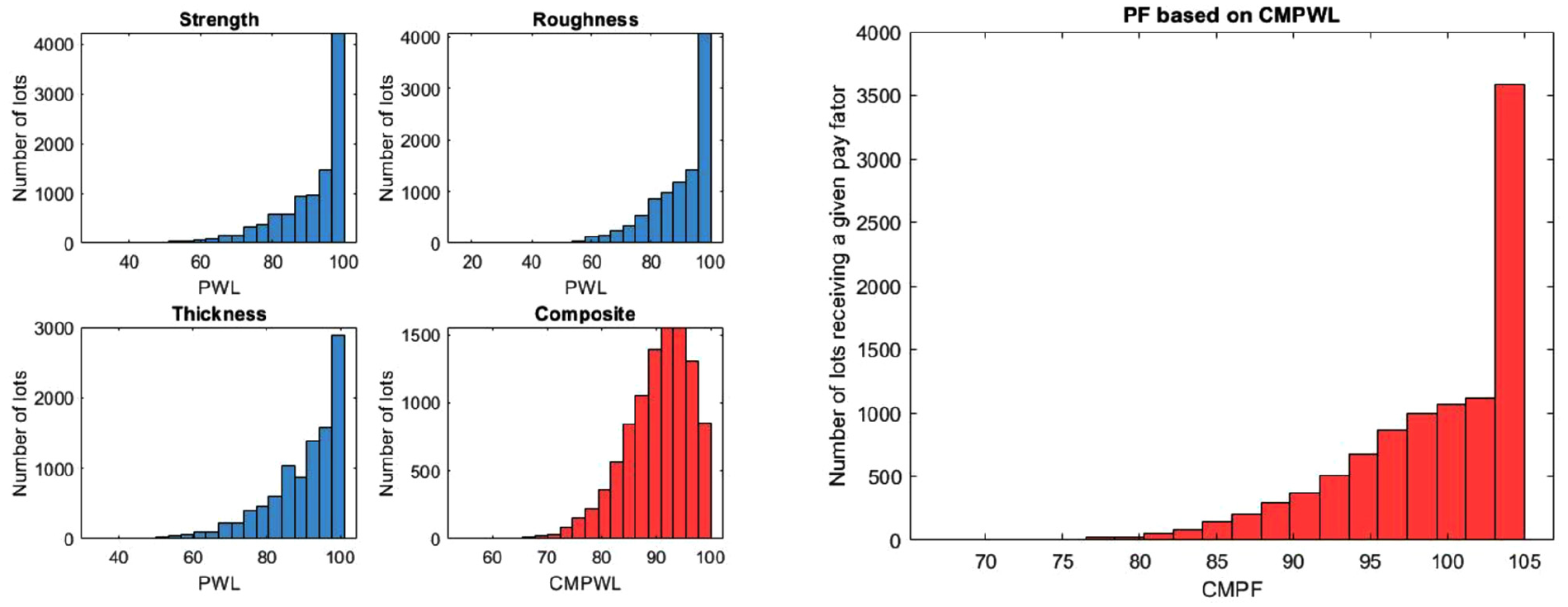
As in the previous analysis, the population distributions for each quality characteristic (strength, thickness, and roughness) were shifted to produce different PWLs. Then pay equation 3 was applied to calculate the CMPWL of the lots, and the CMPF was determined by pay equation 4 or 5. Table 9 summarizes the probability values of receiving greater than or equal to various CMPFs using pay equation 4 while Figure 11 shows the OC curves based on CMPWL and CMPF. It is shown in Table 9 that the probability of receiving CMPF greater than or equal to 1.0 is 0% for RQL (CMPWL = 50) while the chance of receiving CMPF greater than or equal to 1.0 is 57.78% for AQL (CMPWL = 90). Overall, the OC curves (Figure 11) developed based on multiple quality characteristics are more spread than that developed based on a single quality characteristic (Figure 3), indicating that the dispersion of CMPWL and CMPF estimates are smaller than that of PWL and pay factor estimates. This can also be demonstrated by the histogram for an AQL population showing the variability of PWL, CMPWL, and CMPF in Figure 12. The standard deviation of the estimated PWLs for a single characteristic was approximately 11.0 for a sample size of five, while the standard deviation was calculated to be 6.34 for CMPWLs and 3.17 for CMPF, respectively. This is because many individual PWLs were randomly combined, leading to a balancing out between high and low PWLs such that the CMPWL was more centered to 90.

Table 9.

Probability of Receiving Greater than or Equal to CMPF Using Pay Equation 4 and n = 5

CMPWL	Probability of receiving ≥CMPF
CMPWL	0.7	0.8	0.9	1.0	1.04
0	0.00	0.00	0.00	0.00	0.00
10	0.00	0.00	0.00	0.00	0.00
20	0.15	0.15	0.00	0.00	0.00
30	2.72	2.72	0.00	0.00	0.00
40	17.02	17.02	0.18	0.00	0.00
50	50.66	50.66	2.52	0.00	0.00
60	84.73	84.73	17.55	0.06	0.00
70	98.25	98.25	54.55	1.07	0.00
80	99.92	99.92	88.48	11.47	0.32
90	100.00	100.00	99.62	57.78	7.83
100	100.00	100.00	100.00	100.00	100.00

Note: PF = pay factor; PWL = percentage of material within specification limits; CMPWL = composite percentage of material within specification limits; CMPF = composite pay factor calculated from CMPWL.

PF = 0 if PWL < 50.

10,000 simulated lots.

Figure 11.

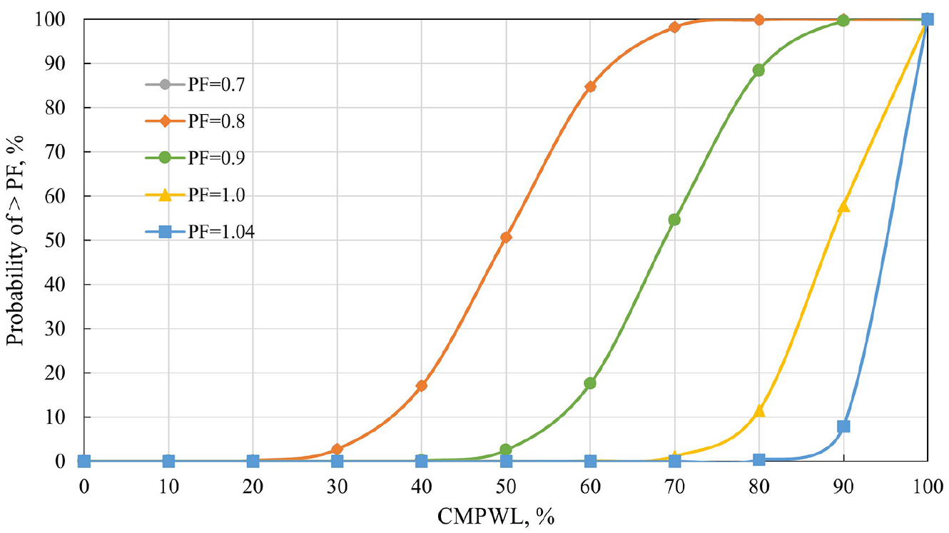
Operating characteristic curves using pay equation 4 and n = 5.

Figure 12.

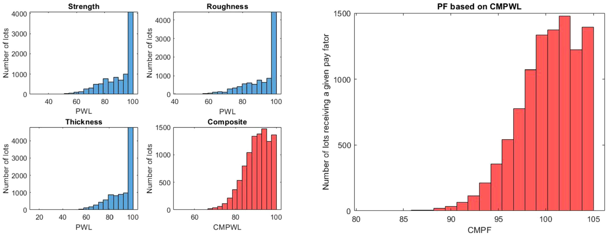
Acceptable quality level population showing the variability of CMPWL and CMPF for pay equation 4 and n = 5.

The OC curves were then developed using pay equation 5 for the same sample size of five. The results were summarized in Table 10 and plotted in Figure 13. For an AQL material, the same average CMPF of 100% was obtained based on pay equations 4 and 5, however, the probabilities of receiving CMPF greater than or equal to various pay factors (i.e., 0.7, 0.8, 0.9, 1.0 and 1.04) and OC curves are different. For example, the probability of receiving CMPF greater than or equal to 1.04 was estimated to be 7.83% based on pay equation 4, while this probability changed dramatically to 31.2% for an AQL based on equation 5. This indicates that if equation 5 were used, the contractor would tend to receive more incentive pay for an AQL since more simulated lots receive a pay factor larger than 1.04 as for the case of pay equation 4. Figure 14 provides the histogram for an AQL population showing the variability of CMPWL and CMPF based on pay equation 5. Compared with Figure 12, a much larger variability (standard deviation estimated to be 5.5) for CMPF was observed.

Table 10.

Probability of Receiving Greater than or Equal to CMPF Using Pay Equation 5 and n = 5

CMPWL	Probability of receiving ≥CMPF
CMPWL	0.7	0.8	0.9	1.0	1.04
0	0.00	0.00	0.00	0.00	0.00
10	0.00	0.00	0.00	0.00	0.00
20	0.00	0.00	0.00	0.00	0.00
30	0.15	0.01	0.00	0.00	0.00
40	2.75	0.20	0.01	0.00	0.00
50	16.63	2.55	0.12	0.00	0.00
60	50.52	16.44	2.08	0.06	0.01
70	86.62	53.38	16.22	1.12	0.22
80	98.61	88.08	54.49	11.65	3.48
90	99.97	99.47	93.7.	57.28	31.20
100	100.00	100.00	100.00	100.00	100.00

PF = 0 if PWL < 50, PF = 105 if PF > 105.

10,000 simulated lots.

Figure 13.

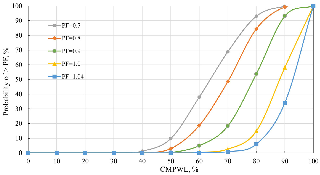
Operating characteristic curves using pay equation 5 and n = 5.

Figure 14.

Acceptable quality level population showing the variability of CMPWL and CMPF for pay equation 5 and n = 5.

The above pay factors were determined using CMPWL while the following pay factor analysis was based on the composite pay equation (Equation 6) used to determine CPF, which combines the pay factors of individual quality characteristics. As shown in Figure 10, the pay factor of the simulated lots for a single quality characteristic can be calculated using pay equation 1 or 2, and then the CPFs can be determined using pay equation 6. The OC curves for multiple quality characteristics using pay equation 1 combined with pay equation 6 were developed. The results are summarized in Table 11 and plotted in Figure 15. It can be observed from Table 11 that the probability values of receiving CPF greater than or equal to 1.04 and 1.0 are calculated to be approximately 10.91% and 55.23%, respectively, while the probabilities of receiving CMPF greater than or equal to 1.04 and 1.0 are calculated to be approximately 7.83% and 57.0%.

Table 11.

Probability of Receiving Greater than or Equal to CPF Using Pay Equations 1 and 6 and n = 5

CMPWL	Probability of receiving ≥CMPF
CMPWL	0.7	0.8	0.9	1.0	1.04
0	0.00	0.00	0.00	0.00	0.00
10	0.00	0.00	0.00	0.00	0.00
20	0.00	0.00	0.00	0.00	0.00
30	0.09	0.09	0.00	0.00	0.00
40	1.56	1.56	0.17	0.00	0.00
50	12.23	12.12	2.60	0.01	0.00
60	41.26	40.96	19.16	0.37	0.02
70	70.18	69.42	48.51	2.55	0.13
80	92.14	91.44	83.81	14.92	1.36
90	99.68	99.45	99.12	55.23	10.91
100	100.00	100.00	100.00	100.00.	100.00

PF = 0 if PWL < 50.

n = 5, 10,000 simulated lots.

Figure 15.

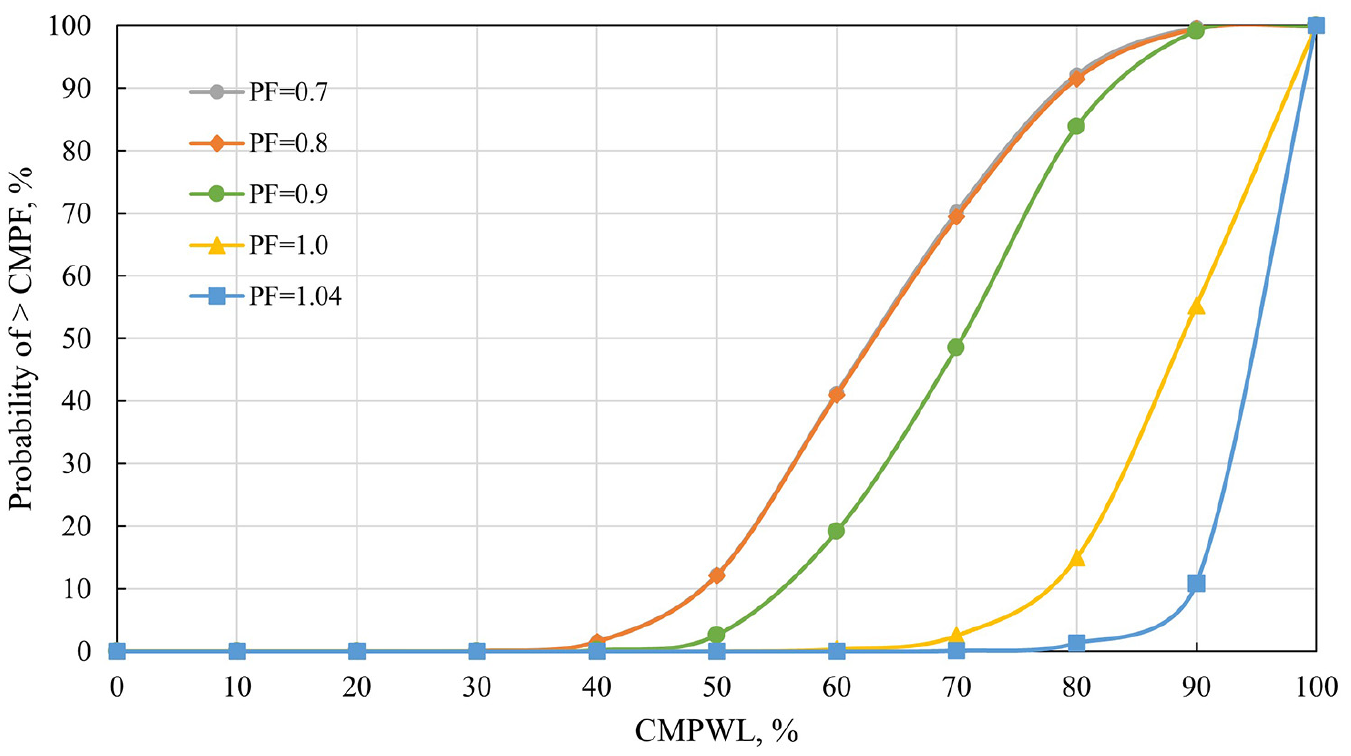
Operating characteristic curves using pay equations 1 and 6 and n = 5. PF = 0.7 and PF = 0.8 curve values overlap.

For an AQL, average pay factor is calculated to be 100% for both CPF and CMPF. This indicates that the two methods of pay factor analysis for multiple quality characteristics provide similar results for the AQL population. However, for a CMPWL of 80, the average CMPF was calculated to be 95.3% while the average CPF was determined to be 93.1%. This indicates that, for multiple quality characteristics, using CMPWL to calculate the pay factor provides a larger CPF. It fails to apply a cut off (i.e., PF = 0 if PWL < 50) for individual quality characteristics such that the pay factor for a lot may be overestimated.

Conclusions and Recommendations

The OC and expected pay curves for pay adjustment acceptance plans were developed using Monte Carlo simulation for both single and multiple quality characteristics to evaluate the risks and associated pay factors. The effects of sample size and RQL on the contractor and agency risks were also analyzed in conjunction with the associated pay factors.

The pay factor analysis shows that:

As expected, increasing RQL will increase the probability of awarding lower pay to the contractors, as well as reduce the average pay factors in the long run.

Increasing the sample size from five to 15 has no significant impact on the average pay factor when an AQL of 90 is considered. However, this impact becomes more significant when the production quality (PWL) drops. As expected, increasing sample size provides a better inference of the true population characteristics. These trends are in agreement with the findings from past studies.

The three alternative pay equations (i.e., continuous pay equations 1 and 2, and stepped pay equation) provided the same overall average pay factor (i.e., 100% pay) for production with an AQL of 90 and when an RQL of 50 is considered with a sample size of five. The continuous pay equation 1 and the stepped pay equation produce similar expected pay, while pay equation 2 provides relatively low expected pay for PWLs lower than AQL of 90.

When using multiple quality characteristics to determine the pay factor for a lot, instead of using the composite percent within limits to calculate the composite pay factor, it is suggested that the pay factor for individual quality characteristics should be determined first and then a weighting system be applied to calculate the composite pay factor. The methodology suggested in this research can be applied elsewhere for assessing relating risks and pay factors for the acceptance of pavements.

Footnotes

Author Contributions

The authors confirm contribution to the paper as follows: study conception and design: D. Goulias, Y. Zhao; data collection: Y. Zhao, D. Goulias; analysis and interpretation of results: Y. Zhao, D. Goulias; draft manuscript preparation: Y. Zhao, D. Goulias. Both authors reviewed the results and approved the final version of the manuscript.

Declaration of Conflicting Interests

The author(s) declared no potential conflicts of interest with respect to the research, authorship, and/or publication of this article.

Funding

The author(s) received no financial support for the research, authorship, and/or publication of this article.

ORCID iD

Yunpeng Zhao

References

Burati

Weed

Hughes

Hill

Optimal Procedures for Quality Assurance Specifications. Report FHWA-RD-02-095. Federal Highway Administration, Washington, D.C., 2017.

Hughes

C. S.

Moulthron

J. S.

Tayabji

Weed

R. M.

Burati

J. L.

Guidelines for Quality-Related Pay Adjustment Factors for Pavements. National Cooperative Highway Research Program 10-79. Transportation Research Board of the National Academies, Washington, D.C., 2011.

Burati

Risks with Multiple Pay Factor Acceptance Plans. Transportation Research Record: Journal of the Transportation Research Board, 2005. 1907: 97–42.

Burati

Weed

Hughes

Hill

Evaluation of Procedures for Quality Assurance Specifications. Report FHWA-HRT-04-046. Federal Highway Administration, McLean, VA, 2004.

Weed

R. M.

Quality Assurance Software for the Personal Computer. Publication No. FHWA–SA–96–026. Federal Highway Administration, Washington, D.C., 1996.

Transportation Research Circular No. E-C235: Glossary of Highway Quality Assurance Terms . Transportation Research Board, Washington, D.C., 2018.

Standard Practice for Definition of Terms Related to Quality and Statistics as Used in Highway Construction. AASHTO Designation R 10-06. In Standard Specifications for Transportation Materials and Methods of Sampling and Testing, Part I Specifications, 33rd ed. American Association of State Highway and Transportation Officials, Washington, D.C., 2018.

Karimi

Goulias

Schwartz

Risk and Expected Pay Factor Analysis for Assessing Gap and Dense-Graded Superpave Mixture Specification. International Journal of Pavement Engineering, Vol. 16, No. 1, 2015, pp. 69–79.

Zhao

Goulias

Evaluation of Acceptance Risks through Percent within Limit for Highway Materials and Pavement Construction. Transportation Research Record: Journal of the Transportation Research Board, 2021. https://doi.org/10.1177/03611981211006436

10.

Goulias

Schwartz

Karimi

Hughes

Increasing Durability of Hot Mix Asphalt Pavements Designed with the Superpave System. Research Report MD-SP708B4E. Maryland Department of Transportation State Highway Administration, Office of Materials and Technology, Hanover, 2009.

11.

Villiers

Mehta

Lopp

Tia

Roque

Evaluation of Percent-within-Limits- Construction Specification Parameters. International Journal of Pavement Engineering, Vol. 4, No. 4, 2003, pp. 221–228.