A Deep Learning Model for Off-Ramp Hourly Traffic Volume Estimation

Abstract

This paper addresses estimation of traffic volume of freeway off-ramps. Freeways are the transportation network’s main corridors, serving a large portion of the traffic volume. This traffic passes into the lower-level roads through off-ramps. Therefore, the traffic condition of the off-ramps is an essential factor affecting the operation of the transportation network. The continuous collection of volume data is impractical, and transportation authorities install vehicle detectors permanently on only a few off-ramps and temporarily (e.g., a week) on some others. Thus, traffic volume is the most challenging to estimate among various traffic measures. Moreover, the existing literature on volume estimation is mainly concerned with evaluating traffic on the main road segments. However, the distinct characteristics of the connection links, such as off-ramps, demands specified modeling. This study estimates the hourly traffic volume of off-ramps using a deep learning model. It evaluates the advantages of inputting the connected lower-level road features to the model, and explores various detector installation strategies on the model training process. The primary data sources are volume counts, probe speeds, and road segment infrastructure characteristics. The model results indicate that the incorporation of traffic flow characteristics and infrastructure attributes of the lower-level road connected to the freeway significantly improves the accuracy of estimation off-ramp traffic volume. Further, analysis illustrated that the model trained with data from temporarily installed detectors on all interchanges outperformed models trained with permanently installed detectors on 90% of the interchanges, indicating the model’s ability in extracting temporal correlations significantly more than spatial correlations.

The aim of this study is to improve estimation of the number of vehicles that exit a freeway in an hour and enter the arterials using traffic counts data. As the backbone of a road network, freeways are the essential corridors determining the entire network’s traffic conditions. The interaction of freeways and the rest of the road network is through on- and off-ramps. The large volume of traffic that uses the freeways must use off-ramps to go to lower-level roads and arrive at their destination. The amount of traffic that exits a freeway, especially during peak hours, can create traffic congestion, thereby severely affecting the performance of downstream roads. The drop in road performance occurs because the design of arterials and collectors is adequate for a much lower traffic volume than freeways. Contrary to other road segments that typically have a high-resolution speed record as an indicator of the traffic volume, such records are not available for on- and off-ramps because they do not have a traffic messaging channel (TMC) segment designated to them. This study’s motivation is to provide a framework for the system operators to estimate and predict the traffic volume that exits a freeway and enters the local roads to plan accordingly.

The traditional method for estimating link flows relies on traffic assignment techniques. These techniques aim to compute link flows based on the origin–destination (OD) matrix and equilibrium assumptions ( 1 ). Therefore, the OD matrix is a critical element in the process of estimating link flows. Many studies focus on OD matrix estimation models and can be categorized into two groups: static and dynamic-based models ( 2 ). Static models yield an average OD matrix, which is time-independent and is useful for planning level flow estimations. At the same time, dynamic methods aim to estimate the time-dependent OD matrix to be used at the operational level ( 3 – 6 ). Most of the studies in this area have an outdated OD matrix as input and aim to update that matrix using time-varying traffic counts ( 7 ). The modified OD matrix is then inputted into a dynamic traffic assignment (DTA) model to obtain link flows. There exist a wide range of DTA models which also can be categorized into two classes: analytical and simulation-based. Interested readers may refer to Peeta and Ziliaskopoulos ( 8 ) for more details on these models.

One other way to approach the link flow estimation problem is through macroscopic traffic flow modeling. These models mainly aim to estimate various traffic state variables—namely, flow, mean speed, and density—using data assimilation techniques such as the Kalman filtering or its variations, such as extended Kalman filter ( 9 ). While these models may provide acceptable estimations in a range of applications, for instance, in traffic speed estimation ( 10 ), travel time estimation ( 11 , 12 ), traffic volume estimation ( 13 ), and autonomous vehicle driving ( 14 – 18 ), their accuracy in capturing the dynamic patterns of traffic flow are debatable. In recent years, advancements in machine learning-based methods, as well as the availability of large-scale datasets such as probe vehicle data ( 19 ), have provided the opportunity to approach the link flow estimation problem from another aspect. Various machine learning-based models, such as support vector regression ( 20 ), random forest ( 21 ), neural networks ( 22 ), among others, are utilized to estimate link flows. Several studies have illustrated the superior performance of neural network models in estimating various road traffic characteristics ( 23 – 28 ).

Despite the evident importance of freeway ramps flow, investigating this variable as a stand-alone problem is overlooked in the transportation literature ( 29 ). While there are methodologies for estimating networkwide hourly traffic volume, their application for estimation of ramp volume is limited. These methods generally require a high-resolution speed profile as input ( 23 , 30 ), which is not available for most ramps without a designated TMC segment.

This study trains neural network models to estimate traffic flow on freeway exits (i.e., off-ramps). An accurate estimation of the traffic counts on freeway ramps is beneficial from two points of view. Firstly, the information on exiting vehicle counts can greatly benefit traffic management systems to alleviate traffic congestion in the road network. Secondly, ramp flows, which are an indicator of the traffic’s general movement, can be added as a valuable input to the OD matrix estimation models if estimated accurately. While the introduced methodology can be modified to be applied to other connection links such as on-ramps, only off-ramps are considered in this study to leave room for analyzing the spatio-temporal nature of off-ramp flows. These analyses are conducted considering two perspectives. The first focuses on the effects of several spatial features on the performance of the trained models. The second explores the impact of the ground truth volume data on accuracy of estimation of off-ramp flows. This analysis is performed through training two models based on different strategies that exist for volume data collection. The current study findings benefit the transportation network operators since it provides them with a model framework while investigating the required input data and data collection strategies for off-ramp hourly traffic volume estimation.

The rest of this paper is organized as follows. First, an overview of the data sources used in this study is provided. Afterward, the methodology used to estimate off-ramp hourly traffic volume is explained. This explanation of the methodology is followed by a section comparing the introduced method’s performance under various scenarios to analyze the effects of the spatio-temporal features on accuracy of estimation of off-ramp flow. The paper concludes with some remarks on the current study and suggestions for future research in this area.

Data Sources

This study’s basic idea is to train a neural network model to estimate the hourly exiting flow counts from a freeway off-ramp, exploring the impacts of feature space and evaluating vehicle detector installation strategies on the model performance. The focus of the analysis here is on the interchanges on the national highway system in California. The inputs for model training are selected from the well-established variables that previous studies have illustrated their impacts on traffic volume estimation ( 16 , 23 , 31 , 32 ). These inputs are obtained from three primary sources, each of which is described in this section. The span of the input data is the entire year of 2019.

Vehicle detector flow counts: This input, as the ground truth of the dependent variable, is obtained from the Caltrans Performance Measurement System (PeMS) ( 33 ), where traffic conditions are continuously collected every 30 s from almost 45,000 detectors deployed on California’s road network, as shown in Figure 1. This network comprises more than 41,000 directional miles, and more than 18,000 traffic count stations are located on it ( 24 ). Further, the collected data are aggregated into 5 min intervals and uploaded to the PeMS website. However, as the uploaded data are raw, and thus prone to errors, measures are taken to omit the suspicious records described later. The sensor counts are also used to compute the annual average daily traffic which will also be input into the model.

Vehicle probe speeds: The vehicle probe speed is obtained from the Regional Integrated Transportation Information System (RITIS) dashboard ( 34 ), where GPS data are used to estimate the speeds. RITIS is a data-sharing repository created and maintained by the CATT Laboratory at the University of Maryland. This website provides several measures from various vendors for each TMC segment, of which two features—speed and free-flow speed (FFS)—are used here. The advantage of having access to several vendors’ data in the RITIS dashboard is minimizing the number of missing values for each TMC segment. By definition, FFS is the speed that vehicles can travel along the road in the absence of any restriction on their movement. The computation method is described in the Urban Congestion Report ( 35 ). The closer the speed in a road segment is to FFS, the lower the congestion is and vice versa. Thus, this information can be a reference for the traffic conditions in each segment.

Infrastructure data: Road characteristics are visually obtained from Google Maps (2019) and OpenStreetMap (2019). The obtained features are the number of lanes for the upstream, downstream, ramp, left-turn downstream, left-turn upstream, right-turn upstream, and right-turn downstream, route number, and county. Additionally, the HPMS Functional Classification Codes (FCC) ( 36 ) of each of the two roads in the interchange are considered, which can be one of the following categories:

Interstate

Principal Arterial – Other Freeways and Expressways

Principal Arterial – Other

Minor Arterial

Major Collector

Minor Collector

Local

The route number, county, and FCC are incorporated into the model with one-hot encoding to account for the fact that these attributes are nominal categorical variables.

Temporal data: these attributes comprise the hour of the day (1, 2, …, 24), day of the week (Monday, Tuesday, …, Sunday), and month of the year (January, February, …, December). These variables are also fed to the model with one-hot encoding.

Figure 1.

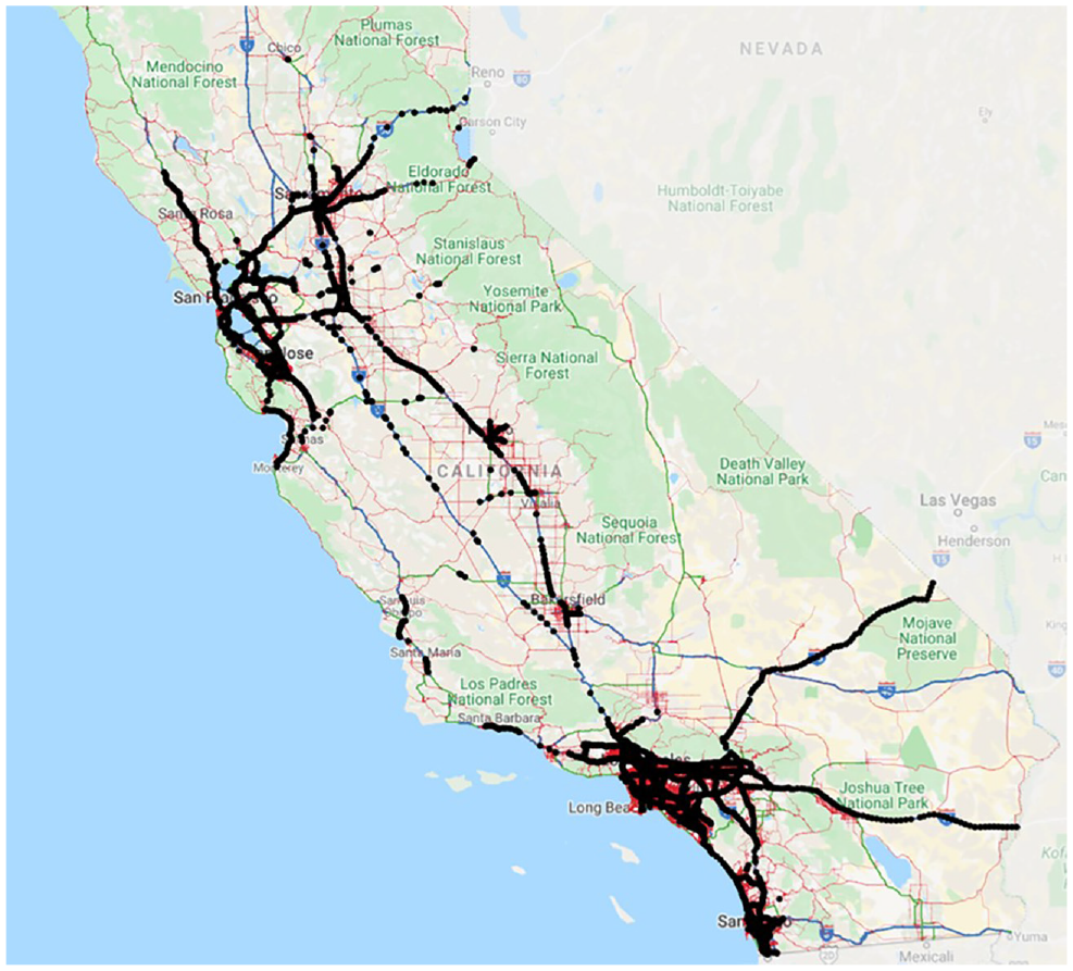
Locations of the traffic sensors in the road network of California.

Here the interchange selection procedure and cleaning of the raw data are explained. The movement speed of vehicles in a segment is an appropriate indicator of the traffic conditions, and many agencies are utilizing this data to monitor and operate their traffic networks. As traffic volumes enter a road at an intersection, they can considerably change the segment’s speed. Thus, the information on speed profiles and how they vary with time can significantly benefit the estimation of the traffic volumes and traffic conditions at road segments. Here, speeds at different sections of an interchange reflect the highway’s traffic flow patterns and those of the lower-level road connected to the highway through this interchange. Figure 2 illustrates the approaches and speeds that are considered in the model. Note that the off-ramp setting in this figure is the most common among the study off-ramps in this study, however, the types of off-ramp are not limited to the one illustrated.

In this interchange, “Ramp-1” is the ramp that is under consideration. The speeds that will be considered in the model are as follows:

- S_RT-D, FFS_RT-D: downstream speed and FFS of the exiting vehicles that are making a right turn.

- S_LT-U, FFS_LT-U: upstream speed and FFS of the exiting vehicles that are making a left turn.

- S_LT-D, FFS_LT-D: downstream speed and FFS of the exiting vehicles that are making a left turn.

- S_RT-U, FFS_RT-U: upstream speed, and FFS of the exiting vehicles that are making a right turn.

Figure 2.

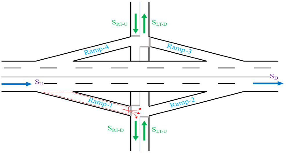
Schematic illustration of the considered speed profiles.

Although the number of installed count stations in California’s road network is extensive, not all of them record counts accurately. In addition, the speed profiles for all segments of interest are not available. Thus, before feeding the input to the model, a sanity check is required. This study defines four steps for validating the selected interchanges as follows:

Installation of three traffic count sensors: The interchange should have traffic count sensors installed on the off-ramp as well as upstream and downstream of the off-ramp, as shown in Figure 3.

Defined six unique TMC segments: Designation of specific TMC segments for the upstream and downstream of the off-ramp and the road connected to the freeway. In Figure 3, the yellow lines illustrate the unique TMC segments that must exist for the interchange, allowing extraction of movement speed at each time interval for each segment.

Conservation of flow: Volume counts on the three detectors should conform with an assumed maximum allowable deviation of %5, according to Equation 1.

V_{Upstream} = V_{Downstream} + V_{Ramp} + ϵ, | ϵ | \leq 0.05 V_{Upstream}

(1)

This equation must hold with $ϵ = 0$ if the vehicle detection is perfect. However, there are errors in vehicle detection in real-world situations, which causes the equation to hold with $| ϵ | > 0$ . The threshold that is considered in the paper is ${| ϵ |}_{m a x} = 5 %$ .

A minimum number of observations: The interchange should have an appropriate number of observations in the dataset to avoid bias in the dataset resulting in unreliable traffic count estimates. Based on the authors’ experiments in capturing ramp traffic flow variations, it was found that at least one month’s worth of data in an entire year (1 × 30 × 24 = 720) is an appropriate minimum number of records for each interchange.

Figure 3.

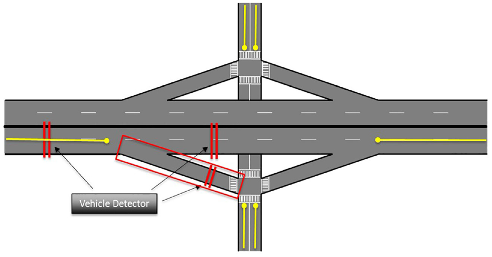
Schematic illustration of criteria for interchange selection as model input.

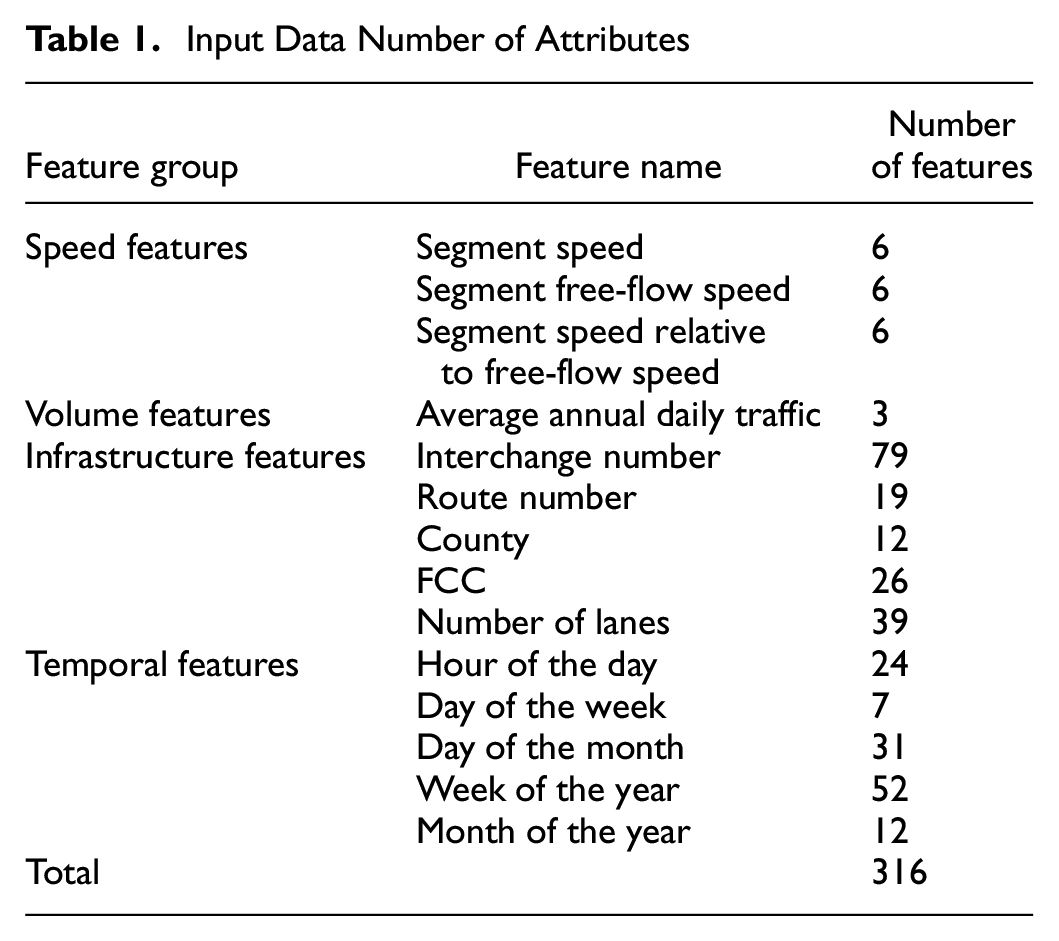
After cleaning the data, 79 interchanges with a total of 236,552 record rows are obtained as illustrated in Figure 4 with 316 features, as provided in Table 1 with details. Figure 5 shows the distribution of the off-ramp hourly counts. It can be seen in this figure that the distribution of flow counts covers a vast range of volumes, thus making the estimation harder. Also, the highest number of counts is located around 450 vehicles in an hour, and more than 90% of the observations have an off-ramp hourly count of less than 1,000 and more than 100 cars per hour.

Figure 4.

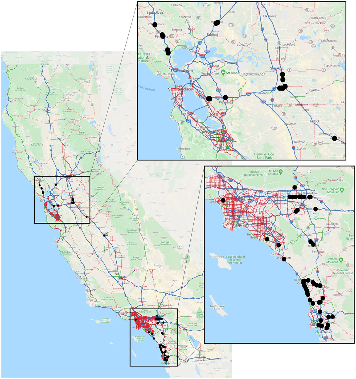
Locations of the 79 obtained interchanges.

Table 1.

Input Data Number of Attributes

Feature group	Feature name	Number of features
Speed features	Segment speed	6
	Segment free-flow speed	6
	Segment speed relative to free-flow speed	6
Volume features	Average annual daily traffic	3
Infrastructure features	Interchange number	79
	Route number	19
	County	12
	FCC	26
	Number of lanes	39
Temporal features	Hour of the day	24
	Day of the week	7
	Day of the month	31
	Week of the year	52
	Month of the year	12
Total		316

Figure 5.

Distribution of off-ramp hourly vehicle counts.

To illustrate how the data is distributed temporally, Figure 6 demonstrates the number of observations for each month, week, day, and hour. According to these radar charts, except for the hour of the day, the observations are relatively uniformly distributed. The distribution of observations in different hours of a day illustrates a skewness toward the morning and evening peak periods and morning off-peak hours, which will not negatively affect this study’s analysis as these hours are the most critical intervals from the perspective of operators and planners. Another crucial factor in the distribution of input data is the number of observations per interchange. A summary of this measure is as follows:

The average number of observations for each interchange: 2,994 observations

The median number of observations for each interchange: 2,650 observations

The standard deviation of observations for each interchange: 1,420 observations

Minimum number of observations for an interchange: 911 observations

Maximum number of observations for an interchange: 6,584 observations

Maximum possible number of observations for an interchange: 365×24=8,760 observations

Figure 6.

Distribution of the total observations for: (a) each month of the year, (b) each week of the year, (c) each day of the week, and (d) each hour of the day.

Thus, on average, 34% (= $\frac{2994}{8760})$ of the total possible observations for an interchange are available for this study. This sparsely distributed data makes it even harder for the modeler to train an accurate and robust model and will be discussed later.

Methodology

This study explores modeling the exiting flow counts from a freeway in an hour. The model selected for this study is a fully connected feedforward multi-layer neural network. As a deep learning model class, neural networks have great potential in data analysis and forecasting because they use distributed and hierarchical feature representation ( 37 ). Especially in the case of traffic volume estimation, previous studies ( 23 ) have shown the superiority of the fully connected feedforward multi-layer neural network relative to other models. Additionally, several studies have illustrated the superiority of deep learning models compared with other statistical models as the number of observations in the input data increases ( 23 , 38 , 39 ). A neural network model consists of neurons stacked in several layers. The first one is the input features, the last one represents the model prediction, and the middle ones are hidden layers of the model. The structure of these feed-forward fully connected models is in a manner that each neuron is connected to all the neurons in its previous layer. Typically, two issues arise during the training and testing of these models. The first problem is overfitting the model to the training set, in which the model learns the patterns in the training set. However, it cannot produce reliable estimates on other datasets. The overfitting problem is most often observed in models with too many parameters; however, there are common approaches for tackling it, such as L1 and L2 regularizations, and the addition of dropout layers. Generally, regularization methods tend to reduce overfitting by penalizing excess estimated weights by incorporating them in the loss function ( 40 ). In each training step, randomly selected neurons are temporarily ignored in the addition of the dropout technique, and weight updates are not applied to the neuron in the backward pass ( 41 ). In this study L2 regularization and the addition of dropout layers are employed to address the overfitting of the neural network models.

The second issue in deep learning models is computational efficiency during the training procedure. While the most popular activation function for shallow networks is the sigmoid function, this function is too slow for deep networks because it has a derivative between −0.25 and 0.25 ( 23 ). Thus, to increase the efficiency in the backpropagation process, the rectified linear unit (ReLU) function, a more efficient function ( 42 ), is used as the activation function with the following equation:

f (x) = \max (0, x)

(2)

In this study, several neural network models are trained with four hidden layers, each layer with 256 neurons to estimate off-ramps’ hourly flow. For each model, the training set is randomly drawn 25 times and is tested on the rest of the data. This procedure ensures capturing the effects of data variations on model estimates. The input variables are normalized to reduce the variations and adjust the scales ( 43 ), and the batch normalization technique is used to adjust the scales of neurons ( 44 ). As L2 regularization is not sufficient for tackling the overfitting issue in deep neural networks ( 23 ), random dropout layers are also added. The algorithm employed for training the models is the adaptive moment estimation (Adam) algorithm ( 45 ), a well-known stochastic gradient-based optimization method capable of handling high-dimensional parameter spaces in non-convex optimization problems.

The neural network model structure in Figure 7 illustrates the input variables, four hidden layers, each with 256 neurons, dropout layers, and the activation functions. The loss function of the neural network models is assumed to be the average of the squared errors between observed and estimated turning movement counts plus the regularization term, according to the formulation in Equation 3.

\begin{matrix} Loss = \frac{1}{n} \sum_{i = 1}^{n} {({\hat{y}}_{i} - y_{i})}^{2} \\ + \frac{λ}{2 n} \sum_{l = 1}^{L} \sum_{i = 1}^{n^{[l - 1]}} \sum_{j = 1}^{n^{[l]}} {(w_{ij}^{[l]})}^{2} \end{matrix}

(3)

where n is the number of observations; ${\hat{y}}_{i}$ is the estimated hourly turning movement count for observation i; $y_{i}$ is the observed hourly turning movement count for observation i; $λ$ is the regularization parameter; $w_{ij}^{[l]}$ is the weight factor associated with neuron j in layer l from neuron i in layer l-1.

The performance measures considered for evaluating the models are as follows:

Mean squared error (MSE): a measure for quality of estimates with a higher penalty for higher errors.

MSE = \frac{1}{n} \sum_{i = 1}^{n} {({\hat{y}}_{i} - y_{i})}^{2}

(4)

Mean absolute percentage error (MAPE): a measure that represents the relative accuracy of the model estimates.

MAPE = (\frac{1}{n} \sum_{i = 1}^{n} | \frac{{\hat{y}}_{i} - y_{i}}{y_{i}} |) * 100

(5)

Coefficient of determination (R²): a measure indicating the proportion of traffic volume variance explained by the model.

R^{2} = 1 - \frac{\sum_{i = 1}^{n} {(y_{i} - {\hat{y}}_{i})}^{2}}{\sum_{i = 1}^{n} {(y_{i} - \bar{y})}^{2}}

(6)

where $\bar{y}$ is the average of turning movement counts in an hour of all observations, and other parameters are introduced earlier.

Figure 7.

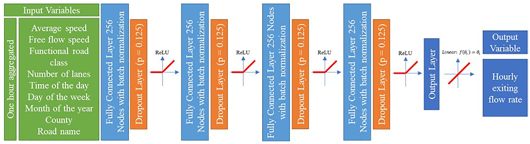
Structure of the neural network models.

Typically, the installation of traffic count sensors by the State Highway Administration (SHA) and state Department of Transportation authorities is a combination of permanently and temporarily installed detectors. The permanently installed detectors continuously collect data for a long duration (e.g., more than a month). In contrast, temporarily installed sensors collect data over a much shorter period and afterward are relocated at another site. This study analyzes the exiting flow counts from the two distinct perspectives of feature space evaluations and detector installation strategies. The benefits of inputting the segments and traffic flow characteristics of the lower-level road connected to the freeway are explored in the former perspective. The latter evaluates the estimation performance of the models according to the sensor installation strategy.

Analysis and Results

Explainability of Connected Lower-Level Road Inputs

A road network can be considered as a connected graph in which the links and vehicle movements in the links interact. In the context of exit flow from a freeway, the traffic flow conditions of the lower-level road connected to the freeway can play an important role. Therefore, feeding the features of these roads to the ramp flow estimation model is intuitively interpretable. However, to evaluate the explainability of these features, two separate models are trained and compared in this study ( 22 ). In the first, the “base model,” the lower-level road characteristics are not incorporated into the model. Thus, the model considers the attributes presented in Figure 7 solely for the upstream and downstream segments of the freeway. The results of training and testing this model are presented in Table 2. The second, the “all-inclusive model,” incorporates the base model features in addition to the attributes in Figure 7 for each one of the following segments of the lower-level road:

right-turn upstream,

right-turn downstream,

left-turn upstream, and

left-turn downstream.

To contend with the previously described detector installation scheme, the selection of data for training the exiting flow count models is as follows:

permanent vehicle detector installation for nine interchanges resulting in one year of data for each one,

temporary sensor installation for 70 interchanges yielding one week of data for each one.

Table 2.

Summary Statistics of the Results of the Base Model

Measure	Average	Standard deviation	Median	Minimum	Maximum
Training MSE	5,585	503	5,282	5,140	6,233
Validation MSE	23,944	2,922	23,413	19,884	28,209
Training MAPE	25.41	2.74	24.29	16.4	35.4
Validation MAPE	32.19	3.72	33.6	23.71	38.32
Training R²	0.847	0.03	0.855	0.752	0.929
Validation R²	0.734	0.05	0.757	0.578	0.856
Training set size	25,646	794	25,982	23,713	26,606
Runtime (seconds)	1,487	210	1,523	1,218	1,693

Note: MSE = mean squared error; MAPE = mean absolute percentage error.

The summary statistics of this model are presented in Table 3. Note that each model is trained and tested using k-fold cross-validation with k = 25. In comparing the performance measures of these models, it can be seen that the all-inclusive model has reduced the average validation MAPE by almost 9%, from 32% to 23%. The average validation R² has risen from 0.73 to 0.89. Additionally, with regard to variations in performance measures, it is observed that the all-inclusive model is more stable, thus providing more reliable estimations.

Table 3.

Summary Statistics of the Results of the All-Inclusive Model

	Average	Standard deviation	Median	Minimum	Maximum
Training MSE	4,739	906	4,654	3,788	6,236
Validation MSE	19,054	1,866	18,555	16,298	22,136
Training MAPE	17.29	1.25	16.2	12.19	22.91
Validation MAPE	22.93	2.32	22.13	15.48	30.56
Training R²	0.919	0.01	0.923	0.846	0.969
Validation R²	0.888	0.022	0.895	0.838	0.923
Training set size	26,284	360	26,438	25,523	26,811
Runtime (seconds)	1984	228	1985	1820	2,064

Note: MSE = mean squared error; MAPE = mean absolute percentage error.

Detector Installation Strategies

The installation of detectors for the previous models is assumed to be a combination of permanently and temporarily installed sensors. However, to explore each installation scheme’s contribution to the model performance, two distinct models are trained and tested. In the first, the “permanent detector installation model,” it is assumed that the vehicle detectors are permanently installed on several interchanges; thus, the ground truth data for these interchanges are available for the entire year. This strategy aims to estimate the hourly exiting flow counts at interchanges without installed detectors in the whole hours of a year. In the second, the “temporary detector installation model,” the sensors are installed for a short time interval at several interchanges. Thus, ground truth data for these interchanges are available for a short duration (e.g., with a maximum of one week). The goal here is to estimate hourly exiting flow counts at these interchanges during the hours of the year when detectors were not installed. The training and testing sets are drawn randomly 25 times accordingly to conform to each strategy.

Permanent Detector Installation Model

In the strategy of installing sensors permanently, the model is trained on the data of the interchanges with vehicle detectors. Further, the proportions of turning movements at other interchanges are estimated to evaluate the model’s accuracy. In this method, each random draw’s training set is obtained by dividing the data into two sets, for training and testing, according to interchange IDs; thus, resulting in two distinct sets of interchanges. For each random draw, 70 interchanges are selected (equivalent to almost 90% of all data interchanges) for model training, and the rest is utilized for testing the model. The results of training and validating the model for 25 training and validation sets drawn randomly from the whole dataset are shown in Table 4. According to the results shown in the table, the average error percentage of the model over the validation set is 50% and has relatively high variations, thus illustrating that the model estimates are unstable. This finding is further repeated based on the R², which has a negative minimum showing that on some validation sets, the model is performing worse than the reported average off-ramp flow. This model’s low performance is an interesting finding considering that the number of input data to the model is more than nine times that of previous models. Thus, one might reasonably deduce that the permanent detector installation’s contribution to the all-inclusive model is almost negligible.

Table 4.

Summary Statistics of the Results of the Permanent Detector Installation Model

	Average	Standard deviation	Median	Minimum	Maximum
Training MSE	21,296	1,639	20,134	17,479	25,383
Validation MSE	30,277	2,252	29,768	26,180	35,862
Training MAPE	45.38	2.43	46.34	41.24	48.94
Validation MAPE	51.45	19.48	50.09	25.22	78.98
Training R²	0.517	0.043	0.509	0.411	0.627
Validation R²	0.417	0.250	0.433	−0.344	0.575
Training set size	213,119	2,922	214,372	206,950	217,392
Runtime (seconds)	2,211	148	1,013	2,107	2,395

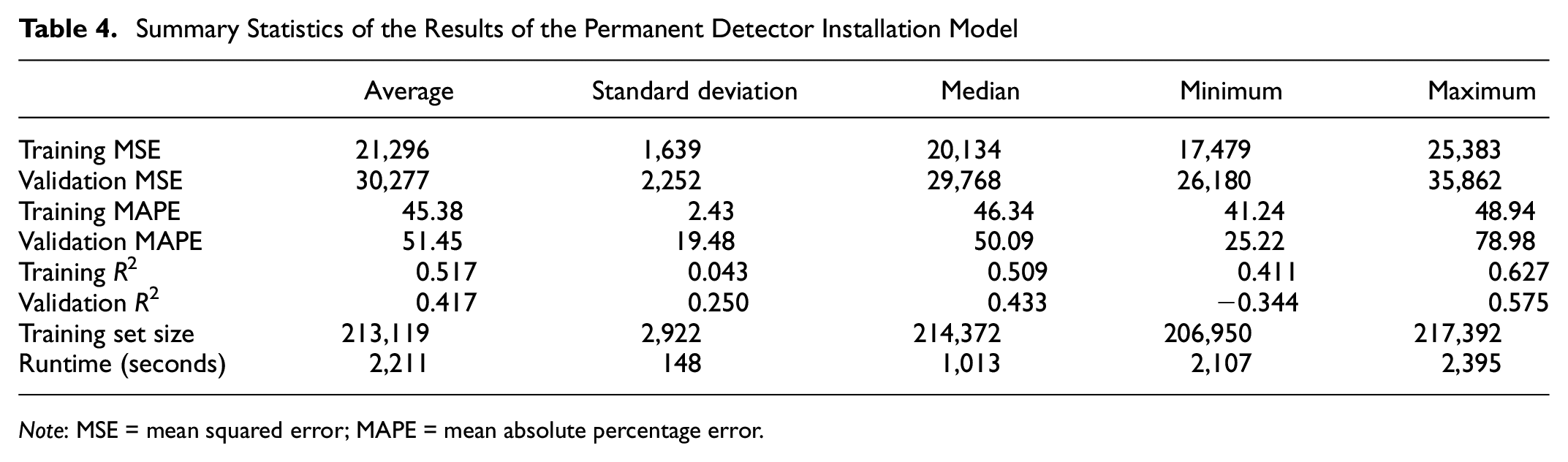
Note: MSE = mean squared error; MAPE = mean absolute percentage error.

Temporary Detector Installation Model

In this method, for each interchange, one and only one week is selected from the whole dataset and is added to the training dataset. Randomly selecting a week for each interchange in the real world is equivalent to temporarily installing sensors for a single week on each interchange. As described above, the average number of observations in a week for each interchange in the dataset is almost 34% of the maximum possible observations in a week because of the low-quality data collection procedure. This model is trained with 25 different random training validation sets. The model performance summary is presented in Table 5. According to the results in the table, this model is relatively stable; however, it is weaker than the all-inclusive model. For instance, the average validation MAPE has increased from 23% to 29%, and the average validation R² has reduced from 0.89 to 0.76. Interestingly, for the total number of 79 interchanges, the average number of observations used for training the model is 3,253, which means that on average, for each interchange, less than 42 h worth of data ( $= \frac{3253}{79}$ ) is employed for training the model. Thus, installing sensors on interchanges for two days and nights enables training a model that can estimate the exiting flow counts with an average of 30% error for the entire year.

Table 5.

Summary Statistics of the Results of the Temporary Detector Installation Model

	Average	Standard deviation	Median	Minimum	Maximum
Training MSE	5,438	833	5,535	5,039	5,742
Validation MSE	21,756	2,319	22,173	17,625	25,451
Training MAPE	21.34	3.99	19.75	13.01	29.9
Validation MAPE	29.12	4.14	35.92	19.44	38.09
Training R²	0.943	0.021	0.948	0.866	0.969
Validation R²	0.763	0.115	0.788	0.578	0.916
Training set size	3,253	212	3,253	2,770	3,697
Runtime (seconds)	2,758	1,152	2,457	1,227	4,643

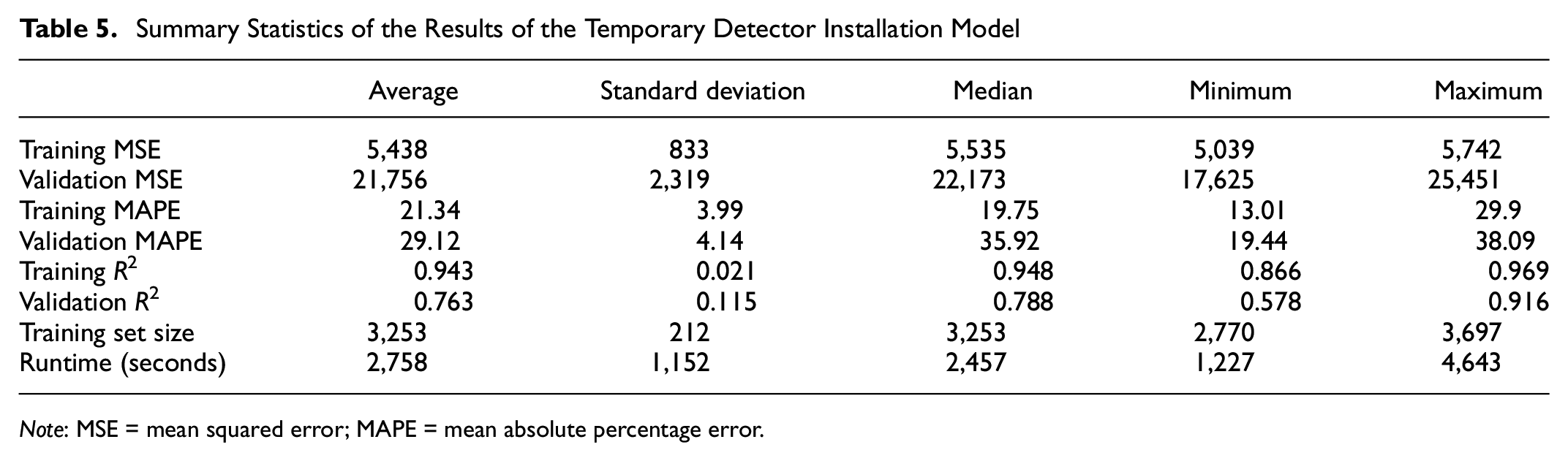
Note: MSE = mean squared error; MAPE = mean absolute percentage error.

Summary and Conclusion

Freeways are a significant determinant of the road network traffic conditions considering that a large volume of vehicles traverse them. The interaction between freeways and the rest of the network is through on- and off-ramps. An accurate estimation of the ramps’ traffic volume can benefit the system operators in reducing traffic congestion, thus increasing mobility. This study estimates the hourly off-ramp traffic volume using a fully connected feedforward multi-layer neural network. The proposed neural network model has four fully connected hidden layers, each layer consisting of 256 neurons with the assumption of the ReLU activation function. To address the overfitting and computational efficiency of the model, L2 regularization, batch normalization, and the addition of dropout layers are performed.

The data source for ramp traffic volume is the PeMS website, a repository for volume count records, among other traffic flow measures of California’s road network. After cleaning the data, observations from 79 interchanges remain with 236,552 records for the year 2019. The average number of observations for each interchange in the dataset is 2,994, indicating the data’s sparsity and low-quality data collection. All models are trained and tested 25 times with random data splits to account for the dataset variations and enable a more robust generalization of the findings.

In the first step, the impacts of inputting the connected lower-level road features and their traffic flow characteristics on the model’s performance were explored. Thus, two models are trained and tested; the first, the “base model,” without the mentioned attributes, and the second, the “all-inclusive model,” with the inclusion of those attributes. As the detector installation in real-world situations is a combination of permanent and temporarily installed detectors, a combined detector installation is assumed for each of these models. Nine randomly selected interchanges are considered to have permanent detectors installed; thus, their entire year’s data is added to the training set. For the rest of the 70 interchanges, only the data collected during a single week is incorporated into the training set. The base model had an average validation MAPE of 32%, while the same measure for the all-inclusive model was obtained as 23%. The average validation R² of the former model was 0.73, while the latter was 0.89. Additionally, with regard to the model performance’s stability, the all-inclusive model is more stable than the base model in both measures. Therefore, it is concluded that a significant gain in the flow estimation model’s performance is achieved by incorporating the input features of the connected lower-level roads.

In the second step of the analysis, the contribution of each detector installation strategy (e.g., permanent or temporary) to the all-inclusive model is examined. In the permanent installation model, yearly data of 70 randomly selected interchanges are used for training. The results of hourly off-ramp flow estimation of this model on the nine remaining interchanges illustrated a weak performance for this model—a minimum validation R² of negative is reported. This model’s poor performance can be attributed to the fact that the model cannot construct the dependencies and correlations between ramp traffic volumes at different interchanges. The temporary installation model yields an acceptable performance considering that the model uses the data of less than 42 h for each interchange on average. Thus, it is concluded that the model can capture and establish the relations between the volume counts and the temporal attributes.

This study sheds more light on an area that has not received much attention in previous studies. The findings help researchers gain more insight into the traffic volume estimation of off-ramps with regard to the required data and the modeling framework. This study also provides valuable information for the transportation system operators about the appropriate traffic sensor installation strategies, yielding a more accurate traffic volume estimation model. Another contribution of the current research is to ramp metering applications, where having a traffic volume estimation is priceless. As a part of future work, the introduced methodology will be expanded to consider both on- and off-ramps to establish a more general framework for ramp traffic volume estimation. Further, to address the detrimental impacts of the road network structure absence in the proposed methodology, more advanced models capable of embedding this structure and building the relations between link traffic flow characteristics will be employed in future studies. Finally, the methodology of the current study will be developed to address traffic flow prediction as well.

Footnotes

Author Contributions

The authors confirm contribution to the paper as follows: study conception and design: AN, SZ, AH; data collection: AN; analysis and interpretation of results: AN, SZ, AH; draft manuscript preparation: AN, SZ. All authors reviewed the results and approved the final version of the manuscript.

Declaration of Conflicting Interests

The author(s) declared no potential conflicts of interest with respect to the research, authorship, and/or publication of this article.

Funding

The author(s) received no financial support for the research, authorship, and/or publication of this article.

ORCID iDs

Amir Nohekhan

Sara Zahedian

Ali Haghani

References

Cascetta

Transportation Systems Analysis: Models and Applications. Springer Science & Business Media, Boston, MA, 2009.

Bera

Rao

K. V.

Estimation of Origin-Destination Matrix from Traffic Counts: The State of the Art. European Transport, Vol. 49, 2011, pp. 3–23.

Maher

M. J.

Inferences on Trip Matrices from Observations on Link Volumes: A Bayesian Statistical Approach. Transportation Research Part B: Methodological, Vol. 17, No. 6, 1983, pp. 435–447.

Cascetta

Inaudi

Marquis

Dynamic Estimators of Origin-Destination Matrices Using Traffic Counts. Transportation Science, Vol. 27, No. 4, 1993, pp. 363–373.

Zhou

Mahmassani

H. S.

Dynamic Origin-Destination Demand Estimation Using Automatic Vehicle Identification Data. IEEE Transactions on Intelligent Transportation Systems, Vol. 7, No. 1, 2006, pp. 105–114.

De Villa

A. R.

Casas

Breen

Perarnau

Minimising GEH in Static OD Estimation. In Proc., Australasian Transport Research Forum, Brisbane, Australia, Vol. 4, 2013.

Marzano

Papola

Simonelli

Limits and Perspectives of Effective O–D Matrix Correction Using Traffic Counts. Transportation Research Part C: Emerging Technologies, Vol. 17, No. 2, 2009, pp. 120–132.

Peeta

Ziliaskopoulos

A. K.

Foundations of Dynamic Traffic Assignment: The Past, the Present and the Future. Networks and Spatial Economics, Vol. 1, No. 3, 2001, pp. 233–265.

Wang

Papageorgiou

Real-Time Freeway Traffic State Estimation Based on Extended Kalman Filter: A General Approach. Transportation Research Part B: Methodological, Vol. 39, No. 2, 2005, pp. 141–167.

10.

Guo

Ding

Chen

Freeway Traffic Speed Estimation of Mixed Traffic Using Data from Connected and Autonomous Vehicles with a Low Penetration Rate. Journal of Advanced Transportation, Vol. 2020, 2020, pp. 1–13.

11.

Chu

Recker

Adaptive Kalman Filter Based Freeway Travel Time Estimation. Presented at 84th Annual Meeting of the Transportation Research Board, Washington, D.C., 2005.

12.

Liu

Van Zuylen

Van Lint

Salomons

Predicting Urban Arterial Travel Time with State-Space Neural Networks and Kalman Filters. Transportation Research Record: Journal of the Transportation Research Board, 2006. 1968: 99–108.

13.

Xie

Zhang

Short-Term Traffic Volume Forecasting Using Kalman Filter with Discrete Wavelet Decomposition. Computer-Aided Civil and Infrastructure Engineering, Vol. 22, No. 5, 2007, pp. 326–334.

14.

Liu

Fan

Ding

An Innovative Information Fusion Method with Adaptive Kalman Filter for Integrated INS/GPS Navigation of Autonomous Vehicles. Mechanical Systems and Signal Processing, Vol. 100, 2018, pp. 605–616.

15.

Pakdamanian

Sheng

Baee

Heo

Kraus

Feng

DeepTake: Prediction of Driver Takeover Behavior Using Multimodal Data. arXiv Preprint arXiv:2012.15441, 2020.

16.

Zahedian

Sadabadi

K. F.

Nohekhan

Localization of Autonomous Vehicles: Proof of Concept for a Computer Vision Approach. In Proc., 2019 ITS America Annual Meeting, ITSWC, Washington, DC, 2019.

17.

Joerger

Hassani

A New Data Association Method Using Kalman Filter Innovation Vector Projections. In Proc., 2020 IEEE/ION Position, Location and Navigation Symposium (PLANS), Portland, OR, IEEE, 2020, pp. 318–327.

18.

Ebnali

Fathi

Lamb

Pourfalatoun

Motamedi

Using Augmented Holographic UIs to Communicate Automation Reliability in Partially Automated Driving. In AutomationXP @ CHI

19.

Mousavi

S. M.

Zhang

Parr

S. A.

Pande

Wolshon

Identifying High Crash Risk Highway Segments Using Jerk-Cluster Analysis. In Proc., International Conference on Transportation and Development 2019: Smarter and Safer Mobility and Cities, Alexandria, VA, American Society of Civil Engineers, Reston, VA, 2019, pp. 112–123

20.

Vanajakshi

Rilett

L. R.

A Comparison of the Performance of Artificial Neural Networks and Support Vector Machines for the Prediction of Traffic Speed. In Proc., IEEE Intelligent Vehicles Symposium, Parma, Italy, IEEE, 2004, pp. 194–199.

21.

Xia

Y. J.

Rao

Short-Term Traffic Flow Forecasting for Urban Roads Using Data-Driven Feature Selection Strategy and Bias-Corrected Random Forests. Transportation Research Record: Journal of the Transportation Research Board, 2017. 2645: 157–167.

22.

Zahedian

Sekuła

Nohekhan

Vander Laan

Estimating Hourly Traffic Volumes Using Artificial Neural Network with Additional Inputs from Automatic Traffic Recorders. Transportation Research Record: Journal of the Transportation Research Board, 2020. 2674: 272–282.

23.

Sekuła

Marković

Vander Laan

Sadabadi

K. F.

Estimating Historical Hourly Traffic Volumes via Machine Learning and Vehicle Probe Data: A Maryland Case Study. Transportation Research Part C: Emerging Technologies, Vol. 97, 2018, pp. 147–158.

24.

Parsa

A. B.

Taghipour

Derrible

Mohammadian

A. K.

Real-Time Accident Detection: Coping with Imbalanced Data. Accident Analysis & Prevention, Vol. 129, 2019, pp. 202–210.

25.

Mokhtarimousavi

Anderson

J. C.

Azizinamini

Hadi

Factors Affecting Injury Severity in Vehicle-Pedestrian Crashes: A Day-of-Week Analysis Using Random Parameter Ordered Response Models and Artificial Neural Networks. International Journal of Transportation Science and Technology, Vol. 9, No. 2, 2020, pp. 100–115.

26.

Esfahani

H. N.

Song

Christensen

A Deep Neural Network Approach for Pedestrian Trajectory Prediction Considering Heterogeneity. Presented at 99th Annual Meeting of the Transportation Research Board, Washington, D.C., 2020.

27.

Stone

Cross-Validatory Choice and Assessment of Statistical Predictions. Journal of the Royal Statistical Society: Series B (Methodological), Vol. 36, No. 2, 1974, pp. 111–133.

28.

Zahedian

Nohekhan

Sadabadi

K. F.

Dynamic Toll Prediction Using Historical Data on Toll Roads: Case Study of the I-66 Inner Beltway. arXiv Preprint arXiv:2104.10684, 2021.

29.

Kan

Wang

Sun

Shao

Papageorgiou

A Novel Approach to Estimating Missing Pairs of On/Off Ramp Flows. IEEE Transactions on Intelligent Transportation Systems, Vol. 22, No. 2, 2020, pp. 1287–1305.

30.

Schrank

Eisele

Lomax

Bak

Appendix A: Methodology for the 2015 Urban Mobility Scorecard. Technical Report. Texas Transportation Institute, Texas A&M University, 2015. http://tti.tamu.edu/documents/mobility-scorecard-2015-wappx.pdf.

31.

Liu

X. C.

Markovic

Phillips

Inferencing Hourly Traffic Volume Using Data-Driven Machine Learning and Graph Theory. Computers, Environment and Urban Systems, Vol. 85, 2021, p. 101548.

32.

Mashhadi

A. H.

Farhadmanesh

Rashidi

Marković

. Review of Methods for Estimating Construction Work Zone Capacity. Transportation Research Record: Journal of the Transportation Research Board, 2021. 03611981211002202.

33.

Caltrans, Performance Measurement System (PeMS), California Department of Transportation. 2019. http://pems.dot.ca.gov.

34.

The Regional Integrated Transportation Information System (RITIS). CATT Laboratory, University of Maryland, 2020. http://www.cattlab.umd.edu/?portfolio=ritis. Accessed January 14, 2020.

35.

Operations Performance Measurement Program. The Urban Congestion Report (UCR): Documentation and Definitions. FHWA, U.S. Department of Transportation. https://ops.fhwa.dot.gov/perf_measurement/ucr/documentation.htm. Accessed November 3, 2020.

36.

Updated Guidance for the Functional Classification of Highways. Federal Highway Administration. U.S. Department of Transportation, 2008. https://www.fhwa.dot.gov/policy/ohpi/hpms/fchguidance.cfm.

37.

Huang

Song

Hong

Xie

Deep Architecture for Traffic Flow Prediction: Deep Belief Networks with Multitask Learning. IEEE Transactions on Intelligent Transportation Systems, Vol. 15, No. 5, 2014, pp. 2191–2201.

38.

Najafabadi

M. M.

Villanustre

Khoshgoftaar

T. M.

Seliya

Wald

Muharemagic

Deep Learning Applications and Challenges in Big Data Analytics. Journal of Big Data, Vol. 2, No. 1, 2015, pp. 1–21.

39.

Taghipour

Parsa

A. B.

Mohammadian

A. K.

A Dynamic Approach to Predict Travel Time in Real Time Using Data Driven Techniques and Comprehensive Data Sources. Transportation Engineering, Vol. 2, 2020, p. 100025.

40.

A. Y.

Feature Selection, L₁ vs. L₂ Regularization, and Rotational Invariance. In Proc., Twenty-First International Conference on Machine Learning, Banff, Alberta, Canada, Association for Computing Machinery, New York, 2004, p. 78.

41.

Dahl

G. E.

Sainath

T. N.

Hinton

G. E.

Improving Deep Neural Networks for LVCSR Using Rectified Linear Units and Dropout. In Proc., 2013 IEEE International Conference on Acoustics, Speech and Signal Processing, Vancouver, British Columbia, Canada, IEEE, 2013, pp. 8609–8613.

42.

Krizhevsky

Sutskever

Hinton

G. E.

ImageNet Classification with Deep Convolutional Neural Networks. Communications of the ACM, Vol. 60, No. 6, 2017, pp. 84–90.

43.

Bishop

C. M.

Neural Networks for Pattern Recognition. Oxford University Press, Oxford, 1995.

44.

Ioffe

Szegedy

Batch Normalization: Accelerating Deep Network Training by Reducing Internal Covariate Shift. In Proc., International Conference on Machine Learning, Lille, France, PMLR, Vol. 37, 2015, pp. 448–456.

45.

Kingma

D. P.

Adam: A Method for Stochastic Optimization. arXiv Preprint arXiv:1412.6980, 2014.