Pavement Fatigue Damage Simulations Using Second-Generation Mechanistic-Empirical Approaches

Abstract

This article aims to demonstrate the advanced features of two second-generation mechanistic-empirical (ME) pavement analysis engines by focusing on their ability to conduct fatigue performance analysis. First, a comprehensive review is presented of both mechanistic and empirical damage models, underlining the additional features of CalME and FlexPAVE™ over AASHTOWare Pavement ME Design. Then, the capabilities of these methodologies are demonstrated by simulating the fatigue damage performance of an example study section. For these simulations the mechanical properties of four asphalt concrete mixtures, assembled in the laboratory with similar mix design attributes but diverse fatigue characteristics, were utilized. The empirical transfer functions were initially calibrated against field cracking for the unmodified mixture cracking predictions. After that, fatigue damage simulations for the other three mixtures were performed. The results showed a similar ranking in fatigue cracking performance for both software simulations. Polymer-modified mixtures exhibited higher fatigue cracking resistance, whereas the unmodified mixture showed the worst cracking resistance. However, significant differences in cracking initiation and progression rates were observed for all mixture simulations before and after calibration. This discrepancy was related to the different approaches to considering traffic loads in each software system, single axle in FlexPAVE™ and axle spectrum in CalME. Finally, current, and future enhancements for both analysis engines are briefly discussed.

Pavement structures are complex systems that involve the interaction of diverse variables, including material characteristics, traffic loading, environmental conditions, aging, and distress evolution, and such variables are changing continuously throughout its service life. For this reason, the procedures used to design these structures should be updated periodically, improving their capability to simulate pavement service conditions. The empirically based AASHTO method can be used as an example of historical pavement design evolution. This method initially emerged primarily from analysis of the AASHO test road but was also informed by other test sites and the prevailing engineering knowledge at the time. The original performance function that became the design equation was released in 1966, but the first broadly applicable version did not appear until 1972. This equation was subsequently enhanced throughout the years to cover a broader range of designs, incorporating overlay and rehabilitation design procedures, reliability, resilient modulus for soil support, and improved consideration of environmental conditions and traffic data, to name a few ( 1 ).

Despite these enhancements, limitations with this basic approach have appeared and currently many agencies have adopted, or are moving toward adoption of, mechanistic-empirical (ME) approaches. ME methodologies use a mathematical model to calculate the pavement response in terms of stress, strain, or displacement under loading and prevailing environmental conditions, constituting the mechanical part of the process. Such responses are then related to the performance of the pavement through transfer functions to determine the distress modes, comprising the empirical part ( 2 ).

The idea of using mechanics as a basis for pavement design was contemporary with the thinking that resulted in the empirical design methods. However, many roadblocks existed including computational time and the simplifying assumptions that the computational times necessitated. In addition, the need was identified, in the end, to include empirical calibration factors to link mechanistic response to measurable distresses. This is why contributions of the AASHO test road to pavement design are closely related to the development of what are called “analytic based design procedures” ( 3 ), in addition to the empirical design method that was the initial product. These analytical methods calculate permissible values at critical locations in a pavement structure using a mechanistic approach, but they have the limitation that most of them were calibrated empirically to accommodate climatic factors, construction practices, and the materials employed, using data from a single location and limited field conditions ( 4 ).

For this reason, in the authors’ opinion, the first complete ME pavement design methodology was developed under NCHRP 1-37A Project, Guide for the Design of New and Rehabilitated Pavement Structures, because it incorporates additional features such as climate impacts, comprehensive material properties characterization, and axle load spectra characterization of traffic for predicting diverse pavement distresses over the designated period. Then, in 2008 the Mechanistic-Empirical Pavement Design Guide Manual of Practice (MEPDG) was released, documenting the design methodology calibrated using in-service pavement performance data. Eventually, in 2011, AASHTO released the AASHTOWare Pavement ME Design™ (hereafter “Pavement ME”) software that expands and improves the features of the computational software developed as a part of NCHRP 1-37A Project ( 5 ).

Pavement ME represents a paradigm shift in pavement design practices since it provides a more realistic characterization of in-service pavements and provides uniform guidelines for designing the in-common features of flexible, rigid, and composite pavements ( 6 ). For this reason, similar to the empirical AASHTO guide, Pavement ME has changed pavement practice, and several road agencies around the world are working in its local calibration and implementation ( 7 , 8 ). However, Pavement ME requires over 100 inputs to accomplish the pavement performance simulations over the design life, involving significant time and cost to implement it. Consequently, for this and other reasons, several ME-based approaches, such as CalME ( 9 ) and FlexPAVE™ ( 10 ), were developed after Pavement ME was released, with additional features or improvements to tackle certain shortcomings. To distinguish these approaches from Pavement ME, these analysis engines are referred to here as the second-generation approaches, since they are not design-centric methodologies and can be applicable to other activities such as performance engineering specifications, quality assurance, or management.

This study presents a comprehensive overview of the asphalt concrete (AC) undamaged and damaged models, and the empirical transfer functions, highlighting the additional features in CalME version 2.0, developed by the University of California Pavement Research Center, and FlexPAVE™ version 1.1, developed by North Carolina State University, over Pavement ME, focusing on fatigue cracking performance. Then, the capability of these features is demonstrated by simulating the observed pavement fatigue performance for a study section, using four AC mixtures, assembled in the laboratory, to simulate their cracking resistance under the same load traffic, temperature, and pavement structure conditions.

Background

Pavement ME

The Pavement ME methodology uses an incremental damage approach based on the accumulation of damage using Miner’s hypothesis as a function of time and traffic to estimate the distress for each analysis interval in a pavement structure. The structural layers and foundation are subdivided into sublayers for the computation of the critical pavement responses in each sublayer via the multilayer linear elastic analysis (MLEA) program JULEA (Jacob Uzan Layered Elastic Analysis) ( 5 ). Similarly, pavement layer modulus values are adjusted with time, temperature, and moisture conditions predicted on an hourly basis by the Enhanced Integrated Climatic Model (EICM). However, for AC layers, the temperature in each sublayer is combined into five successive groups or quintiles of the calculated values in each month of analysis for load-related distress prediction. Then, the average temperature within each quintile of a sublayer for each month is used to determine the dynamic modulus (|E*|) of that sublayer, assuming equal truck traffic distribution for that month ( 11 ).

The calculated |E*| is used to compute the horizontal strains at the critical depths on a horizontal grid to determine the location of the maximum fatigue damage in the AC layers and to compute the vertical strains throughout the depth to predict rutting in all layers. The general form of the |E*| master curve is the sigmoidal function, and it can be represented, as shown in Equation 1, in accordance with AASHTO R62 ( 12 ). The reduced frequency is computed using the time–temperature superposition (t-TS) principle, and shift factors are related to the viscosity of the asphalt binder via Equation 2. For unaged conditions, the viscosity of the asphalt binder at the temperature of interest is determined from the ASTM viscosity–temperature relationship ( 13 ) defined by Equation 3.

\log (| E^{*} |) = δ + \frac{α}{1 + e^{β + γ \log (f_{r})}}

(1)

\log (f_{r}) = \log (f) + c [\log (η) - \log (η_{T_{R}})]

(2)

\log (η) = 10^{[A + VTS \log (T)]}

(3)

where

$α, β, δ, and γ$ are fitting parameters;

f_r is the reduced frequency in Hz;

f is the loading frequency at the test temperature in Hz;

c is a fitting coefficient;

η is the viscosity of the binder at the test temperature in cP (centipoise);

T_R is the reference temperature in °R (Rankine);

$η_{T_{R}}$ is the viscosity of the binder at the reference temperature in cP;

A and VTS are the parameters of the binder viscosity–temperature susceptibility relationship; and

T is the test temperature in °R.

Only the bottom-up fatigue cracking (alligator cracking) is described here since it is of primary interest to the aim of this article and is often the critical distress for structural design. The Pavement ME assumes that the alligator cracks initiate at the bottom of the AC layers and propagate to the surface with continued trafficking. The shift function to predict the allowable number of axle-load applications which is needed for the incremental damage index approach to predict both types of load-related cracks is given by Equation 4.

N_{f - AC} = K_{f 1} (C) (C_{H}) B_{f 1} {(ε_{t})}^{K_{f 2} B_{f 2}} {(E_{AC})}^{K_{f 3} B_{f 3}}

(4)

C = 10^{M}

(5)

M = 4.84 (\frac{V_{be}}{V_{a} + V_{be}} - 0.69)

(6)

C_{H} = \frac{1}{0.000398 + \frac{0.003602}{1 + e^{(11.02 - 3.49 H_{AC})}}}

(7)

where

$N_{f - AC}$ is the allowable number of axle-load applications for flexible pavement;

$ε_{t}$ is the tensile strain at critical locations, calculated by the structural response model, in./in.

$E_{AC}$ is the dynamic modulus of the AC measured in compression, in psi (pounds per square inch);

$K_{f 1}, K_{f 2}, K_{f 3}$ are the global calibration coefficients;

$B_{f 1}, B_{f 2}, B_{f 3}$ are the local field calibration constants;

$V_{be}$ is the effective asphalt content by volume;

$V_{a}$ is the percentage of air voids in the AC mixture;

$C_{H}$ is the thickness correction term for alligator cracking; and

$H_{AC}$ is the total AC thickness, in inches.

Subsequently, Pavement ME calculates the incremental damage indices on a horizontal grid pattern throughout the AC layers at critical depths. The incremental damage index (ΔDI) is calculated by dividing the actual number of axle loads by the allowable number of axle loads within a specific time increment and axle-load interval for each type of axle. The cumulative damage index at the bottom of the AC layers (DI_Bottom) for each critical location is determined by summing the incremental damage indices over time (Equation 8). Finally, the area of alligator cracking is calculated from the total damage over time via transfer function given by Equation 9, which is the relationship used to predict the amount of alligator cracking on an area basis (FC_Bottom).

D I_{Bottom} = \sum {(Δ DI)}_{j, m, l, p, T} = \sum {(\frac{n}{N_{f - AC}})}_{j, m, l, p, T}

(8)

F C_{Bottom} = (\frac{1}{60}) (\frac{C_{4}}{1 + e^{(C_{1} C_{1}^{*} + C_{2} C_{2}^{*} Log (D I_{Bottom}))}})

(9)

C_{1}^{*} = - 2 C_{2}^{*}

(10)

C_{2}^{*} = - 2.40874 - 39.748 {(1 + H_{AC})}^{- 2.856}

(11)

where

n is the actual number of axle-load applications within a specific time period;

j is the axle-load interval;

m is the axle-load type (single tandem, tridem, or quad);

l is the truck type using the truck classification groups included in the Pavement ME;

p is the month;

T is the median temperature for the five temperature intervals or quintiles used to subdivide each month in °F or °C; and

C_1,2,4 are the transfer regression constants.

CalME 2.0

CalME uses an incremental-recursive (IR) pavement performance approach, where incremental refers to the performance prediction for each time increment. The default duration for this increment is 30 days, but it can be changed by the user. The term “recursive” refers to the damage condition update using the damage state or level predicted from the previous time increment before the incremental damage is calculated for the next increment ( 14 ). In this approach, material properties vary with damage in addition to temperature conditions during the design period. The computation of the damage is based on the structural response obtained through MLEA and damage accumulation ( 15 ).

For pavement temperature calculation, CalME uses the surface temperatures in a database generated by EICM for predefined climate zones in California. Then, it solves for pavement temperature profile by using 1-D finite element formulation with a finite difference step ( 16 ). One day is divided into periods, with a default of five periods with 5- and 4-h intervals, for each monthly time increment of the design period to represent the temperature and truck traffic distribution of the whole-time increment. Therefore, the AC stiffness is modeled as a function of temperature and loading time, also using the sigmoidal function (Equation 12). Similarly, the time–temperature shift factors are computed as a function of the viscosity to consider the effects of aging and healing using complementary models. Thus, the reduced time is a function of loading duration and temperature (Equation 13), and the loading time depends on the vehicle speed and layer thickness, assuming a uniform distribution of stress and tire contact area (Equation 14). Finally, binder viscosity can be calculated from the ASTM viscosity–temperature relationship ( 13 ) defined by Equation 15.

\log (| E^{*} |) = δ + \frac{α}{1 + ex p^{(β + γ \log (t_{r}))}}

(12)

t_{r} = l_{t} \times {(\frac{η}{η_{ref}})}^{a_{T}}

(13)

l_{t} = \frac{200 mm + 2 \times z_{1 / 3}}{v}

(14)

\log - \log η = A + VTS \cdot \log T

(15)

where

$α, β, δ, and γ$ are fitting parameters;

t_r is the reduced frequency in seconds;

l_t is the loading time in seconds;

η is the viscosity of the binder at the loading temperature in cP;

$η_{ref}$ is the viscosity of the binder at the reference temperature in cP;

a_T is the temperature shift factor;

$z_{1 / 3}$ is the depth of the AC layer at the upper 1/3 division point in mm;

v is the vehicle speed in mm/s;

A and VTS are the parameters of the binder viscosity–temperature susceptibility relationship; and

T is the test temperature in °K (Kelvin).

In CalME, the surface cracking density caused by fatigue is a function of the damage in the AC layers. The fatigue damage is accumulated at a rate that is determined by tensile strain caused by traffic loading and temperature variation. Thus, fatigue damage to the material stiffness is defined by Equation 16. For this purpose, the damage term (Equation 17) converts laboratory fatigue performance to the field fatigue performance, relating the number of truck traffic applications for each time increment and the shift function to predict the allowable number of axle-load applications (Equation 18) in an incremental power function. Therefore, for a specific AC, the material-dependent parameters, α_f, A, and β, are required to incorporate the laboratory fatigue properties, and the calibrated fatigue shift factor (FSF) is used to account for the difference between laboratory and field fatigue performance.

\log (| E^{*} |) = δ + \frac{α \times (1 - ω)}{1 + ex p^{(β + γ \log (t_{r}))}}

(16)

ω = {(\frac{MN}{FSF \times M N_{p}})}^{α_{f}}

(17)

M N_{p} = A \times {(\frac{ε}{ε_{ref}})}^{β} \times {(\frac{E}{E_{ref}})}^{\frac{β}{2}}

(18)

where

ω is the fatigue damage;

MN is the number of load applications in millions;

MN_p is the allowable number of load repetitions in millions;

ε is the bending strain at the bottom of the asphalt layer in με (microstrain);

ε_ref is the reference bending tensile; and

E_ref is the reference stiffness.

CalME assumes that the fatigue cracking initiates at the bottom of the AC layer and then propagates up to the surface as the simulation of pavement life progresses, that is, the bottom-up fatigue cracking process. For this purpose, the amount of cracking on the surface (when the cracking is visible), defined as crack initiation, must be assumed. Consequently, a value of 5% of initial cracking is established, based on pavement calibration studies ( 17 ). The correlation between AC damage and surface crack density is described by the empirical equation shown in Equation 19, and the damage to the surface layer at crack initiation is determined from Equation 20.

C = \frac{C_{\max} \times (ω_{initiation}^{α_{1}} - 1)}{ω_{initiation}^{α_{1}} - \frac{C_{\max}}{C_{i}} + (\frac{C_{\max}}{C_{i}} - 1) \times ω^{α_{1}}}

(19)

ω_{initiation} = \frac{1}{1 + {(\frac{h_{CA}}{h_{0}})}^{α_{2}}}

(20)

where

C is the surface crack density;

α₁ is a model parameter;

ω_initiation is the damage corresponding to crack initiation;

C_i is the surface crack density corresponding to crack initiation damage (ω_initiation), assumed to be 5% wheel path cracking;

C_max is the maximum surface crack density (100% wheel path cracking);

h_AC is the combined thickness of the AC layers; and

h₀ and α₂ are empirical model parameters.

FlexPAVE™ 1.1

FlexPAVE™ is a pavement response and performance analysis tool based on an efficient framework developed by combining time-scale separation and layered viscoelastic analysis ( 10 ). The basic computational framework uses time-scale differences among temperature variation, traffic frequency variations, and fatigue/rutting evolution to reduce the number of pavement response analyses. In addition, it uses a stress–strain analysis using a layered structural approach based on a Fourier finite element (FFE) transform, to capture the viscoelasticity effects of materials, temperature, and the moving nature of loads ( 18 ). Fatigue cracking and rutting pavement performance are predicted using mechanics-based models ( 19 ).

The temperature variation produces changes in stiffness and thermal stresses for AC materials in FlexPAVE™ ( 20 ). The temperature pavement profile on an hourly basis is divided into three analysis segments, assuming that each segment has a constant temperature and associated thermal stress/strain, as well as a constant traffic load level ( 18 ). Then, changes in AC stiffness resulting from the temperature and load for each segment are achieved using the concepts of t-TS and reduced time, and then adjusting the relaxation times of the relaxation modulus, E(t), via Equation 21. For practicality, the relaxation modulus is obtained by interconversion of the |E*|, Equation 22, and, applying the t-TS principle, Equation 23. It should be emphasized that FlexPAVE™ also uses the sigmoidal function to compute |E*| but this original form was changed (renaming the parameters to be optimized) to match with the form that CalME uses for this study.

E (t) = E_{\infty} + \sum_{i}^{M} E_{i} e^{- \frac{t}{ρ_{i}}}

(21)

\log | E^{*} | = d + \frac{a}{1 + ex p^{(b + g \log f_{R})}}

(22)

\log (a_{T}) = a_{1} T^{2} + a_{2} T + a_{3}

(23)

ξ = \frac{t}{a_{T}}

(24)

where

M is the total number of Prony terms;

$E_{\infty}, E_{i}, and ρ_{i}$ are the Prony terms;

f_R is the reduced frequency;

a_T is the shift factor at temperature T in °C;

a, b, d, g, a₁, a₂, and a₃ are the parameters optimized with experimental data; and

ξ is the reduced time in seconds.

For performance modeling, the pavement design life is divided into different stages, with each one characterized by the average damage level and rut deformation occurring during that phase. The assumption is that the damage/rut deformation does not vary significantly within a life stage, which is typically defined as being one month in duration but is selectable by the user. Accordingly, at a given stage, for each segment, the damage/rutting from a single cycle is computed from the stress–strain analysis using the FFE structural approach. Subsequently, FlexPAVE™ calculates the damage caused by load and temperature variation at each segment. These data are then extrapolated using a nonlinear scheme to obtain the total damage accumulation in each month. This damage is then applied to the pavement as the initial condition for the next month’s simulation, and this process is continued for the entire design life ( 20 ).

The extrapolation scheme derived from the S-VECD (simplified viscoelastic continuum damage) model considers the entire load history by a damage evolution law, Equation 25, based on the elastic–viscoelastic correspondence principle. The damage growth in the AC is represented by the damage characteristic curve, Equation 26, that defines a unique relationship between pseudo stiffness (C), and the amount of cumulative damage (S). Finally, the number of cycles to failure is expressed by the average reduction in the material integrity up to failure, Equation 27, so-called pseudo ductility (D^R).

\frac{\partial S}{\partial t} = {(- \frac{\partial W^{R}}{\partial S})}^{\propto}

(25)

C (S) = 1 - C_{11} S^{C_{12}}

(26)

D^{R} = \frac{\int_{1}^{N_{f}} (1 - C) dN}{N_{f}}

(27)

where W^R is the work potential; α, C₁₁, and C₁₂ are material parameters; and N_f is the number of cycles to failure.

The damage accumulation is performed using two overlapping triangles to form a reference cross-section area, representing the AC layer from which the level of damage is calculated. An illustration of these triangles is shown in Figure 1a. From the analysis in these triangles, damage contours of cross-sections are generated and plotted to indicate the damage location as well as the level of the damage as shown in Figure 1b, where the blue color represents an intact element or a damage factor of zero, and the red color represents a completely failed element or damage factor of one ( 21 ). The damage factor, Equation 28, is defined as the ratio of the average reduction in pseudo stiffness per cycle up to the current number of load cycles and the average reduction in pseudo stiffness per cycle up to failure. Therefore, the percentage of damage development, Equation 29, is defined as the ratio of the sum of the damage factors within the reference cross-section area to the reference cross-section area. Finally, the fatigue cracking transfer function, Equation 30, has the form of an S-shape curve to be consistent with cracking patterns seen in field observations. It should be noticed that this fatigue transfer function is a preliminary one because of the limited field data available for calibration to date ( 22 ).

Damage factor = \frac{1 - C_{average}}{D^{R}}

(28)

% Damage = \frac{\sum_{i = 1}^{M} {(Damage factor)}_{i} \times A_{i}}{\sum_{i = i}^{M} A_{i}}

(29)

% Cracking = \frac{50}{1 + C_{f 1} e^{{C_{f 2} [\log (C_{f 3}) - \log (% Damage)]}}}

(30)

where

i is the nodal point number in finite element mesh;

M is the total number of nodal points in finite element mesh;

A_i is the area represented by the nodal point i in finite element mesh;

∑A_i is the reference area; AND

C_f1, C_f2, and C_f3 are calibrations factors.

Figure 1.

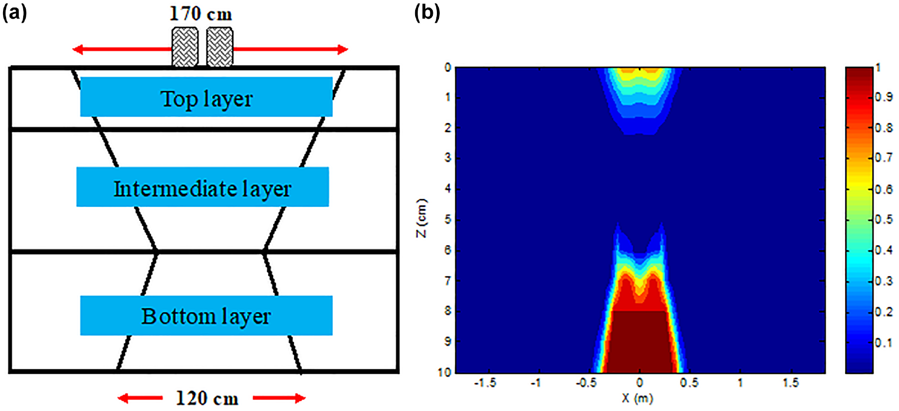
(a) Reference area for percentage damage definition in FlexPAVE™ and (b) damage contours representation.

It is important to highlight two advanced features included in CalME and FlexPAVE™ for fatigue cracking performance simulations. The first one is the approach of updating the pavement condition or damage with time caused by load and temperature effects, through an MLEA in CalME using the IR approach; and via FFE structural analysis in FlexPAVE™ using a nonlinear extrapolation scheme for damage accumulation. The second feature is the fatigue damage model that relates the damage characteristics of the AC directly to the performance of the pavement structure. This is through the damaged stiffness in CalME, and likewise, the S-VECD model is used by FlexPAVE™ to account for the fatigue damage. In contrast, the undamaged characteristics represented by the |E*| mastercurve are used as a surrogate model in Pavement ME to relate the fatigue damage to the pavement performance.

Figure 2 illustrates the different approaches for material properties variation during an analysis period employed by Pavement ME and CalME. In Pavement ME, modulus variation is dictated by aging/oxidation, temperature, and moisture content, as shown in Figure 2a. It is seen that the layers’ moduli vary seasonally under a constant range during the analysis period; an exception to this can be the upper part of the AC layer, which can show an increase in modulus values because of aging effects of the asphalt binder. Conversely, modulus variation in CalME is dictated by aging/oxidation, temperature, and damage, as shown in Figure 2b. It is seen that the layers’ modulus vary seasonally because of the temperature and the AC modulus initially increases because of aging but it then decreases as the damage grows during the analysis period. This temperature/damage variation of the AC layer influences the modulus variation of the unbound layers by acting as a plate applying a confining effect that changes with changes in AC stiffness, as well as the nonlinearity of the material (stress-dependence); to describe this modulus variation in the unbound layers Equation 31 is used ( 14 ).

E_{n} = E_{n, ref} \times [1 - (1 - \frac{S_{n}^{3}}{S_{ref}^{3}}) \cdot SF] \times {(\frac{P}{40 kN})}^{α}

(31)

where

E_n is the modulus of unbound layer n, counting from surface;

S_n is the bending stiffness for layer n (defined in Equation 32);

E_n,_ref is the modulus of layer n when bending stiffness is S = S_ref;

S_ref is the normalized bending stiffness, set to 3,500 MPa;

SF is the stiffness factor (model parameter);

P is the wheel load; and

α is a constant, which may be positive or negative depending on whether modulus increases or decreases with the wheel load.

S = \sum_{i = 1}^{n - 1} h_{n} \times \sqrt[3]{E_{n}}

(32)

where h_n is the thickness of the layer n.

Figure 2.

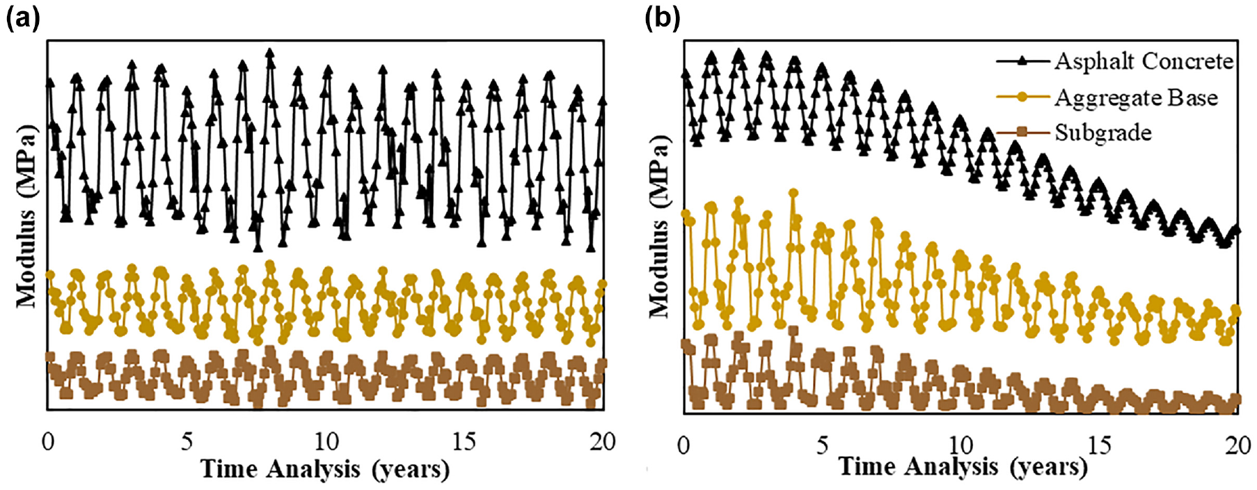
Schematic representation of material properties variation through the analysis period for: (a) pavement ME and (b) CalME.

The first part of the right-hand side of Equation 31 accounts for modulus variation as a function of confinement in the unbound layers from the layers above them. The second part describes the nonlinearity of unbound materials, modulus increasing with increasing of bulk stress for granular materials and modulus decreasing with increasing deviator stress. However, in CalME, this nonlinearity is treated as a function of the wheel load rather than as a function of the stress condition to avoid the interdependence between stiffness and stress. The detailed derivation of this model is described by Wu et al. ( 14 ).

In contrast, FlexPAVE™ 1.1 only accounts for the AC temperature and damage variation, as was explained before, but it does not consider the variation of the unbound layers. Therefore, unbound layers’ moduli are constant throughout the analysis period; for brevity, this behavior is not show in Figure 2.

Methodology

To prove the benefit of the features mentioned above, four laboratory-prepared AC mixtures were tested, and their properties were used to simulate the fatigue performance in a pavement study section. In this section, undamaged and damaged characteristics, as well as the details of the study section, are described.

Material Characterization

Four different mixtures, assembled with the same aggregate, gradation, asphalt content, and volumetric properties but using different asphalt binders, were tested to obtain the inputs to be used in the pavement performance simulations. The description of the asphalt binders employed, and the compaction temperatures of each mixture are shown in Table 1. To simulate short-term aging each mixture was stored for 4 h in an oven at the corresponding compaction temperatures according to AASHTO R 30 ( 23 ). Finally, the design gradation of 19 mm for the mixtures is shown in Figure 3.

Table 1.

Identification of the Asphalt Binders and Compaction Temperatures of the Mixtures

Mixture ID	Type of asphalt binder	Compaction temperature (°C)
PG64-16	Neat asphalt	145
PPA76H-16	PPA, Heavy traffic (H)^a	158
RET76E-22	Elvaloy^®+ PPA, Extreme traffic (E)^a	160
SBS76V-22	SBS + sulfur, Very heavy traffic (V)^a	165

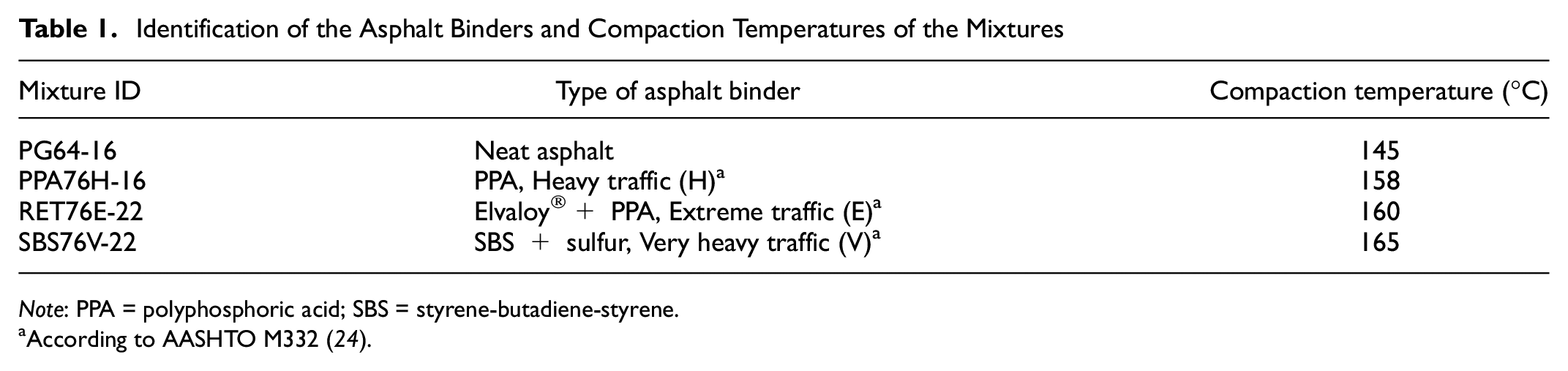
Note: PPA = polyphosphoric acid; SBS = styrene-butadiene-styrene.

According to AASHTO M332 ( 24 ).

Figure 3.

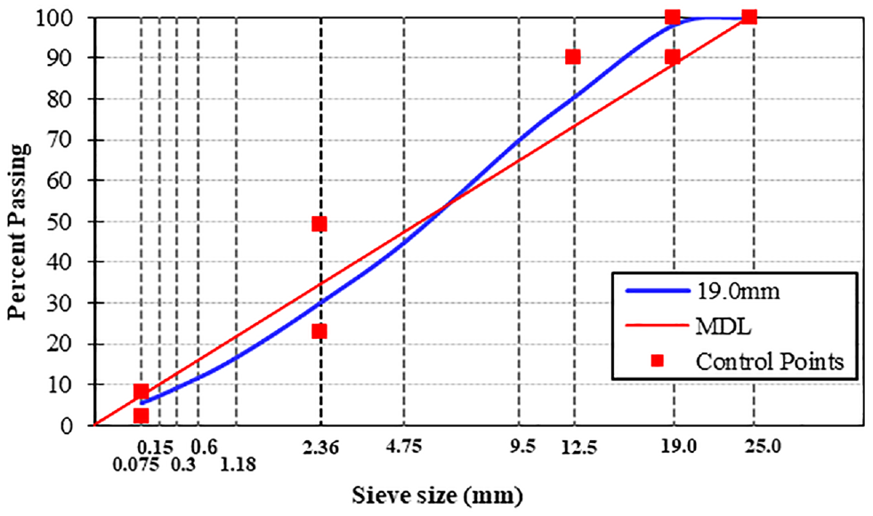
Design gradation for the asphalt mixtures represented by 0.45 power gradation chart.Note: MDL = maximum density line.

Undamaged Properties

Although in CalME the stiffness mastercurve parameters are typically obtained using data from frequency sweep testing on four-point bending beam specimens, in this study the stiffness mastercurves were obtained using the results from uniaxial sinusoidal tests, that is, tension-compression with zero mean waveforms. Three replicate samples were tested for each mixture to verify the repeatability, and they were subjected at six loading frequencies (25, 10, 5, 1, 0.5, 0.1 Hz) for each one of five temperatures (−10°C, 4°C, 20°C, 38°C, and 54°C).

The same |E*| data were processed in accordance with each methodology—for example, the stiffness mastercurves used in CalME were constructed using Equations 12 to 15 fixing the lower asymptote parameter to 200 MPa (δ = 2.301)—and the parameters of the optimization process are shown in Table 2. Similarly, the |E*| mastercurves used to compute the relaxation modulus mastercurves, Equation 21, required by FlexPAVE™ were constructed using Equations 22 and 23, and the results of the optimization process are also shown in Table 2.

Table 2.

Dynamic Modulus Mastercurves Parameters at a Reference Temperature of 20°C for the Different Study Mixtures and the Different ME Methodologies

Mixture	CalME parameters
Mixture	δ	α	β	γ	a_T	\|E\|_ref (MPa)* ^a	na
PG64-16	2.301	1.957	−0.415	0.821	1.060	5812	na
PPA76H-16	2.301	2.020	−1.085	0.624	1.201	9047	na
TER76E-22	2.301	2.004	−0.942	0.622	1.183	8132	na
SBS76V-22	2.301	3.044	−1.122	0.383	1.232	6304	na
Mixture	FlexPAVE™ 1.1 parameters
Mixture	d	a	b	g	a ₁	a ₂	a ₃
PG64-16	1.421	2.975	0.843	0.476	−0.00079	0.161	−2.910
PPA76H-16	0.511	4.000	1.530	0.321	−0.00047	0.158	−2.965
TER76E-22	0.970	3.495	1.336	0.345	−0.00066	0.168	−3.089
SBS76V-22	1.326	3.066	1.063	0.374	−0.00074	0.168	−3.064

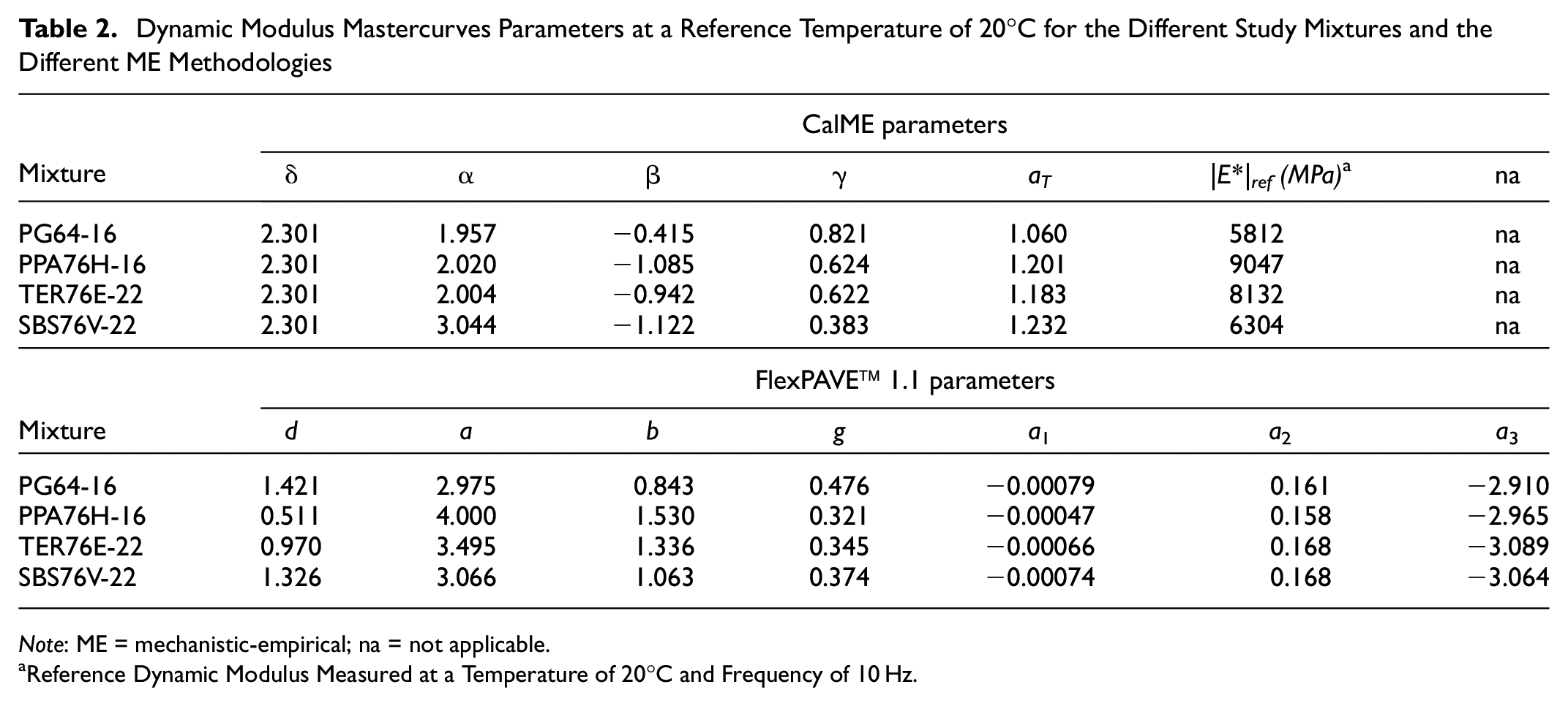
Note: ME = mechanistic-empirical; na = not applicable.

Reference Dynamic Modulus Measured at a Temperature of 20°C and Frequency of 10 Hz.

A representation of the |E*| mastercurves obtained with the distinct protocols is illustrated in Figure 4, where the asphalt mixtures that contain polyphosphoric acid (PPA) showed higher moduli. In contrast, the mixture with neat asphalt exhibited the lowest moduli for intermediate to low reduced times/frequencies. The exclusion of higher and lower modulus values using the CalME approach through fixing the lower asymptote of the mastercurve resulting from the symmetry of the sigmoidal model, can be seen in Figure 4a. The asymptotes are applied in CalME to reflect observed differences between laboratory values and field backcalculated values at low frequencies and high temperatures.

Figure 4.

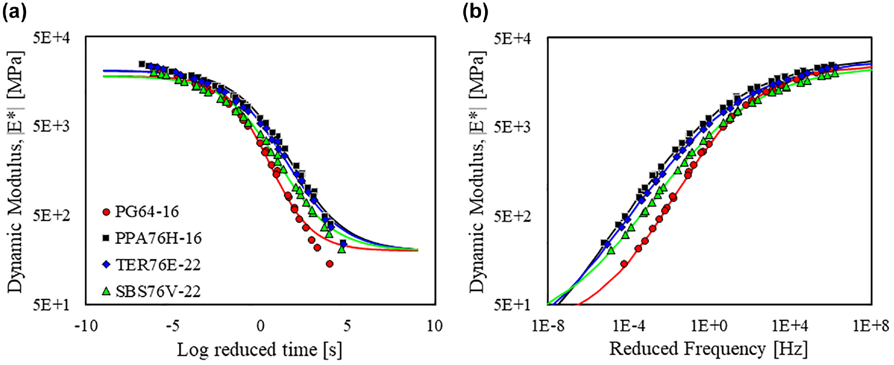
|E*| mastercurves constructed at a reference temperature of 20°C for the different asphalt mixtures, using (a) CalME and (b) FlexPAVE™ fitting procedures.

Fatigue Damaged Properties

Uniaxial cyclic fatigue tests were performed to obtain the damaged properties in accordance with AASHTO TP 107 ( 25 ). Then, the results were processed using the S-VECD model to simulate the stiffness degradation curves to be used in CalME and the damage characteristic curves to be used in FlexPAVE™; details about this procedure can be found elsewhere ( 26 ). It is well known that the uniaxial cyclic tests yield different fatigue damage lives than the four-point bending beam fatigue tests. In this article, the stiffness reduction curves were simulated using the S-VECD model for three distinct strain levels (200, 500, and 800 µε) to initially calibrate the fatigue damage parameters required by CalME, and the transfer function was then calibrated using field performance data. The damage parameters used by the fatigue model in CalME, Equations 16 to 18, as well as the parameters required by the damage calculation in FlexPAVE™, Equations 25 to 27, are presented in Table 3.

Table 3.

Fatigue Damage Parameters of the Study Mixtures Used in CalME and FlexPAVE™

Mixture	CalME parameters
Mixture	A	β	γ	α ₀
PG64-16	539.4	−6.326	−3.163	−1.187
PPA76H-16	2708.6	−6.264	−3.132	−1.195
TER76E-22	38715.1	−7.224	−3.612	−1.390
SBS76V-22	11030.8	−6.199	−3.099	−1.330
Mixture	FlexPAVE™ 1.1 parameters
Mixture	α	C ₁₁	C ₁₂	D ^R
PG64-16	3.554	0.00215	0.519	0.477
PPA76H-16	3.922	0.00177	0.500	0.440
TER76E-22	3.971	0.00235	0.473	0.470
SBS76V-22	4.120	0.00564	0.417	0.610

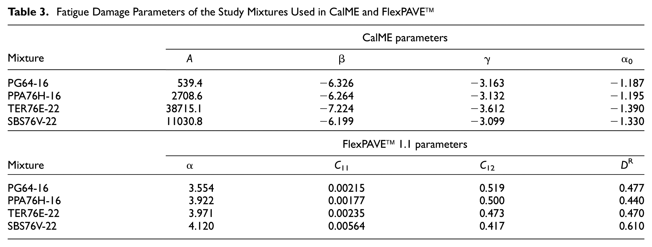
The fatigue damage curves used as input by each methodology coming from the S-VECD model are illustrated in Figure 5. It is noteworthy from the curves in Figure 5 that the polymer-modified mixtures (TER76E-22, and SBS76V-22) show better fatigue life than unmodified (PG64-16) and polyphosphoric acid (PPA76H-16) mixtures under controlled strain conditions of simulation.

Figure 5.

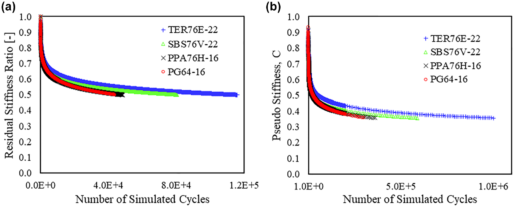
Comparison of the fatigue damage curves for the different mixtures obtained from uniaxial cyclic tests using the S-VECD model: (a) normalized stiffness reduction and (b) pseudo stiffness.

Study Section

The overall location for the study section, which is in Tizayuca County, Hidalgo State, Mexico, is shown in Figure 6a. The road test section has connections to an extensive regional road network, as is illustrated in Figure 6b. This study section has a length of 3.4 km, and it was reconstructed and widened to two lanes in each direction in 2012. This section was chosen because the information about its performance since then is available. Table 4 presents the characteristics of the pavement design obtained from the bidding process.

Figure 6.

(a) localization of the test section and (b) connectivity details with other important roads in Mexico.

Table 4.

Pavement Structure Characteristics Reconstructed in 2012

Layer type	Description	Thickness (mm)	Mexican standard
Asphalt concrete	Dense gradation, NMAS 19 mm, unmodified PG64-16	100	N-CMT-4-05-003-08
Aggregate base	Well-graded gravel with a CBR minimum of 100%	250	N-CMT-4-02-002-11
Subgrade	Silty clay with a CBR minimum of 20%	na	N-CMT-1-03-02

Note: NMAS = nominal maximum aggregate size; CBR = California bearing ratio; na = not applicable.

Traffic and Climate Data

The traffic volume and the truckload distribution were extracted from data provided by the Technical Services General Directorate (DGST) website, http://www.sct.gob.mx/. Using this information, data were collected based on the input requirements of the two methodologies. A value of 10.5% annual truck traffic growth was estimated from the annual average daily truck traffic. CalME uses an axle load spectrum concept, which is defined based on the frequency of different axle loads by axle type over 24-h periods, as shown in Figure 7a. Also, the total number of truck axles accumulated in the first year of simulation is required. The yearly total axle count will then be evenly distributed over each day based on the axle load spectrum; a value of 1,104,400 axle repetitions was used as input. Conversely, in FlexPAVE™, all the traffic data are converted into the number of passes of a standard axle (two dual tires with an 80 kN axle load) with a constant speed (25 m/s) based on the design equivalent single-axle loads (ESALs); the figure of 2,130 daily ESALs was used as input.

Figure 7.

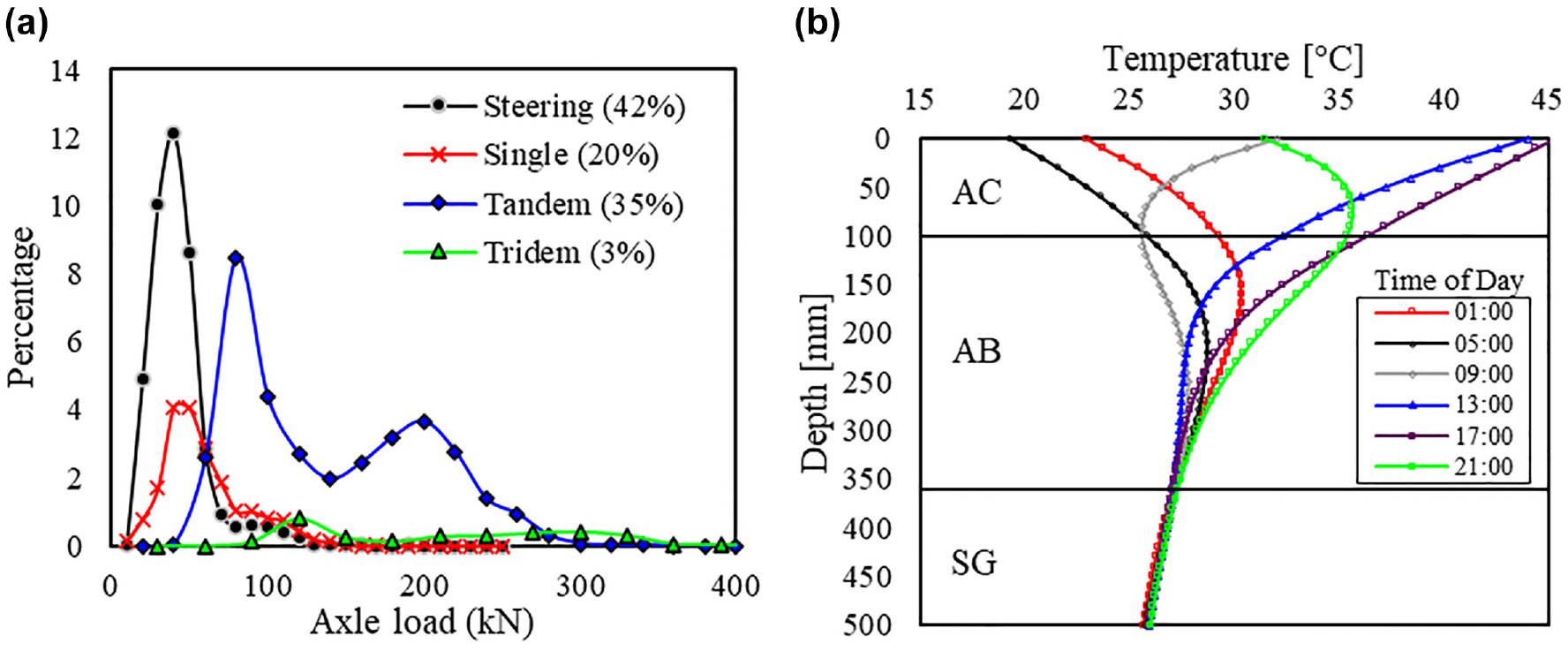
(a) Axle load spectra (including the percentage of total axles in the legend) and (b) pavement temperature-depth profile for May 28, 2012, in 4-h intervals.

The information on the environmental conditions was obtained from the website of the Long-Term Pavement Performance MERRA Climate Data for MEPDG Inputs (https://infopave.fhwa.dot.gov/), which has a spatial resolution of approximately 50 by 60 km. The nearest station available was Cell 121091 (latitude 20.0, longitude −98.75), which is only 20 km from the study section. Conversely, the nearest climatic station from the Mexican climatic database (http://siclic.imt.mx/) is 25 km from the study section but it only has available daily environmental data, which are not adequate for the pavement temperature simulations. Using Cell 121091 data, the pavement temperature profile was calculated using TEMPS (Temperature Estimate Model for Pavement Structures) software, developed by the University of Nevada, Reno (http://www.arc.unr.edu/TEMPS). Figure 7b shows the temperature distribution for the hottest day of 2012 in 4-h intervals. The hourly surface temperatures calculated using data from a 30-year period were stored in the CalME temperature database to predict the temperature profile during the performance simulations. Similarly, the temperature profile calculated using TEMPS was introduced in FlexPAVE™ and used to simulate pavement performance.

Performance

The structural and surface condition of the study section was supplied by DGST, and from this information, the elastic modulus of the different layers was computed using the Falling Weight Deflectometer (FWD) measurements for each survey campaign via backcalculation of stiffnesses using the CalBack software ( 27 ). The structural capacity evolution of the pavement is illustrated in Figure 8a, where elastic modulus degradation can be observed arising from the combination of the high level of traffic loads repetitions and the thinness of the AC layer. It should be highlighted that only the backcalculated modulus values of the unbound layers for the 2012 year were used as input in the simulations, because the different laboratory mastercurves shown in Figure 4 were used.

Figure 8.

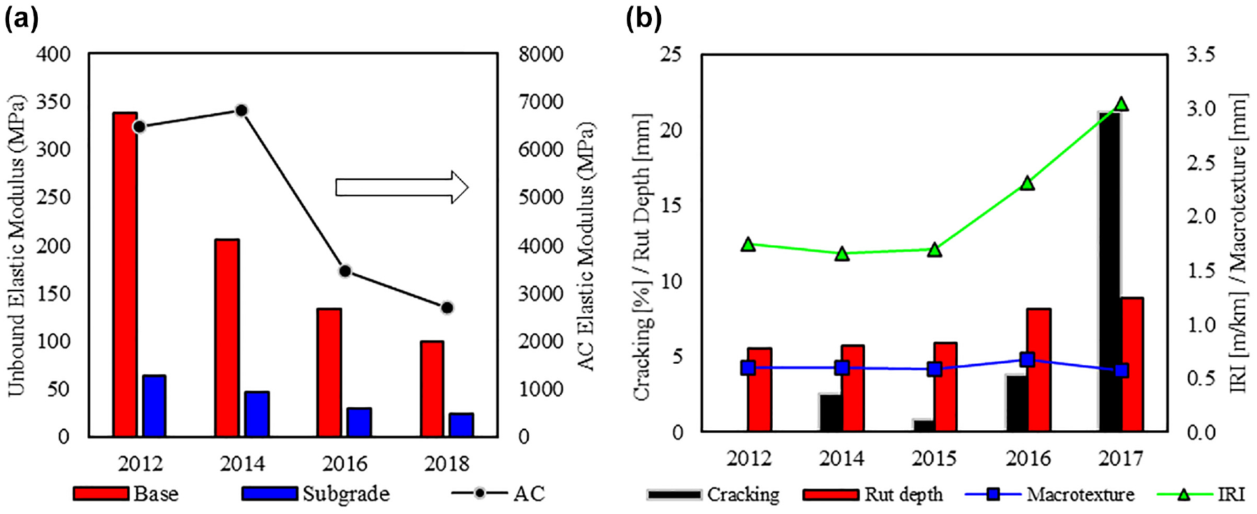
Structural and surface conditions of the pavement study section for the different survey campaigns: (a) pavement layers average elastic modulus (AC modulus was normalized to 20°C) and (b) median values of the surface characteristics.

The surface condition of the pavement is shown in Figure 8b, where fatigue cracking distress dominates the damage to the AC, and it can be related to the stiffness degradation observed in the elastic modulus evolution (Figure 8a). It should be emphasized that this fatigue cracking represents the field cracking measured in the total lane. For purposes of the transfer function calibrations, it was converted to the cracking in the wheel paths, multiplying by a factor of two the field cracking since the wheel path area is considered as half of the area of the total lane surface.

Results and Discussion

The results of the pavement performance simulations are presented in this section. First, the undamaged and damaged AC properties of the unmodified mixture (PG64-16) were used to calibrate the transfer functions, adjusting the empirical parameters to match the predicted cracking against the observed field cracking. Then, the properties of the AC were changed using the other mixture characteristics to perform the pavement simulations. The primary purpose of changing the AC mixtures is to evaluate the impact of fatigue cracking performance using modified binders.

The decision to use the unmodified mixture as a baseline condition to calibrate the transfer function parameters against the field cracking was made on the assumptions that the basalt aggregate is from a source close to the study section location, the PG64-16 asphalt was produced in a refinery close to the study section, and, finally, the aggregate gradation is commonly used in the Metropolitan Valley of Mexico. All those attributes made it probable that the unmodified mixture represents the characteristics of the original AC used in the reconstruction of the study section, which are described in Table 4.

CalME 2.0 Simulations

The transfer function calibration was achieved, changing the parameters α₁ and α₂ in Equations 19 and 20, respectively. These parameters represent the cracking rate for initiation and progression conditions; the value of α₁ was changed from −2 to −1.1, and α₂ was changed from −8 to −24, meaning that the field cracking in the study section initiated more slowly and propagated at a slower rate than the simulations performed with the original values. Subsequently, simulations for the different AC mixtures were carried out. Figure 9a shows the fatigue damage evolution for the distinct AC mixtures. As seen, damage growth was faster for unmodified and PPA mixtures in comparison with the polymer-modified ones, and the difference in damage evolution between the last ones is slight.

Figure 9.

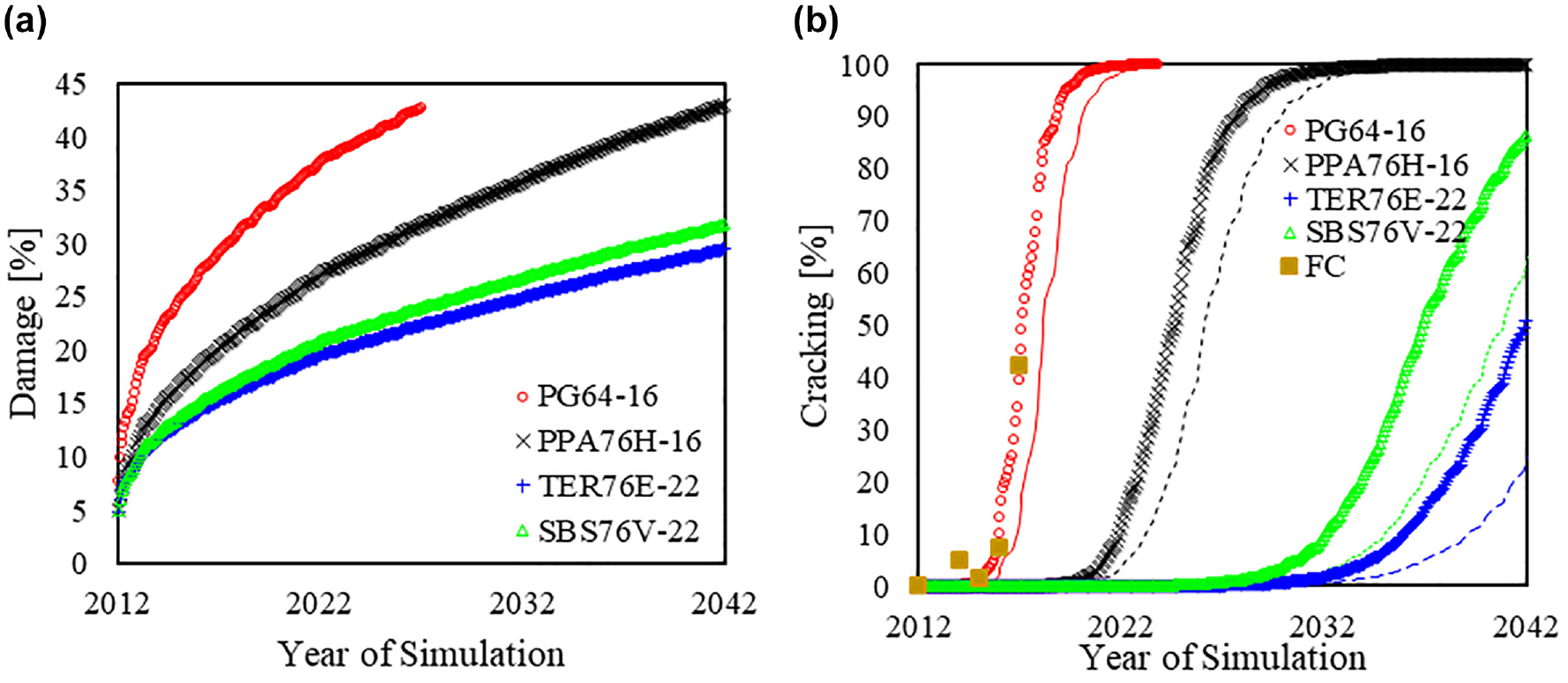
Pavement fatigue performance simulations for the different AC mixtures using CalME: (a) damage and (b) cracking (including field cracking, FC).

Figure 9b presents the fatigue cracking simulations for the different AC mixtures. In this figure, the simulated cracking matches the field cracking (FC) because of the calibration process. Symbols in Figure 9b represent simulations performed in deterministic mode, and lines represent the average of 20 simulations performed in probabilistic mode. The observations of primary interest are that the cracking curves take a longer time to initiate and progress on modified mixtures, even for the PPA mixture, which previously has shown similar fatigue resistance to the unmodified mixture (see Figure 5). This cracking improvement can be attributed to the higher stiffness of the PPA mixture (see Figure 4). Additionally, polymer-modified mixtures show higher fatigue cracking resistance. However, the fatigue cracking curves seem excessively elongated for the thin AC layer in the study section, yielding less than 20% cracking for more than 20 years, which may be attributed to very few polymer-modified mixtures used in CalME development.

FlexPAVE™ 1.1 Simulations

The parameters C_f₁, C_f₂, and C_f₃ from Equation 30 were adjusted to calibrate the fatigue damage transfer function. These values were changed from 0.342 to 0.15, from 13.97 to 95, and from 16.38 to 20, respectively. The change of these values reflects a decrement in the cracking initiation and progression rate simulations to adjust to the field pavement conditions. This behavior agrees with CalME simulations using default values, but FlexPAVE™ results showed faster cracking initiation and progression rates. The damage growth for the different AC mixtures is shown in Figure 10a. The shape and the trend of the damage curves are consistent with CalME simulations, although there are some differences in the damage evolution between the different mixtures. The polymer-modified mixtures show lower damage growth, the same as for the CalME damage predictions.

Figure 10.

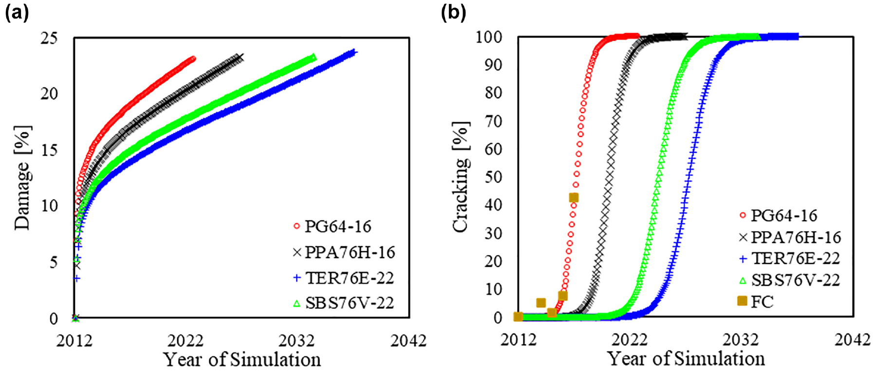
Pavement fatigue performance for the different AC mixtures using FlexPAVE™: (a) damage and (b) cracking (including field cracking, FC).

Figure 10b depicts the fatigue cracking simulations for the different AC mixtures. Similarly, there is a superposition among the simulated and observed cracking after calibration. Additionally, modified mixtures show higher fatigue cracking resistance in comparison with the unmodified ones; however, the time to develop 20% cracking is significantly less than in CalME simulations and seems to be more realistic for a thin AC layer.

The discrepancy between the cracking evolution for CalME and FlexPAVE™ could be attributed mainly to two different aspects. The first of these is the distinct approach to considering traffic loads taken by each software system. Damage accumulation can be different when using a single axle (ESAL) configuration and fixed axle load (80 kN), as is defined by FlexPAVE™, compared with the damage accumulation using different axle types (steering, single, tandem, and tridem) and varying axle loads (spectra) as defined by CalME. Additional influences on the damage accumulation may have included other input assumption differences such as tire pressure and contact area: FlexPAVE™ uses a tire pressure of 827 kPa and a rectangular contact area shape (28 cm length and 18.8 cm width) as default parameters. Conversely, CalME uses a constant tire pressure of 690 kPa for both single and dual wheels with a circular contact area described by a constant radius of 12 cm for single and 11.2 cm for dual wheels.

It is believed that these differences are related to the large divergences in the fatigue performance predictions of the modified mixtures. For example, considering a single axle with dual wheels, CalME distributes the load from 10 to 130 kN (as shown in Figure 7a) into five periods to compute the horizontal strain at the bottom of the AC using temperature average for each period, and then the damage is accumulated for each axle load repetition based on the axle number for the first year and the axle spectrum. In contrast, FlexPAVE™ computes the response (horizontal strain) at the bottom of the AC layer using the same axle load (80 kN) and accumulates the damage for fixed daily load applications distributed in each one of the three analysis segments, using each segment’s average temperatures. Thus, this constant load may lead to higher damage accumulation and therefore faster cracking development in comparison with CalME simulations. If the other axle types are considered, the damage may be similar or lower for tandem and tridem axles, because of the load range (40–300 kN for tandem, and 80–400 kN for tridem) being distributed on a higher number of axles. Conversely, the steering axle may cause higher damage because the load of 10–140 kN (as shown in Figure 7a) is distributed on a single wheel. However, the number of load applications of each axle type for damage accumulation depends on the axle number for the first year and the load spectra; thus the accumulated damage and the fatigue cracking may be lower in comparison with a fixed load and load repetitions, as is shown in Figures 9 and 10.

The second aspect is the effect of the unbound layers’ nonlinearity on the critical response (horizontal strain at the bottom of AC layer). Several studies ( 28 – 32 ) highlighted the importance of incorporating the operational conditions (e.g., moisture, stress-nonlinearity, and anisotropy) of unbound layers into the pavement analysis/design methodologies. Some of these studies ( 30 – 32 ) point out that excluding stress-dependent behavior of unbound layers could cause underestimation of the critical responses of flexible pavement structures and, therefore, higher estimated pavement life for rutting and fatigue cracking. CalME uses Equation 31 to describe the behavior of unbound layers under temperature-induced stiffness changes of the AC layers affecting confinement, and traffic load. Conversely, FlexPAVE™ uses constant moduli for unbound layers; however, opposite to the findings in the literature, the incorporation of the nonlinear behavior in CalME did not result in lower fatigue performance in comparison with FlexPAVE™ (which does not consider the nonlinear effects). A possible explanation of these results is the different approach to simulating the AC behavior: linear elastic for CalME and linear viscoelastic for FlexPAVE™. It is worth noting that the references cited ( 30 – 32 ) used a linear viscoelastic model to simulate the AC behavior and considered the cross-anisotropic stress-dependent modulus for unbound layers. Because none of the methodologies used in this research fulfill these criteria, it is concluded that the effect of the load dominates the damage growth for fatigue cracking performance, resulting in higher damage for a constant load axle in comparison with load spectra and axle configurations, before the field calibrations for the unmodified mixture and after the calibration for the modified mixtures.

The advantage of the additional features in the second-generation analysis engines has been demonstrated in the above fatigue performance simulations. However, notwithstanding the enhancements in damage evolution, the progress of the distress models for AC, and higher computation efficiency, these approaches are far from finalized in their development. Therefore, based on a continuous improvement framework both research groups are working on the next version of the analysis engines, and the most important features are discussed below.

CalME 3.0 is now a web-based application, where the performance prediction models are enhanced through a new comprehensive calibration approach to consider the performance variability using “big data” for performance from thousands of test sections in the Caltrans Pavement Management System (PaveM) and state-wide median material properties. The performance variability is accounted for through within-project variability (WPV) and between-project variability (BPV). In this approach PaveM data are grouped in cells with the same AC thickness and traffic characteristics but distinct performance for calibration and validation purposes. The BPV is caused by uncertainties in materials and traffic, and it is determined as the distribution of the ratio between the time to reach 50% field performance damage (t₅₀) expressed as cracking or rutting to the time to reach 50% predicted damage (t_ω50) for each calibration cell. The WPV includes the variation in performance distress models, layer thicknesses, and layer stiffnesses within a given project, and it is determined as the shape of the percentage failure time history, which is the normalization of the pavement age by dividing the actual age by the corresponding t₅₀, and multiplying it by t_ω50. At the time that this paper was written this new version was only available for California road network analysis.

FlexPAVE™ 2.0 is currently under finalized development. This version of the software will maintain the primary functionality of FlexPAVE™ 1.1 but includes numerous enhancements. First, the graphical user interface will be substantially simplified and will integrate more seamlessly with the FlexMAT™ material analysis tool. In addition, the overall pavement response engine is being updated to increase accuracy and computational efficiency. This improved efficiency will allow a more robust climate dataset covering multiple years and allow for seasonally varying unbound layer properties. The response will also be recursive with the damage calculations instead of being independent of those damage calculations. Additionally, since the pavement response model will be based on Fourier analysis, the linear viscoelastic material model will be modified to include the 2S2P1D complex modulus model. Finally, surrogate models to account for aging, thermal stresses, and the combination of thermal and load associated stresses will be incorporated.

Conclusions

In this article, a comprehensive review of three pavement damage models is first presented, using fatigue damage models as an example, and the additional features of CalME 2.0 and FlexPAVE™ 1.1 over Pavement ME are highlighted. The process of damage accumulation and a closer linkage of the mechanical material properties with the pavement performance evolution are the most important features shown.

The capabilities of the features mentioned above were demonstrated by simulating the fatigue performance for a study pavement section, using laboratory-prepared specimens for four AC mixtures with similar characteristics but distinct mechanical properties. The transfer functions of the ME tools were first calibrated against field cracking, using the AC properties of the unmodified mixture to perform cracking predictions. Then, fatigue damage simulations for the other mixtures were carried out. The results showed a similar ranking in fatigue cracking performance for both CalME and FlexPAVE™ simulations. Modified mixtures exhibited more fatigue cracking resistance in comparison with the unmodified mix, but the polymer-modified ones shown higher fatigue damage resistance. But a longer time to fatigue damage development was observed in CalME simulations, in comparison with FlexPAVE™ predictions that presented faster initiation and higher progression rates during fatigue cracking evolution before and after calibration. However, the cracking predictions for polymer-modified mixtures in CalME seem to be unrealistically long for the thin AC thickness in the study section. Two different aspects were analyzed to explain the discrepancy in the fatigue performance simulations—the different approach to considering traffic loads and the effects of nonlinearity of unbound layers’ stiffnesses on the critical pavement response. It is believed that the different approach to considering traffic loads—single axle with constant load in FlexPAVE™ and axle spectrum varying load in CalME—is the main factor that influences the damage growth in the simulations.

Finally, current, and future enhancements of both approaches based on a continuous improvement framework are briefly discussed.

Footnotes

Acknowledgements

The authors gratefully acknowledge the support of the DGST in providing the pavement performance data, the University of California Pavement Research Center in providing the software CalME, and the Pavement Research Team from North Carolina State University in providing the software FlexPAVE™.

Author Contributions

The authors confirm contribution to the paper as follows: study conception and design: N. Hernandez-Fernandez, J. Harvey, S. Underwood, and A. Ossa-Lopez; data collection: N. Hernandez-Fernandez; analysis and interpretation of results: N. Hernandez-Fernandez, J. Harvey, S. Underwood, and A. Ossa-Lopez; draft manuscript preparation: N. Hernandez-Fernandez, J. Harvey, S. Underwood, and A. Ossa-Lopez. All authors reviewed the results and approved the final version of the manuscript.

Declaration of Conflicting Interests

The author(s) declared no potential conflicts of interest with respect to the research, authorship, and/or publication of this article.

Funding

The author(s) received no financial support for the research, authorship, and/or publication of this article.

ORCID iDs

John T. Harvey

Benjamin Shane Underwood

Alexandra Ossa-Lopez

References

American Association of State Highway and Transportation Officials. Pavement Design, Construction, and Management: A Digital Handbook. AASHTO, Washington, D.C., 2015.

Ahmed

Erlingsson

Viscoelastic Response Modelling of a Pavement under Moving Load. Transportation Research Procedia, Vol. 14, 2016, pp. 748–757. https://doi.org/10.1016/j.trpro.2016.05.343.

Pereira

Pais

Main Flexible Pavement and Mix Design Methods in Europe and Challenges for the Development of an European Method. Journal of Traffic and Transportation Engineering (English Edition), Vol. 4, No. 4, 2017, pp. 316–346. https://doi.org/10.1016/j.jtte.2017.06.001.

COST 333. Development of New Bituminous Pavement Design Method. Luxembourg, 2000.

ARA, Inc., ERES Consultants Division. Guide for Mechanistic-Empirical Design of New and Rehabilitation Pavement Structures. Final Report, NCHRP Project 1-37A. Transportation Research Board of the National Academies, Champaign, IL, 2004.

Xiao

D. X.

Wang

K. C. P.

Hall

K. D.

Qiu

Mechanistic-Empirical Pavement Design Guide (MEPDG): A Bird’s-Eye View. Journal of Modern Transportation, Vol. 19, No. 2, 2011, pp. 114–133. https://doi.org/10.1007/bf03325749.

Yuan

X. X.

Nemtsov

Local Calibration of the MEPDG Distress and Performance Models for Ontario’s Flexible Roads: Overview, Impacts, and Reflection. Transportation Research Record: Journal of the Transportation Research Board, 2018. 2672: 207–216.

Caliendo

Local Calibration and Implementation of the Mechanistic-Empirical Pavement Design Guide for Flexible Pavement Design. Journal of Transportation Engineering, Vol. 138, No. 3, 2012, pp. 348–360. https://doi.org/10.1061/(ASCE)TE.1943-5436.0000328.

Ullidtz

Harvey

Basheer

Jones

Lea

CalME, a Mechanistic-Empirical Program to Analyze and Design Flexible Pavement Rehabilitation. Transportation Research Record: Journal of the Transportation Research Board, 2010. 2153: 143–152.

10.

Eslaminia

Thirunavukkarasu

Guddati

M. N.

Richard Kim

Accelerated Pavement Performance Modeling Using Layered Viscoelastic Analysis. In 7th RILEM International Conference on Cracking in Pavements ( Scarpas

Kringos

Al-Qadi

Loizos

, eds.), Springer, Dordrecht, 2012, pp. 497–506.

11.

American Association of State Highway and Transportation Officials. Mechanistic-Empirical Pavement Design Guide: A Manual of Practice. AASHTO, Washington, D.C., 2015.

12.

AASHTO Designation. AASHTO R 62: Standard Practice for Developing Dynamic Modulus Master Curves for Asphalt Mixtures. AASHTO, Washington, D.C., 2013, p. 9.

13.

ASTM International. ASTM D2493-16: Standard Practice for Viscosity-Temperature Chart for Asphalt Binders. ASTM International, West Conshohocken, PA, 2016.

14.

Zhou

Harvey

J. T.

Update CalME Standard Materials Library. Report No. UCPRC-TM-2014-8. Institute of Transportation Studies, University of California, Davis, 2018.

15.

Ullidtz

Mateos

Ayuso

Harvey

Basheer

Simulation of Full Scale Accelerated Pavement Test from CEDEX Using the Californian Predictive Pavement Design System (CalME). Proc., 11th International Society for Asphalt Pavements (ISAP), Nagoya, Japan, 2010.

16.

Lea

J. D.

Harvey

J. T.

Simplified Thermal Modeling Approach Used in CalME. Presented at 91st Annual Meeting of the Transportation Research Board, Washington, D.C., 2012.

17.

. Calibration of CalME Models Using Field Data Collected from US 101 near Redwood National Park, Humboldt County. Report No. UCD-ITS-RR-08-09. Institute of Transportation Studies, University of California, Davis, 2008.

18.

Eslaminia

Guddati

M. N.

Fourier-Finite Element Analysis of Pavements under Moving Vehicular Loading. International Journal of Pavement Engineering, Vol. 17, No. 7, 2016, pp. 602–614. https://doi.org/10.1080/10298436.2015.1007237.

19.

Cao

Norouzi

Kim

Y. R.

Application of Viscoelastic Continuum Damage Approach to Predict Fatigue Performance of Binzhou Perpetual Pavements. Journal of Traffic and Transportation Engineering (English Edition), Vol. 3, No. 2, 2016, pp. 104–115. https://doi.org/10.1016/j.jtte.2016.03.002.

20.

Baek

C. M.

Top-Down Cracking Mechanisms Using the Viscoelastic Continuum Damage Finite Element Program. PhD dissertation. North Carolina State University, Raleigh, 2010.

21.

Wang

Y. D.

Keshavarzi

Kim

Y. R.

Fatigue Performance Prediction of Asphalt Pavements with FlexPAVE™, the S-VECD Model, and D^R Failure Criterion. Transportation Research Record: Journal of the Transportation Research Board, 2018. 2672: 217–227.

22.

Wang

Y. D

. Development of the Framework of Performance-Engineered Mixture Design for Asphalt Concrete. PhD dissertation. North Carolina State University, Raleigh, 2019.

23.

AASHTO Designation. AASHTO R 30-02. Standard Practice for Mixture Conditioning of Hot-Mix Asphalt (HMA). AASHTO, Washington, D.C., 2015, p. 5.

24.

AASHTO Designation. AASHTO M 332: Standard Specification for Performance-Graded Asphalt Binder Using Multiple Stress Creep Recovery (MSCR) Test. AASHTO, Washington, D.C., 2010.

25.

AASHTO Designation. AASHTO TP 107-14: Standard Method of Test for Determining the Damage Characteristic Curve of Asphalt Mixtures from Direct Tension Cyclic Fatigue Tests. AASHTO, Washington, D.C., 2014, p. 48.

26.

Hernandez-Fernandez

Underwood

B. S.

Ossa-Lopez

Simulation of the Asphalt Concrete Stiffness Degradation Using Simplified Viscoelastic Continuum Damage Model. International Journal of Fatigue, Vol. 140, 2020, p. 105850. https://doi.org/10.1016/j.ijfatigue.2020.105850.

27.

Ullidtz

Basheer

Ghuzlan

Signore

J. M.

CalBack: Enhancing Caltrans Mechanistic-Empirical Pavement Design Process with New Back-Calculation Software. Journal of Transportation Engineering, Vol. 135, No. 7, 2009, pp. 479–488. https://doi.org/10.1061/(ASCE)TE.1943-5436.0000010.

28.

Erol

State of the Art: Anisotropic Characterization of Unbound Aggregate Layers in Flexible Pavements. In Symposium on Pavement Mechanics and Materials at the Inaugural International Conference of the Engineering Mechanics Institute, Minneapolis, MN, 2008.

29.

Luo

Zhang

Lytton

R. L.

Zollinger

Mechanistic-Empirical Models for Better Consideration of Subgrade and Unbound Layers Influence on Pavement Performance. Transportation Geotechnics, Vol. 13, 2017, pp. 52–68. https://doi.org/10.1016/j.trgeo.2017.06.002.

30.

Wang

Al-Qadi

I. L.

Importance of Nonlinear Anisotropic Modeling of Granular Base for Predicting Maximum Viscoelastic Pavement Responses under Moving Vehicular Loading. Journal of Engineering Mechanics, Vol. 139, No. 1, 2013, pp. 29–38. https://doi.org/10.1061/(asce)em.1943-7889.0000465.

31.

Al-Qadi

Wang

Tutumluer

Dynamic Analysis of Thin Asphalt Pavements by Using Cross-Anisotropic Stress-Dependent Properties for Granular Layer. Transportation Research Record: Journal of the Transportation Research Board, 2010. 2154: 156–163.

32.

Wang

Evaluation of Effects of Variations in Aggregate Base Layer Properties on Flexible Pavement Performance. Transportation Research Record: Journal of the Transportation Research Board, 2015. 2524: 119–129.