Utilization and Cost Estimation Models for Highway Fleet Equipment

Abstract

Highway agencies need to manage the utilization of their highway equipment assets to reduce fleet management costs, balance equipment use, and provide the required services. Predictive equipment utilization and operational cost models are required for optimal management; however, there are no widely accepted models for this purpose. Although the utilization data is collected by state DOTs, the literature does not show any specific statistical model to predict equipment utilization as a function of contributing factors such as asset age, fleet size, costs, and demand for service. This study will bridge this gap and develop a predictive model to estimate the utilization of fleet equipment. The main objective of this paper is to develop a set of predictive models to estimate the annual utilization of seven non-stationary highway equipment types based on several explanatory variables including their annual fuel cost, downtime hours, age, and weight. Furthermore, another set of models are fit to predict the annual operational cost for these equipment types based on the most important contributing factors. The prediction models are developed after a nationwide data collection. Several years of collected data from seven states are processed and used for model development. This research has identified annual mileage as an appropriate and widely used utilization metric. Various model structures to predict annual mileage are considered. The logarithmic function of annual mileage has provided the most appropriate structure. The final annual mileage predictive models have R-squared values that are between 0.65 and 0.89, which indicates a good fit for all models. The models are validated by performing several statistical tests and they have satisfied all required assumptions of regression analysis. The result of modeling and statistical analysis showed that the proposed models accurately estimated the utilization and operational cost for highway equipment assets.

Proper management of equipment fleet assets can lead to significant cost reductions for highway agencies and potential benefits in environmental stewardship. The significant capital investments associated with operations equipment assets mean that long-term planning for utilization, maintenance, and replacement activities is essential ( 1 , 2 ). Developing accurate predictive models will estimate the utilization and operational costs based on a range of contributing factors and help support such management activities ( 3 , 4 ). There is a need to identify the most appropriate utilization metrics, contributing factors to utilization, and predictive models to estimate the utilization and operational cost of equipment.

Various procedures are employed in practice that aim to address the utilization measurement and management challenges for highway agencies (5 –7). Historical data are used to estimate the cost and utilization of highway fleet assets ( 8 ). Aggregated data could provide supervisory perspectives to the highway agency’s fleet, while disaggregated data are helpful for a better operational performance of each equipment unit. However, there is no widely accepted process for determining utilization criteria, measurement metrics, and the most important contributing factors to utilization.

The objective of this research is to determine the most appropriate utilization metrics, contributing factors to utilization, and predictive models to estimate utilization. It also develops models for operational cost prediction of highway fleet equipment. This paper focuses on seven non-stationary equipment types: dump trucks, pickup trucks, automobiles, vans, sport utility vehicles, truck tractors, and large trucks with a special body. After determining the most important factors, the research team undertook a national data collection effort and collected four years of equipment utilization and cost data from seven states across the U.S.A. The data was then processed, and utilization measurement and operational cost predictive models were fit and validated. In the remainder of this paper, a review of the literature, data collection plan, data processing, model fitting, model validation, and the results are presented.

Background

The background section focuses on asset utilization measurement techniques that are used by the transportation agencies in several state departments of transportation (DOT) to find the most important factors that can affect fleet utilization. Ohio Department of Transportation (ODOT) ( 9 ) categorizes its equipment based on the general asset value, widespread use across the state, and the number of pieces. The main category includes two separate groups of heavy equipment, which contains equipment that is primarily used for construction and maintenance activities. ODOT uses annual engine hours and mileage as utilization metrics for different categories of equipment under seasonality constraints.

The City of San Bernardino ( 10 ) recommended some standards for categorizing equipment fleet assets and measuring the utilization of the functional classes. The City’s vehicle and equipment fleets were categorized into seven functional categories under two broad classifications: “general use” and “special use.” The utilization measures included monthly average miles or hours, which helped identify the over- or under-utilized units in comparison with the developed minimum utilization standard for potential reassigning or disposal. Moreover, the fleet size reduction, makeup adjustment, and the number of pool units were considered based on an estimate of their salvage value, estimated annual maintenance and repair cost savings, and replacement cost savings.

Minnesota Department of Transportation (MnDOT) ( 11 ) provided fleet management performance measures that targeted equipment utilization, units out-of-life cycle, fleet size, and scheduled versus unscheduled maintenance. The state has established a set of “equipment utilization rate goals” for mobile equipment assets including all light, medium, and heavy-duty vehicles. Moreover, the minimum utilization requirements for different types of assets were identified based on their usage in different seasons. The key factors that influenced equipment utilization and management strategies were the annual mileage, annual engine hour, and seasonality.

Utah Department of Transportation (UDOT) ( 12 ) has improved its utilization management by monitoring equipment effectively through its Division of Fleet Operations vehicle information system. The key factors in equipment utilization management at UDOT included the mileage per month, frequency of use, and purpose/need for vehicles that did not meet mileage and frequency of use criteria. The study on UDOT’s fleet suggested that renting the seasonal and low utilization equipment would be cost-effective if it were feasible.

California Department of Transportation (CalTrans) used several fleet performance measures, which include utilization, preventive maintenance, retention, and availability/downtime for fleet management ( 13 ).

Texas Department of Transportation (TxDOT) ( 14 ) conducted a performance measure preventive maintenance study for a single category of equipment assets. Using the FleetTrackS program, the state tracked the utilization measures over time based on engine data collected through an onboard diagnostic system. The collected data from the engine were based on the vehicle mile or operational hours. Moreover, TxDOT ( 15 ) used some usage measures such as equipment’s age, mileage, resale value, and repair cost to decide about replacement. TxDOT used its Texas Equipment Replacement Model (TERM) to manage equipment replacement and plan for future needs. Using TERM, the state identified candidate equipment units for replacement one year ahead. TxDOT’s TERM2 ( 16 ) improved the previous model with enhanced functionalities and considering several factors such as future uncertain purchase costs, unavailability of funds, and disaster preparedness.

South Carolina Department of Transportation (SCDOT) ( 17 ) developed its Transportation Equipment Replacement Model System (TERMS) based on TxDOT’s source code (TERM) to manage equipment and provide reliable equipment that is easy to operate and maintain. TERMS used age, utilization, accumulated use, and average costs to define the target replacement criteria. When an asset meets these target replacement criteria, it should be compared with other like items, relative costs, rankings, and physical conditions to be considered for replacement.

Fleet managers encounter numerous operational constraints and sources of uncertainty (e.g., fleet breakdown) in large fleet maintenance scenarios. These constraints and uncertainties require decision making under complex conditions that can be facilitated using optimization methods under dynamic and real-time constraints. According to Johnson ( 18 ), a controlled maintenance management system ensures that the fleet managers will obtain the most efficient utilization of labor and equipment. Lee et al. ( 19 ) indicated that using intelligent predictive tools to monitor degradation would improve the utilization and therefore increase the cost-benefits by up to 69% in comparison with repairing after failure. Vujanović et al. ( 20 ) have evaluated management indicators for fleet maintenance. The study used survey results along with field data. The indicators included those in the maintenance process, the transport process, and the environment. The most important indicators for efficient fleet maintenance management were: maintenance plan realization (most important), operational plan realization percentage (second rank), and vehicle payload utilization (third rank).

Tracking equipment utilization helps agencies manage the equipment usage level and the fleet efficiently. Several approaches can be used to collect the required data to measure equipment utilization. For instance, Said et al. ( 21 ) suggested an algorithm to extract the fleet usage data based on GPS information about the location and time of the day. Moreover, New York State Department of Transportation ( 22 ) used an onboard data logging system to capture the equipment’s daily operational data, including the engine parameters and global positioning information, to prevent excessive idling of their equipment. The results showed that the idling happens mostly between 9:00 a.m. and 7:00 p.m. for a three-quarter ton pickup truck, between 11:00 a.m. and 7:00 p.m. for passenger pickups, and around midday for the stake rack truck.

Although gathering data from onboard units is helpful to understand if fleets are used efficiently, there is still a need to predict the utilization for future planning. Statistical or machine learning analysis could be used for prediction purposes. Kargul et al. ( 23 ) used a support vector machine algorithm to predict the utilization of heavy equipment for construction purposes. This approach showed a good approximation of the real utilization rate. The artificial neural network approach is also used for estimating the annual maintenance cost of highway fleet equipment (8, 24).

The review of the literature reveals that annual mileage and average hours are among the most used metrics for utilization measurement. Although the utilization data is collected by state DOTs, the literature does not show any specific statistical model to predict equipment utilization as a function of contributing factors such as asset age, fleet size, costs, and demand for service. This study will bridge this gap and develop a predictive model to estimate the utilization of fleet equipment.

Methods

The development of predictive models for equipment utilization requires detailed data on equipment utilization metrics and factors contributing to utilization. Therefore, the research team has developed a data collection survey and shared it with all state DOTs in the U.S.A. Then, the collected data has been processed, and the outliers have been removed so that the prediction models can be constructed. The fitted models are validated and adjusted as necessary. More details follow.

Data Collection

The research team sent a data collection request to all state DOTs. To streamline the process, a data collection template was provided to participants. Data was collected on a wide range of factors including equipment identification number, the National Association of Fleet Administrators (NAFA) class code, model year, manufacturer, report year, in-service age (year), fleet size, asset capacity, fuel type, county, in-service date (year/month), ownership (own or rent), purchase cost ($), annual rent hours and cost, mounted equipment, annual mileage, annual engine hours, annual fuel consumption, frequency of usage per year (days scheduled), annual downtime hours, maintenance provider, annual (scheduled) maintenance hours and cost, (scheduled) maintenance interval mileage and days, seasonality, and predicted annual demand (number of miles, hours, days, etc.). The researcher team also have collected annual cost data on (unscheduled) repair, insurance, interest charge, depreciation charge, taxes, licensing, storage, and overhead. Seven states provided utilization data.

Data Processing

The collected data need to be prepared before fitting the regression models. Because of the existence of several recoding errors in the collected data and the wide range of observations when unusual circumstances occurred (e.g., missing part, operator unavailability), the Cook’s distance measure is calculated to find the influential outliers in a set of explanatory variables. This approach identifies observations that negatively affect the regression model. Cook’s distance considers a combination of each observation’s leverage and the associated residual values. Larger leverage and residual values yield a higher Cook’s distance. Therefore, there would be a higher chance that the observation is identified as an outlier. In general, observations with a Cook’s distance of more than three times the mean are candidate outliers. These points are then removed from the analysis. In addition, the research team considered only the variables that have more than 60% data availability to ensure that a sufficient amount of data is available for the predictions to be valid.

Although the research team collected data at individual equipment level, developing models based on this data introduces unwanted noise that complicates the extraction of the trends in the fitted models. In fact, the observed utilization of equipment units is often influenced by contributing factors for which data were not recorded or available to report. For instance, one equipment unit may be used only a few times in a year because of a missing part, unavailability of a skilled operator, or not meeting a standard. State DOTs do not record all these data. As such, they are not available for modeling. On the other hand, one equipment unit may be used a lot more in the same region because an alternative equipment unit was not available for a long time in that year. Therefore, while the majority of contributing factors (for which the data is available) have the same value, the utilization will be different. However, the overall utilization in each region is ultimately driven by the total demand and fleet size, which introduces unwanted noise. Therefore, fitting models based on disaggregated data did not provide a good fit or satisfy any of the required assumptions of linear regression. As a result, the research team has aggregated the data at a district/region level to fit and validate models.

Model Fitting

The research team first determined the most appropriate structure for developing predictive regression models. Linear, quadratic, power, logarithmic, and nonlinear forms were considered. To identify the most appropriate structure, pairwise plots are constructed to show the relationships between the equipment utilization metrics and other explanatory variables. In addition, regression models utilizing different structures were constructed, and their fitness was evaluated. Logarithmic linear regression (i.e., the dependent variable is the logarithmic function of annual mileage) yielded the best fit and the most intuitive prediction model for all asset types.

The most appropriate explanatory variables were selected after the model structure was selected. Forward selection, backward elimination, and Akaike information criterion (AIC) approaches were utilized for this purpose and the best model was selected. The R language was used for handling the data and fitting the prediction models. Before fitting the model, the research team used the Pearson correlation test and variance inflation factor test to ensure that there was no multicollinearity between the independent variables. The research team performed additional statistical tests to validate the fitted models as follows.

Model Validation

Shapiro-Wilk test was used for each model to ensure that the residuals of the regression model follow a normal distribution. Moreover, the Durbin–Watson statistic was used to investigate the autocorrelation in the residuals. One of the important assumptions of the linear regression model is that there should be no heteroskedasticity of residuals. In simpler terms, this means that the variance of residuals should not increase as the fitted values of the response variable increase. Therefore, the Breusch–Pagan test was used to ensure the satisfaction of this assumption.

Results

Dataset

The research team received data from seven states and used them to fit models. These states are: California, Louisiana, Michigan, New Hampshire, Pennsylvania, Utah, and Washington, as shown in Figure 1.

Figure 1.

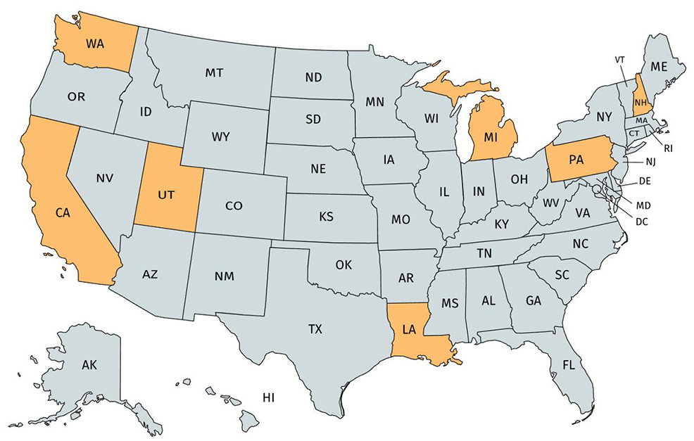
States whose data were used in model development.

Annual Mileage Estimation Models

The utilization models estimate the average annual mileage for different equipment types and classes at a region level based on the data provided by state DOTs. From all explanatory variables that were considered in the modeling process based on the literature review and agency survey findings, eight explanatory variables were found to affect the utilization metrics statistically. These variables are summarized in Table 1. The minimum, mean, and maximum values for each of these parameters and each equipment type are provided in Table 2. The research team developed annual mileage estimation for seven different non-stationary equipment types: dump trucks, pickup trucks, automobiles, vans, sport utility vehicles, truck tractors, and large trucks with a special body.

Table 1.

Definition of Utilization Parameters

Variable		Description
$x_{AM} :$	Annual mileage	The average annual mileage in a region
$x_{FU} :$	Frequency of usage	The average frequency of usage in a region
$x_{PC} :$	Purchase cost ( $\times 10^{- 3})$	The average equipment purchase cost in a region
$x_{DH} :$	Annual downtime hours	The average equipment annual downtime hour in a region
$x_{SMC} :$	Annual scheduled maintenance cost ( $\times 10^{- 3})$	The average equipment annual scheduled maintenance cost in a region
$x_{URC} :$	Annual unscheduled repair cost ( $\times 10^{- 3})$	The average equipment annual unscheduled repair cost in a region
$x_{ISA} :$	In-service age	The average equipment in-service age in a region
$x_{FS} :$	Fleet size	The average fleet size in a region
$x_{C_{i}} :$	Class $i$	1: if the equipment is in class $i$ based on National Association of Fleet Administrators (NAFA) class code (higher value of $i$ is associated with higher weight)

Table 2.

Summary of Utilization Parameters

Utilization parameters	Dump trucks	Pickup trucks	Automobiles	Vans	Sport utility vehicles	Truck tractors	Large trucks with a special body
Annual mileage
Min	1,904	3,396	4,183	847	4,419	736	2,285
Mean	9,166	9,829	9,049	9,546	11,436	10,480	8,943
Max	22,823	22,328	18,704	25,889	20,005	33,559	23,753
Purchase cost
Min	27,585	17,459	18,010	16,651	18,210	39,052	26,052
Mean	79,347	27,311	21,531	29,004	23,711	103,415	56,385
Max	241,832	39,826	25,798	38,509	30,956	225,830	143,475
Annual downtime hours
Min	7	1	6	6	5	16	13
Mean	668	181	127	141	79	77	83
Max	3,155	799	416	609	426	447	633
Annual scheduled maintenance cost
Min	85	93	81	89	104	204	58
Mean	1,731	1,028	428	983	771	1,596	830
Max	17,071	2,770	996	6,271	1,614	4,980	3,090
Annual unscheduled repair cost
Min	249	548	384	322	140	618	1,144
Mean	8,037	2,467	1,373	2,040	2,181	5,771	3,868
Max	80,022	9,295	3,328	8,125	6,731	12,818	8,356
In-service age
Min	2	3	2	3	2	5	3
Mean	10	8	7	10	6	11	10
Max	28	14	12	25	12	25	25
Fleet size
Min	1	2	1	1	1	1	1
Mean	45	79	58	27	45	5	46
Max	320	465	242	234	360	28	303

The collected data were aggregated at the district/region level over all years. Therefore, each data point corresponds to the average of several observations over several years of data and all equipment units with the same NAFA class code in a region. The right-most column of Table 3 shows the sample size before and after aggregation for each fitted model. Aggregation across regions and years was necessary to eliminate the unwanted noise in the collected data. Table 3 also shows fitted models for seven equipment types along with their adjusted R-squared values. Note that the minimum adjusted R-squared value is 0.65, which indicates a good fit. The sample size for all equipment types after aggregation ranges from 31 to 98 observations, which is enough to construct prediction models.

Table 3.

Summary of Equipment Utilization Estimation Methods

Equipment type	Utilization estimation model	Adjusted R-squared	Sample size after/before aggregation
Dump trucks	$\begin{matrix} \log (x_{AM}) = 9.321 + 0.238 \log (x_{PC}) - 0.635 \log (x_{ISA}) \\ + 0.129 \log (x_{URC} / x_{SMC}) - 0.503 (x_{C_{5}} + x_{C_{6}} + x_{C_{7}}) \end{matrix}$	0.65	98/15,338
Pickup trucks	$\begin{matrix} \log (x_{AM}) = 7.081 + 0.461 \log (x_{PC}) - 0.153 {(x_{ISA})}^{0.5} \\ + 0.275 \log (x_{URC} / x_{SMC}) + 0.237 \log (x_{DH}) \\ - 0.024 {(x_{FS})}^{0.5} - 0.049 x_{C_{2}} - 0.144 x_{C_{3}} \\ - 0.464 x_{C_{4}} \end{matrix}$	0.89	78/15,334
Automobiles	$\log (x_{AM}) = 9.119 + 0.256 x_{SMC} + 0.0781 \log (x_{DH}) - 0.147 \log (x_{FS})$	0.74	32/4,327
Vans	$\begin{matrix} \log (x_{AM}) = 9.256 - 0.111 x_{ISA} + 0.103 \log (x_{URC} / x_{SMC}) \\ + 0.188 \log (x_{DH}) - 0.002 x_{FS} + 0.289 (x_{C_{5}} + x_{C_{6}}) \end{matrix}$	0.80	55/3,384
Sport utility vehicles	$\log (x_{AM}) = 10.222 - 0.461 \log (x_{ISA}) + 0.248 \log (x_{SMC}) - 0.002 x_{FS}$	0.81	37/2,956
Truck tractors	$\begin{matrix} \log (x_{AM}) = 10.014 - 0.004 {(x_{PC} \times 10^{- 1})}^{2} \\ - 0.810 \log (x_{ISA}) + 0.061 x_{URC} + 1.064 x_{C_{3}} \end{matrix}$	0.77	31/483
Large trucks with a special body	$\begin{matrix} \log (x_{AM}) = 9.712 - 0.080 x_{ISA} + 0.158 \log (x_{URC}) \\ - 9.27 {(x_{FS} \times 10^{- 3})}^{2} + 0.284 x_{C_{2}} - 0.296 x_{C_{5}} \\ - 1.032 x_{C_{8}} - 0.278 x_{C_{11}} \end{matrix}$	0.86	76/12,690

All fitted models predict the logarithmic function of annual mileage for different equipment types based on several explanatory variables. Note that all reported coefficients are statistically significant at a 95% confidence level. Moreover, the majority of explanatory variables have the same signs in different models, indicating that they influence the annual mileage of different equipment types in the same way. The in-service age of dump trucks, pickup trucks, vans, sport utility vehicles, truck tractors, and large trucks with a special body has a negative association with their corresponding average annual mileage in a region. The negative association shows that DOTs tend to use the older equipment less frequently, since newer equipment assets are more reliable, cost-effective, and convenient to use. In addition, newer equipment fleets are more efficient in fuel consumption. Moreover, the utilization of dump trucks, sport utility vehicles, and truck tractors has a logarithmic relationship with in-service age. In addition, the utilization of pickup trucks has a relationship with square root of in-service age. These relationships mean that the effect of in-service age on the utilization reduction of newer equipment is higher than for older equipment. In other words, while the utilization of equipment reduces as it ages, the rate of reduction decreases as well.

The average scheduled maintenance costs have a positive association with the average annual mileage of automobiles and sport utility vehicles. This indicates that well-maintained equipment assets operate with higher efficiency and, as a result, are utilized more. The average unscheduled repair cost factor is also positively associated with the average annual mileage of truck tractors and large trucks with a special body. This would be explained by the higher chance of breakdown when the equipment is used more frequently. The models also show that the ratio of average unscheduled repair cost to the average scheduled maintenance costs has a positive association with the utilization of dump trucks, pickup trucks, and vans. As a result, the over-usage of equipment fleets may lead to a significant increase in average repair costs in comparison with maintenance costs. In addition, it was observed that the purchase cost of truck tractors had a negative association with usage. This could be attributed to assigning expensive truck tractors mostly to specialty tasks rather than everyday tasks because of their higher price tag, more maintenance costs, and their additional capabilities.

Based on the results of the models, the fleet size in a region has a negative association with the average fleet utilization of pickup trucks, automobiles, vans, sport utility vehicles, and large trucks with a special body. This is explained by the underutilization of equipment assets in a region where the demand is distributed among a greater number of equipment assets. Models also show that the average downtime hours have positive associations with the average annual mileage of pickup trucks, automobiles, and vans. When equipment assets are utilized more, the chance of breakdown increases. Therefore, downtime hours will be increased.

The average purchase costs of dump trucks and pickup trucks are positively associated with their corresponding average annual mileage. This means that more expensive equipment is used more frequently. However, the purchase cost has a negative association with the utilization of truck tractors. Truck tractors are not utilized extensively by state DOTs, as indicated by their low sample size. It is hypothesized that more expensive truck tractors become more specialized and as such utilized less by state DOTs. Finally, the models show that the NAFA class codes have a significant association with the utilization of dump trucks, pickup trucks, and large trucks with special bodies. Particularly, the heavier equipment assets are utilized less in state DOTs.

For the sake of illustration, Table 4 provides detailed information on estimated parameters of the developed utilization model for dump trucks, where all coefficients are statistically significant. Purchase cost, in-service age, and the ratio of annual unscheduled repair cost to scheduled maintenance cost are present in the model with a logarithmic functional form. The main reason is that an increase in these variables at lower values yields a more significant change in the annual mileage compared with that at higher values. For instance, an increase in the age of a newer equipment unit reduced annual mileage much more than the same increase in the age of an older equipment unit.

Table 4.

Utilization Model for Dump Trucks

Y: log (annual mileage)
Term	Estimate	Std error	Statistic	p-value
Intercept	9.321	1.266	6.064	0.000
log (Purchase Cost)	0.238	0.110	2.160	0.034
log (In-Service Age)	−0.635	0.085	−7.494	0.000
log (Annual Unscheduled Repair Cost/Scheduled Main Cost)	0.129	0.027	4.820	0.000
Class 5 & 6 & 7 (>19,500 GWV)	−0.503	0.100	−5.048	0.000

Validation of Annual Mileage Estimation Models

Figure 2 shows the histograms for residuals of the utilization estimation models. The residuals are defined as the difference between the estimated and observed annual mileage. Therefore, they were expected to have an average value of zero and be normally distributed. All histograms follow a bell-shaped curve around the value of zero and seem to follow a normal distribution. The graph shows that models for truck tractors, vans, large trucks with special body, sport utility vehicles, dump trucks, automobiles, and pickup trucks have the highest to lowest standard deviations in order. Lower standard deviation will be associated with more accurate prediction performance.

Figure 2.

Histograms of residuals of the utilization estimation models: (a) dump trucks, (b) pickup trucks, (c) automobiles, (d) vans, (e) sport utility vehicles, (f) truck tractors, and (g) large trucks with special body.

The quantile-quantile (Q-Q) plots in Figure 3 graphically confirm that the residuals are normally distributed. The Q-Q plot displays the residuals against normally distributed values and helps assess if the residuals plausibly came from a normal distribution. The residuals are almost normally distributed as they lie on a straight line between the upper and lower 95% confidence intervals.

Figure 3.

Quantile-quantile plots: (a) dump trucks, (b) pickup trucks, (c) automobiles, (d) vans, (e) sport utility vehicles, (f) truck tractors, and (g) large trucks with special body.

Figure 4 shows the logarithmic values of the predicted annual mileage versus its observed values for all equipment types. As can be seen in the figure, the fitted lines to the predicted versus observed points have slopes of almost one, and the observations are distributed close to the line. The findings confirm that the annual mileage prediction models work accurately.

Figure 4.

Plots of predicted versus observed values: () dump trucks, (b) pickup trucks, (c) automobiles, (d) vans, (e) sport utility vehicles, (f) truck tractors, and (g) large trucks with special body.

In addition to comparing the estimated and observed annual mileage values, Table 5 shows the adjusted R-squared values for each fitted estimation model. The adjusted R-squared values ranged from 0.65 to 0.89 and confirm that the models accurately estimate the annual mileage for equipment types that have available data. Moreover, the research team performed several statistical tests to ensure that the assumptions of regression analyses are met. An alpha value of 0.05, corresponding to a 95% significance level, was used. Therefore, any P-value that is greater than 0.05 indicates that the null hypothesis cannot be rejected: it cannot be rejected that the assumption was met. Therefore, it is desired to see high P-values especially greater than 0.05. The Shapiro-Wilk test, Durbin–Watson statistic, and Breusch–Pagan test were used to ensure the satisfaction of assumptions. The results are shown in Table 5. The null hypothesis for the Shapiro-Wilk test represents that the model residuals are normally distributed. A high P-value indicates that the null hypothesis is not rejected: the residuals are distributed normally. All equipment estimation models show high P-values, indicating that the residuals are normally distributed, which confirms the findings in Figures 2 and 3.

Table 5.

Validation Results of the Utilization Estimation Models

Equipment type	Adjusted R-squared	Sample size	Shapiro test P-value	Durbin–Watson test P-value	Breusch–Pagan test P-value
Dump trucks	0.65	98	0.455	0.08	0.056
Pickup trucks	0.89	78	0.432	0.634	0.717
Automobiles	0.74	32	0.419	0.636	0.568
Vans	0.80	55	0.752	0.164	0.388
Sport utility vehicles	0.81	37	0.947	0.064	0.367
Truck tractors	0.77	31	0.764	0.154	0.356
Large trucks with special body	0.86	76	0.367	0.744	0.846

The null hypothesis for the Durbin–Watson test indicates that the linear regression residuals are uncorrelated. Therefore, a high P-value confirms that there is no autocorrelation between residuals in the estimation models. Assuming a 95% confidence interval, the Durbin–Watson test does not reject the null hypothesis for any model.

The homoskedasticity assumption indicates that the variance is constant for all residuals. The result of the Breusch–Pagan test confirms the null hypothesis that there is no heteroskedasticity in the residuals of the fitted models. Assuming a 95% confidence interval, all estimation models provide homoscedastic residuals with high P-values.

Table 6 shows 12 observations for five equipment types in different states and regions. Each observation is an average of several assets in a region and a year. The values of explanatory variables and the corresponding observed usage for different classes of dump trucks, pickup trucks, automobiles, vans, and sport utility vehicles are also provided. The annual mileage for each observation is predicted using the equation provided in Table 3. The comparison between the actual and the predicted usage for each observation confirms that the utilization models provide predictions with enough accuracy. Table 6 shows the prediction error for these observations. The maximum error is 8.6% and the minimum error is 0.78%.

Table 6.

Actual and Predicted Utilizations for Seven Observations

Asset type	State	Region	Avg purchase cost ($)	Avg in-service age	Avg unscheduled repair cost ($)	Avg scheduled maintenance cost ($)	Avg down time hours	Fleet size	Class	Actual usage (mile)	Predicted usage (mile)	Prediction error (%)
Dump truck	MI	Bay	120,384	10	36,810	16,307	1,056	32	7	6,033	5,795	3.94
		Metro	103,860	14	9,624	3,083	1,349	19	7	3,955	4,221	−6.73
		North	129,678	9	15,889	5,239	1,042	16	7	6,742	6,546	2.91
Pickup truck	UT	Region 1	20,133	7	819	112	5	71	2	6,415	6,146	4.19
		Region 4	21,035	7	916	154	6	127	2	5,826	5,908	−1.41
Auto	LA	District 2	15,528	10	402	201	122	27	1	8,706	8,620	0.99
		District 4	15,066	10	503	261	116	15	1	10,045	9,509	5.34
Van	NH	District 1	21,716	4	2,750	1,604	488	20	2	23,160	22,808	1.52
		District 4	24,092	3	2,074	1,010	424	12	2	25,086	24,233	3.40
Sport utility vehicle	PA	District 1	19,197	3	4,153	1,492	129	11	1	18,101	17,479	3.44
		District 3	20,223	2	3,946	1,542	89	13	1	20,020	21,761	−8.70
		District 9	19,536	3	3,929	1,506	95	19	1	18,850	18,703	0.78

Annual Operating Cost Estimation Models

In addition to the utilization estimation models, the research team developed models to estimate the total operating cost of the same seven non-stationary equipment types. The annual operating cost is defined as the summation of annual fuel cost, unscheduled repair cost, and scheduled maintenance cost. The annual operating cost is the dependent variable in the regression analysis. The independent variables include:

-annual mileage,

-annual downtime hour,

-in-service age,

-fleet size in a region, and

-class of equipment, and

Table 7 shows the summary of the fitted cost functions. The variables are explained in Table 1. Let $x_{OC}$ represent the annual operating cost (the summation of annual fuel cost, annual unscheduled repair cost, and annual scheduled maintenance cost in the unit of $1,000). Moreover, Table 7 shows the R-squared associated with each fitted model and the sample size before and after the aggregation of data.

Table 7.

Summary of Equipment Operating Cost Estimation Models

Equipment type	Operating cost estimation model	Adjusted R-squared	Sample size after/before aggregation
Dump trucks	$\begin{matrix} x_{OC} = 12.3 \times 10^{- 12} \times x_{AM} \times {(x_{DH})}^{2} \times {(x_{ISA})}^{2} - 0.027 x_{FS} + \\ 6.262 (x_{C_{1}} + x_{C_{2}} + x_{C_{3}} + x_{C_{4}}) + 1.416 x_{C_{5}} + 1.389 \end{matrix}$ ( $x_{C_{6}} + x_{C_{7}})$	0.59	97/5769
Pickup trucks	$\begin{matrix} x_{OC} = 17.4 \times 10^{- 5} x_{AM} - 18 \times 10^{- 6} x_{FS} \times x_{DH} \\ + 2.719 (x_{C_{1}} + x_{C_{2}}) + 3.442 (x_{C_{3}} + x_{C_{4}}) \end{matrix}$	0.63	72/8721
Automobiles	$\begin{matrix} x_{OC} = 14 \times 10^{- 5} x_{AM} - 3.9 \times 10^{- 3} x_{DH} + 0.699 {(x_{ISA})}^{0.5} \\ - 7.3 \times 10^{- 4} x_{FS} \times {(x_{DH})}^{0.5} \end{matrix}$	0.77	32/1892
Vans	$x_{OC} = 3.6 \times 10^{- 4} x_{AM} - 3.85 \times 10^{- 3} x_{DH} + 0.145 x_{ISA}$	0.69	49/1903
Sport utility vehicles	$\begin{matrix} x_{OC} = 2.4 \times 10^{- 4} x_{AM} - 1.115 \log (x_{DH}) \\ + 2.679 \log (x_{ISA}) - 3.99 \times 10^{- 3} x_{FS} \end{matrix}$	0.81	19/538
Truck tractors	$x_{OC} = 9.2 \times 10^{- 4} x_{AM} - 0.025 x_{DH} + 3.093 x_{C_{2}} + 6.933 x_{C_{3}}$	0.74	26/44
Large trucks with special body	$\begin{matrix} x_{OC} = 3.2 \times 10^{- 4} x_{AM} - 0.229 {(x_{DH})}^{2} + 1.151 \log (x_{ISA}) \\ - 0.053 x_{FS} + 0.020 x_{FS} \times \log (x_{DH}) + 3.696 x_{C_{5}} \\ + 3.006 x_{C_{8}} + 6.582 x_{C_{11}} \end{matrix}$	0.71	45/3585

All coefficients in the models are statistically significant at a 95% confidence level. The average annual mileage of all equipment types is positively associated with their operating costs, as expected. Higher utilization yields to higher fuel costs and higher maintenance and repair costs since the chance of a breakdown increases. Moreover, the fleet size has a negative association with the average operating costs of dump trucks, automobiles, sport utility vehicles, and large trucks with a special body. Possessing numerous equipment assets in a region allows DOTs to maintain their equipment assets at a lower per equipment cost.

The average in-service age of dump trucks, automobiles, vans, sport utility vehicles, and large trucks with a special body has a positive relationship with their corresponding operating costs. This is expected since there is a higher chance of older equipment breaking down more frequently. In addition, older equipment is less efficient in fuel consumption. The average downtime hours of equipment also has a negative association with the operating costs of pickup trucks, automobiles, vans, sport utility vehicles, and large trucks with a special body. This might be explained by not using the equipment after breakdown. Finally, the models show that the class of equipment has a significant impact on the operating cost of dump trucks, pickup trucks, truck tractors, and large trucks with a special body.

The fitted models cannot capture geographical distribution effects on the utilization and operating costs. The dataset used in this study is collected from seven different states across the U.S.A. and further insight would be gained by assessing if the location of equipment has significant impacts on its utilization and the associated costs. Volovski et al. ( 1 ) showed that a random effect model has a good capability to account for the spatial heterogeneity in the dataset, where the variation between observations in different spatial groups is considered. Table 8 shows the new utilization and cost models based on the random intercept to allow the variation based on the state in which an equipment unit is located.

Table 8.

Summary of Random Effect Models for Utilization and Cost Estimation

Equipment type	Model	Random effects on state
		Intercept std dev.	Residual
Utilization estimation models
Dump trucks	$\begin{matrix} \log (x_{AM}) = 10.010 + 0.0063 x_{PC} - 0.697 \log (x_{ISA}) \\ + 0.237 \log (x_{URC}) - 0.073 \log (x_{SMC}) \\ - 0.334 (x_{C_{5}} + x_{C_{6}} + x_{C_{7}}) \end{matrix}$	0.166	0.354
Pickup trucks	$\begin{matrix} \log (x_{AM}) = 4.398 + 0.413 \log (x_{PC}) - 0.158 {(x_{ISA})}^{0.5} \\ + 0.279 \log (x_{URC} / x_{SMC}) + 0.231 \log (x_{DH}) \\ - 0.023 {(x_{FS})}^{0.5} - 0.456 x_{C_{4}} \end{matrix}$	0.082	0.156
Automobiles	$\begin{matrix} \log (x_{AM}) = 8.463 + 0.125 \log (x_{SMC}) \\ + 0.074 \log (x_{DH}) - 0.143 \log (x_{FS}) \end{matrix}$	0.000005	0.219
Vans	$\log (x_{AM}) = 9.324 - 0.1041 x_{ISA} + 0.181 \log (x_{DH}) - 0.002 x_{FS}$	0.00001	0.318
Sport utility vehicles	$\log (x_{AM}) = 8.237 - 0.257 \log (x_{ISA}) + 0.221 \log (x_{SMC})$	0.285	0.131
Truck tractors	$\begin{matrix} \log (x_{AM}) = 9.741700 - 0.00001 {(x_{PC} \times 10^{- 1})}^{2} \\ - 0.603 \log (x_{ISA}) + 1.005 x_{C_{3}} \end{matrix}$	0.356	0.392
Large trucks with a special body	$\begin{matrix} \log (x_{AM}) = 8.045 - 0.081 x_{ISA} + 0.226 \log (x_{URC}) \\ - 0.000007 {(x_{FS})}^{2} + 0.273 x_{C_{2}} - 0.292 x_{C_{5}} \\ - 0.958 x_{C_{8}} - 0.428 x_{C_{11}} \end{matrix}$	0.173	0.201
Operating cost estimation model
Dump trucks	$\begin{matrix} x_{OC} = 10.1 \times 10^{- 10} \times x_{AM} \times x_{DH} \times x_{ISA} \\ - 0.680 \log (x_{FS}) + 6.615 (x_{C_{1}} + x_{C_{2}} + x_{C_{3}} + x_{C_{4}}) + 8.967 x_{C_{5}} \\ + 11.259 \end{matrix}$ ( $x_{C_{6}} + x_{C_{7}})$	4.684	4.983
Pickup trucks	$\begin{matrix} x_{OC} = 9.2 \times 10^{- 5} x_{AM} \times \log (x_{ISA}) - 0.100 \log (x_{DH}) \\ + 2.945 (x_{C_{1}} + x_{C_{2}}) + 3.486 (x_{C_{3}} + x_{C_{4}}) \end{matrix}$	0.490	0.850
Automobiles	$\begin{matrix} x_{OC} = 7.1 \times 10^{- 5} x_{AM} + 0.282 \log (x_{DH}) + 0.216 \log (x_{ISA}) \\ - 2.5 \times 10^{- 5} x_{FS} \times x_{DH} \end{matrix}$	0.985	0.358
Vans	$x_{OC} = 2.4 \times 10^{- 4} x_{AM} + 0.764 \log (x_{DH}) + 0.951 \log (x_{ISA})$	3.677	0.874
Sport utility vehicles	$\begin{matrix} x_{OC} = 1.7 \times 10^{- 4} x_{AM} - 0.347 \log (x_{DH}) \\ + 0.924 \log (x_{ISA}) + 0.001 x_{FS} \end{matrix}$	1.788	0.440
Truck tractors	$\begin{matrix} x_{OC} = 1.2 \times 10^{- 3} x_{AM} - 0.025 x_{DH} - 2.697 x_{C_{2}} \\ + 0.965 x_{C_{3}} - 0.040 x_{FS} \times \log (x_{DH}) \end{matrix}$	6.524	2.996
Large trucks with special body	$\begin{matrix} x_{OC} = 3.4 \times 10^{- 4} x_{AM} + 0.541 \log (x_{DH}) + 0.386 \log (x_{ISA}) \\ + 0.018 x_{FS} + 0.020 x_{FS} + 0.339 x_{C_{5}} \\ + 0.395 x_{C_{8}} + 2.831 x_{C_{11}} \end{matrix}$	1.951	1.308

Furthermore, Table 9 shows the comparison between the fixed effect and random effect models using the ANOVA test. The comparison shows that geographical distribution has a significant impact on the utilization estimation of dump trucks, automobiles, sport utility vehicles, truck tractors, and large trucks with a special body. In addition, comparison of the cost estimation models shows that the geographical distribution significantly affects the costs associated with all equipment types.

Table 9.

Comparison of Fixed Effect and Random Effect Models

Equipment type	Model	AIC	BIC	logLik	L.Ratio	P-value
Utilization estimation models
Dump truck	Fixed effect	121.523	137.389	−54.761	na	na
	Random effect	118.426	136.937	−52.213	5.096	0.024
Pickup truck	Fixed effect	2.539	23.144	8.730	na	na
	Random effect	2.226	24.891	9.887	2.314	0.1282
Automobile	Fixed effect	29.5662	35.02141	−9.783101	na	na
	Random effect	21.24266	27.78891	−4.621329	10.32354	0.0013
Van	Fixed effect	71.963	85.621	−28.981	na	na
	Random effect	68.942	80.876	−28.471	1.021	0.3123
Sport utility vehicles	Fixed effect	21.324	27.804	−5.662	na	na
	Random effect	5.048	12.823	3.476	18.277	<.0001
Truck tractors	Fixed effect	121.671	129.220	−54.836	na	na
	Random effect	116.631	125.438	−51.316	7.040	0.008
Large Trucks with a special body	Fixed effect	52.655	71.653	−17.328	na	na
	Random effect	46.367	67.475	−13.183	8.289	0.004
Operating cost estimation models
Dump truck	Fixed effect	1953.584	1968.715	−970.792	na	na
	Random effect	1905.380	1923.033	−945.690	50.2041	<.0001
Pickup truck	Fixed effect	1134.672	1145.620	−562.335	na	na
	Random effect	1129.638	1142.776	−558.818	7.033	0.008
Automobile	Fixed effect	284.416	287.612	−137.208	na	na
	Random effect	270.885	274.719	−129.442	15.531	0.0001
Van	Fixed effect	812.675	819.902	−402.337	na	na
	Random effect	792.134	801.167	−391.067	22.540	<0.0001
Sport utility vehicles	Fixed effect	257.934	260.759	−123.967	na	na
	Random effect	250.903	254.293	−119.451	9.030	0.0027
Truck tractors	Fixed effect	365.267	369.130	−177.633	na	na
	Random effect	348.130	352.765	−168.065	19.137	<0.0001
Large trucks with special body	Fixed effect	692.070	707.9054	−336.0351	na	na
	Random effect	689.238	706.656	−333.619	4.832	0.0279

Note: AIC = Akaike information criterion; BIC = Bayesian information criterion; L.Ratio = Likelihood ratio; na = not applicable.

In an additional experiment, the fixed effect models were adjusted to have a different intercept for each state. Table 10 shows the comparison between the fixed effect and random effect models after this change. We can see that there is no statistically significant difference between the fixed effect models with separate intercepts for each state and the random effect models. In other words, having several intercepts for each state improves the predictability of the fixed effect model by taking into account the geographical distribution.

Table 10.

Comparison of Fixed Effect Model with Several Intercepts for Each State and Random Effect Models

Equipment type	Model	AIC	BIC	logLik	L.Ratio	P-value
Utilization estimation models
Dump truck	Fixed effect	115.856	134.007	−51.428	na	na
	Random effect	118.426	136.937	−52.213	8.24	0.121
Pickup truck	Fixed effect	2.17	30.017	10.91	na	na
	Random effect	6.041	28.706	9.887	9.869	0.089
Automobile	Fixed effect	18.401	25.956	−1.200	na	na
	Random effect	21.242	27.788	−4.621	6.841	0.062
Van	Fixed effect	75.231	94.149	−27.615	na	na
	Random effect	68.942	80.876	−28.471	1.710	0.788
Sport utility vehicles	Fixed effect	6.182	15.606	4.908	na	na
	Random effect	5.048	12.823	3.476	2.865	0.238
Truck tractors	Fixed effect	74.233	83.657	−29.11	na	na
	Random effect	75.184	83.991	−30.592	2.951	0.085
Large trucks with a special body	Fixed effect	50.287	75.012	−13.143	na	na
	Random effect	46.367	67.475	−13.183	0.0791	0.961
Operating cost estimation models
Dump truck	Fixed effect	642.985	667.758	−311.492	na	na
	Random effect	634.353	652.005	−310.176	2.631	0.451
Pickup truck	Fixed effect	214.781	233.925	−99.390	na	na
	Random effect	217.813	230.951	−100.906	9.032	0.228
Automobile	Fixed effect	79.686	82.409	−30.843	na	na
	Random effect	77.467	81.302	−32.733	3.781	0.286
Van	Fixed effect	179.985	193.694	−81.992	na	na
	Random effect	170.436	179.469	−80.218	3.548	0.314
Sport utility vehicles	Fixed effect	6.1820	15.606	4.908	na	na
	Random effect	5.047	12.822	3.476	2.865	0.238
Truck tractors	Fixed effect	134.166	138.414	−61.083	na	na
	Random effect	127.082	131.717	−59.541	9.322	0.406
Large trucks with special body	Fixed effect	190.170	208.486	−83.085	na	na
	Random effect	191.879	209.298	−84.939	3.709	0.154

Note: AIC = Akaike information criterion; BIC = Bayesian information criterion; L.Ratio = Likelihood ratio; na = not applicable.

Conclusion

Highway agencies use a variety of processes for measurement and management of utilization of their equipment fleets. However, there are no widely accepted processes for estimating utilization of fleet equipment. Therefore, the utilization estimation models in this study provide the capability to manage certain fleet equipment types and classes. This research adopted the NAFA classification system to provide a standardized definition that can be used at all state DOTs in the U.S.A. In addition, factors that are important to the estimation of utilization of fleet equipment are described.

This paper presents the development of two sets of models to estimate annual mileage and annual operational cost of seven non-stationary equipment types as a function of several contributing factors (e.g., fuel cost, downtime hours, age, class, and fleet size). The research team reviewed the literature and identified annual mileage as the most important utilization metric. The research team performed a national data collection exercise and finally utilized data from seven state DOTs. The research team found the logarithmic function to represent the relationship between annual mileage and the explanatory variables more appropriately than other forms.

The adjusted R-square of the utilization estimation models ranged from 0.65 to 0.89 which indicates a good fit. The annual operational cost models had adjusted R-squares ranging between 0.59 and 0.81, which also indicates a good fit. Both models were validated and it is observed that both models satisfy the assumptions of linear regression. The models developed in this paper are intended to be used by state DOTs or other public agencies that operate highway maintenance equipment. While state DOTs could use their own data to fit new models that represent their state more accurately, the models developed in this research can be used directly.

The results show that the average in-service age, annual downtime hours, annual scheduled maintenance costs, annual unscheduled repair costs, fleet size in a region, and equipment class have a significant association with the average annual mileage of different equipment types. Higher in-service age, annual downtime hours, and maintenance and repair costs are most associated with higher utilization levels. On the other hand, a larger fleet size in a region is associated with lower utilization of equipment. In addition, equipment with higher weight tends to be used less frequently.

The estimation models showed that the average annual mileage, in-service age, annual downtime hours, fleet size in a region, and equipment class have significant associations with the operating cost of equipment. Particularly, higher annual mileage and in-service age yield higher operating costs. On the other hand, higher values of fleet size and annual downtime hours are associated with lower operating costs.

This research constructed the prediction models based on data received from seven states. The developed models could become more representative of the U.S.A. overall if data from more states in different regions were included in the research. The research did not include a calibration process; however, standard calibration methods can be applied to use the presented models in different states. The literature review and agency survey findings indicated that seasonality, climate, and ownership are among important factors that are expected to contribute to equipment utilization and management. This research could not include them in the prediction models because of lack of data. Further research is needed to incorporate these contributing factors in utilization prediction models and study their impacts on equipment utilization management.

Footnotes

Acknowledgements

The authors are grateful for the financial support of the National Highway Cooperative Research Program (NCHRP 13-05), which sponsored this research. This work represents a portion of a larger project, “Guide for Utilization Measurement and Management of Fleet Equipment.” The authors would like to thank the NCHRP panel and Senior Program Officer, Dr Amir Hanna, for providing invaluable feedback and guidance, and other researchers that contributed to the completion of this research: Dr Wei Fan, Mr Miao Yu, Dr Xianming She, Mr Mike Moser, and Mr Shaowei Wang.

Author Contributions

The authors confirm contribution to the paper as follows: study conception and design: A. Hajbabaie and L. Hajibabai; data collection: M. Tajalli and L. Hajibabai; analysis and interpretation of results: M. Tajalli, A. Mirheli, A. Hajbabaie, L. Hajibabai; draft manuscript preparation: M. Tajalli, A. Hajbabaie, and L. Hajibabai. All authors reviewed the results and approved the final version of the manuscript.

Declaration of Conflicting Interests

The author(s) declared no potential conflicts of interest with respect to the research, authorship, and/or publication of this article.

Funding

The author(s) declared that they received the following financial support for the research, authorship, and/or publication of this article: the National Highway Cooperative Research Program (NCHRP 13-05) sponsored this research.

ORCID iDs

Amir Mirheli

Ali Hajbabaie

Leila Hajibabai

The opinions and conclusions stated in this paper strictly reflect those of the authors and not of NCHRP or its constituent members. This paper does not constitute a standard, specification, or regulation.

References

Volovski

Murillo-Hoyos

Saeed

T. U.

Labi

Estimation of Routine Maintenance Expenditures for Highway Pavement Segments: Accounting for Heterogeneity Using Random-Effects Models. Journal of Transportation Engineering, Part A: Systems, Vol. 143, 2017, p. 4017006.

Gransberg

D. D.

O’Connor

E. P.

Major Equipment Life-Cycle Cost Analysis. Report No. MN/RC 2015-16. Minnesota Department of Transportation, St Paul, 2015.

Mirheli

Tajalli

Mohebifard

Hajibabai

Hajbabaie

Utilization Management of Highway Operations Equipment. Transportation Research Record: Journal of the Transportation Research Board, 2020. 2674: 202–215.

Hajibabai

Hajbabaie

Tajalli

Mirheli

Fan

NCHRP Research Report 957. Utilization Measurement and Management of Fleet Equipment. NCHRP Project 13-05. Transportation Research Board of the National Academies, Washington, D.C., 2021. https://www.nap.edu/catalog/26067.

Optimize Your Assets – Fast and Easy. BEB Industrial Asset Management. http://www.bebsoft.com/index.html. Accessed September 10, 2019.

Imhoff

White

Master Data Management: Creating a Single View of the Business. Powell Media, LLC, Intelligent Solutions and BI Research, 2006. https://www.cnblogs.com/spidertan/archive/2007/06/21/791414.html.

Mercury Associates, Inc. NASA Official Fleet Management Handbook. National Aeronautics and Space Administration, Washington, D.C., 2005.

Woldemariam

Murillo-Hoyos

Labi

Estimating Annual Maintenance Expenditures for Infrastructure: Artificial Neural Network Approach. Journal of Infrastructure Systems, Vol. 22, 2016, p. 4015025.

Yost

Ohio Department of Transportation Performance Audit. Ohio Department of Transportation, 2013.

10.

Management Partners Incorporated. City of San Bernardino Fleet Services Assessment and Utilization Analysis. 2007. https://docplayer.net/18710179-Appendix-a-city-of-san-bernardino-fleet-services-assessment-and-utilization-analysis-february-2007.html.

11.

Minnesota Department of Transportation. Minnesota Statewide Highway Systems Operation Plan. Minnesota Department of Transportation, 2012.

12.

Osterstock

Kidd

Eliason

Hicken

A Performance Audit of the Division of Fleet Operations. Utah. Legislature. Office of the Legislative Auditor General, 2005.

13.

CTC & Associates LLC. Fleet Equipment Asset Management Performance Measures. Caltrans Division of Research and Innovation, 2012. https://dot.ca.gov/-/media/dot-media/programs/research-innovation-system-information/documents/preliminary-investigations/fleet-equipment-performance-measures-pi-a11y.pdf.

14.

Kader

Ramani

T. L.

Johnson

J. D.

Speigelman

Zietsman

Jacobs

Fleet Equipment Performance Measurement Preventive Maintenance Model: Final Report. Report No. 0-6626-1. Texas A&M Transportation Institute, College Station, 2014.

15.

Weissmann

A. J.

Gona

Texas Equipment Replacement Model (TERM) Software Manual. Research Report 0-4941-3. University of Texas, San Antonio, 2003.

16.

Fan

Haile

Chavez

Radley

Sorbet

Eifert

Machemehl

Gemar

Murshed

Equipment Replacement/Retention Decision Making. Report No. 0-6693-1. Texas Department of Transportation, Austin, 2015.

17.

White

J. F.

SCDOT Vehicle and Equipment Management: A Certified Public Manager Research Project. South Carolina State Documents Depository, 2005.

18.

Johnson

P. D.

Principles of Controlled Maintenance Management. Fairmont Press, Lilburn, GA, 2002.

19.

Lee

W.-S.

Huang

A. Y.

Chang

Y.-Y.

Cheng

C.-M.

Analysis of Decision Making Factors for Equity Investment by DEMATEL and Analytic Network Process. Expert Systems with Applications, Vol. 38, 2011, pp. 8375–8383.

20.

Vujanović

Momčilović

Bojović

Papić

Evaluation of Vehicle Fleet Maintenance Management Indicators by Application of DEMATEL and ANP. Expert Systems with Applications, Vol. 39, 2012, pp. 10552–10563.

21.

Said

Nicoletti

Perez-Hernandez

Utilizing Telematics Data to Support Effective Equipment Fleet-Management Decisions: Utilization Rate and Hazard Functions. Journal of Computing in Civil Engineering, Vol. 30, 2014, p. 4014122.

22.

Roy

Windover

Idle Reduction Assessment for the New York State Department of Transportation Region 4 Fleet. Report No. C-13-01. New York State Department of Transportation, Albany, 2015.

23.

Kargul

Glaese

Kessler

Günthner

W. A.

Heavy Equipment Demand Prediction with Support Vector Machine Regression Towards a Strategic Equipment Management. International Journal of Structural and Civil Engineering Research, Vol. 6, No. 2, 2017, pp. 137–143.

24.

Rohani

Abbaspour-Fard

M. H.

Abdolahpour

Prediction of Tractor Repair and Maintenance Costs Using Artificial Neural Network. Expert Systems with Applications, Vol. 38, 2011, pp. 8999–9007.