



Abstract
The geography of horizontal roadway curves is critical to various disciplines, especially to transportation safety, because of their strong correlation with traffic crashes. Remarkably, conventional geographic information system (GIS) roadway centerlines, while fundamental and ubiquitous in current geospatial databases, do not include curve inventories. This study presents an improved method for automatic horizontal curve identification using GIS roadway centerline networks as the data source. Analyzing each vertex of the network geometry, this method identifies the curves by detecting deflections from straight lines using a vertex deflection angle threshold. Different from literature that uses a static threshold, this method develops and applies a dynamic threshold by considering two variables—the roadway speed and the centerline vertex density. The method is capable of self-adjusting using k-means clustering to compensate for uneven centerline digitization. The method can also detect spiral transitions and can handle the complexities of street networks represented using dual centerlines. The testing and validation of the method were performed on a large dataset by applying a combination of goodness of fit metric and visual inspection. The results show that this method improves curve identification accuracy and can provide broader applicability for curve identification using GIS centerlines of various representations and digitization quality in large geographic areas.
Geographic information systems (GIS) roadway centerlines are a staple of any geospatial database, in particular those in the transportation area. The location and attributes of horizontal curves in any transportation GIS roadway centerline network are critical for various applications such as transportation safety or to guide vehicle navigation. Roadway curves are one of the major safety hazards in United States with more than one-quarter of highway traffic crash fatalities occurring on them ( 1 , 2 ). Based on historical statistics, horizontal curve alignments have crash rates three times higher than other types of roadway, and much higher crash rates than tangent sections on the same road ( 3 – 5 ). Furthermore, the emergence of autonomous vehicles has increased the demand for accurate GIS street basemaps to support navigation. Knowledge of the location of horizontal curves and their attributes such as radius, length, or a spiral transition in such basemaps can serve as auxiliary information that can proactively inform and assist safe navigation of autonomous vehicles.
Problem Statement
Despite their importance, the issue with curves is at a more basic level; the spatial locations of curves and their attributes are typically not readily available in GIS roadway centerline databases as an identified feature. Most GIS street networks do not include clear demarcation of curve geometries and their attributes despite the need. The Federal Highway Administration (FHWA) requires certain horizontal curve data to address safety concerns. They are defined in the Model Inventory of Roadway Elements (MIRE), a recommended listing of roadway inventory and traffic data elements critical to safety management ( 6 ). In addition to location, the required information for horizontal curves includes curve type, radius, length, and the transition type to name a few. Currently, most agencies obtain roadway curve information either through manual work or semi-automated processes, which are very time-consuming, especially when the size of the roadway network is large. Therefore, an automated procedure is necessary to find the location of curves and calculate their attributes on a GIS roadway network.
Study Objective
The aim of this study was automatic detection and extraction of curves and their characteristics using GIS roadway centerlines as the data source. The study, drawing on existing methods in the literature, developed and implemented an improved method that reflects the need to determine curves in large complex GIS street basemaps for large areas, and considering additional variables not previously used in literature, such as roadway speed and roadway centerline vertex density. The study used Florida’s All Roads GIS Basemap as the data source.
Literature Review
Knowledge of the locations and characteristics of horizontal curves can help transportation agencies locate high-risk segments, apply countermeasures, and improve warning systems. To support these needs, a great deal of research has been conducted in quantifying the factors that affect safety performance related to curve elements, such as curve radius, curve length, degree of curvature, and tangent length. Previous literature ( 7 – 11 ) has examined crash prediction models for curves and has summarized the factors that influence horizontal curve safety. There exists a positive correlation between curve length and crashes, and a negative correlation between curve radius and crashes. Most such research has utilized curve samples based on existing datasets, that is, the curve geometry data from the Highway Safety Information System (HSIS) ( 12 ). However, the curve attributes have not always been available in roadway databases. HSIS does not have the curve attributes for all the participating states. For those states with curve attributes in HSIS, the method of extracting curve information varied from delineating curves manually to developing curve data from construction drawings ( 12 ). The lack of knowledge of the location and the attributes of curves makes it very difficult to study curve safety, screen for high-risk locations, and apply further improvements. Therefore, this raises the question of how to identify curves for large geographic areas in an automated fashion, efficiently, with limited data available.
The literature shows a growing number of studies on automated curve identification using different data sources, such as satellite imagery, GPS data, laser scanning, and GIS. Examples using satellite images ( 13 , 14 ) showed an applicable method to find curves and categorize the curve types. The identification accuracy depended on the imagery resolution and the technique used to distinguish roads from the environment. This method is limited to small geographic areas.
GPS data is also a widely used source for determining roadway curves. GPS-equipped vehicles drive along the target roadways while recording the coordinates at equally spaced time and distance intervals, followed by post-processing of the raw data, and finally the curve characteristics are calculated. This results in high cost and a very long time to collect all the coordinate data for a large number of roadways ( 15 – 17 ).
More recently, light detection and ranging (LiDAR) technology is used as a different approach to finding curves ( 18 ). LiDAR data is collected with the laser scanners mounted on a surface-profiling vehicle which travels along the roadways of interest. This is much more expensive than using GPS equipment and requires more technical expertise. Despite the high tech method, and cost, this method still requires extensive additional manual work.
The traditional GIS roadway centerlines represent another data source used for curve identification. This source is easy to process and has a relatively low cost when considering the large size of linear miles of roadways in large geographic areas. Previous efforts have produced various tools and methods for curve identification using GIS maps. They include the Curve Calculator ( 19 ) from Environmental Systems Research Institute (ESRI), the Curve Extension ( 20 ) from Florida Department of Transportation (FDOT), CurveFinder by Li et al. ( 21 , 22 ), and an improved method by Xu and Wei ( 23 ), and by Wang et al. ( 24 , 25 ). All these tools and methods work on GIS roadway centerlines and calculate the attributes of curves, including curve length and radius. With the first two tools, however, there is still a need to determine the location of the point of curvature (PC) and the point of tangency (PT) on the street network manually. CurveFinder can identify curves automatically and can generate the related attributes by tracking deflection angle changes from vertex to vertex on the dissolved street polylines. Xu and Wei ( 23 ) developed a more complex method than CurveFinder that identifies curves automatically by examining each vertex of the dissolved polylines and turns the deflection angle changes into multiple regression lines whose coefficients represent the curve radii. Wang et al. ( 24 , 25 ) applied a circular regression-based algorithm to extract the PC and the PT. While these methods were successfully evaluated on Interstate segments or national highways, the studies did not indicate any testing on any other roadway types. This could be problematic for other functional roadway classifications which may not have the same high-quality centerline digitization as U.S. Interstates or highways.
GIS roadway centerlines are fundamental and ubiquitous data sources widely used in many application areas. Identifying horizontal curves from GIS centerlines is expected to be a fast and low-cost process, especially when dealing with large geographic areas. Based on the evaluation of the published methods of automatic curve extraction using GIS street data as a source, and considering the characteristics and the size of the source data in this study, it was determined that the CurveFinder was the most suitable source to learn from and improve on. The section below provides additional details focused specifically on this work from the literature.
Definitions and Review of Existing Method
This section presents the curve data elements followed by a brief description of the method, the formulas, and the shortcomings of the CurveFinder as it relates to the aims of this study.
Curve Anatomy
The “anatomy” of the curve geometry, data elements, characteristic points, and curve types is shown in Figure 1 based on the MIRE guideline ( 6 ). Several elements such as PC, PT, PO (point of origin), and radius, to name a few, are used extensively in the computations and application of the curve extraction method.

Model Inventory of Roadway Elements (MIRE) diagrams: (a–d) curve types and (e) components of a simple horizontal curve ( 6 ).
Existing Method: CurveFinder
The CurveFinder method starts by dissolving the segments with the same road name and direction into a single continuous polyline. Next, it scans each polyline at each vertex and by comparing the deflection angle (or bearing angle) of the current vertex to the previous, the CurveFinder determines as “Curve” the collection of segments that have a deflection angle larger than a predetermined threshold (Figure 2a). More information can be found in CurveFinder publications ( 21 , 22 ).

CurveFinder algorithm ( 21 ): (a) bearing angle (deflection angle) as the critical variable in CurveFinder and (b) coordinates needed to calculate curve attributes.
Limitations of CurveFinder
Although the CurveFinder method is feasible to follow, several limitations were encountered when adopting it to the conditions of this study. First, in the present case, the determination of the threshold for the deflection angle required further considerations. This threshold is the only and most essential parameter of the method that affects the results drastically. Using a manual trial and error sensitivity analysis based on ground truth curves, the CurveFinder study had determined 1.25° as the optimal threshold deflection angle that led to the highest identification rate for their GIS source data. However, the drawback of this approach is that the choice of ground truth curves may have a large impact on the optimized threshold deflection angle, leading to different thresholds for different ground truth curves selected, which makes it difficult to provide a constant generalized threshold value that can work for the entire dataset, especially for very large networks.
Second, the formulas used for calculation of curve characteristics assume that the curves are circular and symmetrical. The formula to calculate the curve radius uses PC and PO, as shown in Figure 2b ( 21 ). By analogy, the radius for the same curve can also be calculated using PT and PO. The two radii should be exactly the same in an ideal situation. However, since the digitization of the GIS roadway centerlines does not always result in equally spaced vertices, the two radii may differ. In cases where the GIS network is poorly digitized, the two radii may differ significantly.
Third, although not explicitly stated, according to all the examples published, the CurveFinder basemap uses a single centerline GIS roadway network. When adapting the CurveFinder method for a street basemap with a mixture of single and dual centerlines, some conditions were found that the CurveFinder method had not considered. For example, a centerline may diverge from the path at single-centerline/dual-centerline split and merge points. Obviously, these locations are not curves, but the deflection angle at split/merge points may exceed the deflection angle threshold and incorrectly identify these locations as curves (Figure 3).

Example of split-merge points in a GIS street network with a mixture of single and dual centerlines.
The CurveFinder method, according to the literature, used a portion of the county roads in the selected counties for curve identification. It did not consider the overall variability of the GIS street basemap digitization patterns. The method finally developed for this study, while generally based on the CurveFinder algorithm, is enhanced, and optimized to support a more complex GIS roadway basemap and a more adaptable and dynamic process. The methodology and its implementation are presented below.
Methodology
Source Data
This study used Florida’s All Roads GIS Basemap (based on HERE commercial map). The HERE basemap ( 26 ) was first digitized from the raw data obtained by analysts in vehicles equipped with scanners and GPS, driving around every road in designated areas, along with some help from various sources, such as local governments, utility companies, and other public agencies and commercial mapping agencies. The basemap was further enhanced by utilizing aerial photography and differential GPS for more accuracy. FDOT has added its own Linear Referencing System (LRS) on every HERE road centerline, including local roads.
This basemap contains about 1.8 million links representing roadways by using single centerlines for undivided roads and dual centerlines where a physical divider exists. The basemap contains all classes of roadways including Interstates, state highways, and local roads. The single/dual centerline representation and the inclusion of all classes of roadways adds complexity not previously covered in the curve identification literature.
Input Data Preparation
Curve detection is performed by tracing the entire network vertex by vertex. To support this process, in addition to the GIS street basemap, the method utilizes two additional centerline data layers with a different segmentation structure than the basemap: the route layer and the segment layer (Figure 4).

GIS input data preparation: (a) GIS streets basemap with original segments and nodes, (b) dissolved route layer, and (c) segment layer with vertices.
The route layer consists of long continuous polylines (routes). The route layer was created by applying a GIS dissolve operation to the original segmentation (Figure 4a) based on the route identifier (Roadway_ID) of the LRS. The dissolve using a route identifier can create longer continuous polylines compared with dissolving by street names (in previous studies), given that some roads may simply change names while essentially remaining the same continuous physical roadway. Thus, the dissolved layer contains fewer polylines, which can help accelerate processing speed during the curve detection process. Since the basemap is a mixture of single and dual centerlines, to uniquely identify the left and the right side of dual centerline polylines resulting from the dissolve, an additional identifier (Line_ID) was added for each dissolved polyline. Finally, a route layer based on the dissolved polylines was created using the new Line_ID as the route identifier to uniquely identify each individual polyline (Figure 4b). This route layer constitutes the first input for curve identification procedure.
The second additional input layer, referenced as the segment layer, consists of segments created by splitting the continuous polylines (the route layer) at each vertex (Figure 4c). This layer represents the finest segmentation possible of the GIS street basemap. A new identifier was added to each segment (Sequence_ID), whose values increase incrementally along each route and provide the route tracing direction during the curve detection procedure.
The last step of the data preparation involved creating a special attribute to mark the single and dual centerline split-merge points for the purpose of excluding them during the curve detection procedure (see related discussion below Limitations of CurveFinder). Likewise, the next vertex up each leg of the dual centerline roadway was specially marked for the same purpose. This ensured that when analyzing each vertex during the tracing process, the vertices marked as “split-merge” were skipped, thus avoiding misidentification of these locations as curves (Figure 3).
Curve Identification Algorithm
Figure 5 presents a detailed flowchart of the algorithm developed to identify the curves on the GIS street basemap. The summary of the algorithm is as follows: the algorithm traces vertices along each route while examining the corresponding segments in the segment file. During tracing, the algorithm analyzes the deflection angle between each pair of consecutive segments and compares it with the deflection angle threshold value. When the deflection angle exceeds the threshold, the curve begins. When the angles of deflection of subsequent segments exceed the threshold, and the deflection is in the same direction, the curve continues. When the direction of deflection changes, or the angles of deflection on consecutive segments are all smaller than the threshold, and the sum of the lengths of those segments exceeds the straight segment threshold length, the curve ends at the first vertex of those segments. Finally, based on the begining and ending points of the curve, the geometric curve characteristics are calculated.

Flowchart of the curve identification algorithm.
The sections below present additional important details about the data structure and the method, and at the same time highlight some unique aspects of this methodological approach.
Curve and Curve Component Layers
Two separate layers were established to support the method and to store the results: a curve layer and curve component layer. The curve layer records the attributes of each curve including the curve type, such as horizontal angle point, independent horizontal curve, compound curve, or reverse curve. Given that a compound or a reverse curve (Figure 1c and d ) would have multiple sets of attributes, such as PC, PT, PO, and radii, the curve component layer was created to record these multiple attributes for each compound and reverse curve. Therefore, each curve consists of one or more curve components. A curve component can be one of the following component types:
A curved segment (Figure 6a): one to n consecutive vertices that exceed the deflection angle threshold in the same direction, along with the n+1 connected line segments. A straight segment that exceeds the straight segment threshold in length or a change in direction ends the curved segment.
A straight segment (Figure 6b): one to n consecutive vertices following a horizontal angle point or a curved segment that do not exceed the deflection angle threshold, along with the n+1 connected line segments. A straight segment cannot exceed the straight segment threshold in length, else the curve ends.
For all curved segments, the central angles and radii were calculated, and for all horizontal angle points, the deflection angle was calculated. An independent horizontal curve has only one curved segment. A compound curve has multiple curved segments with the same direction. A reverse curve has two curved segments with opposite directions. A horizontal angle point is the curve with one special curved segment which contains only one vertex that exceed the deflection angle threshold.

Diagram of curve components: (a) curved segment, (b) straight segment, (c) example of a reverse curve with curve components, and (d) example of a compound curve with curve components.
Adjusted Attribute Calculations
As stated previously, the formulas used for calculation of curve characteristics assume that the curves are circular and symmetrical. However, the curves in GIS centerlines are typically not exactly circular nor symmetrical because of their representation as a series of straight lines and imperfections of digitization. Thus, a symmetry check was added, as follows: two lengths, PI-PC versus PI-PT are compare. For example, if PI–PT is shorter than PI–PC (Figure 7b), a “virtual” point PT* is created so that the length of PI–PT* is equal to the length of PI–PC. Then PC–PT* is used to find the origin PO* and calculate the radius. By analogy, if PI–PC is shorter, then the virtual PC* is created for calculation. This symmetry check greatly improved the accuracy of the curve radius and central angle calculation compared with the methods presented in the literature which assume perfect symmetry.

Diagram of adjusted attribute calculations: (a) previous studies and (b) improved method.
Spiral Transition
Spiral transition curves represent curved sections of a roadway with a series of changing radii to provide a smooth transition from the tangent to the curve, especially on high speed roadways, as shown in Figure 8. Detecting spiral transitions is difficult and continues to remain a challenging issue in the literature ( 13 , 15 , 17 , 18 ). While the spiral transition can be established during the roadway design process, in reality the roadway geometry may be different from the designed geometry, and even more so when the roadway geometry is represented by GIS centerlines.

Diagram of spiral curve.
In the absence of sufficient literature on the identification of spiral transition using GIS centerlines, a method was developed in the present study using the curve component layer. First, the spiral transition could only occur on compound curves, because a compound curve consists of multiple curve components and thus has a series of changing radii. Next, based on the definition of the spiral transition, the curve components with different radii should be very close to each other for a smooth transition. Finally, the difference of curve components’ radii should be large enough, because ideally in a spiral transition, the series of radii should be changing from infinity to the smallest radius within all the radii. The following the criteria were determined to identify spiral transition in a compound curve: (a) the compound curve contains two or more curved segments that are consecutive; (b) curved segments are in the same direction; (c) they are near to each other (separated by no more than 150 ft); (d) they have a significant change in radii, for example the larger radius is at least 110% of the smaller one (see examples in Figure 9).

Two examples of the spiral transition in a compound curve.
Method to Determine a Dynamic Deflection Angle Threshold
The deflection angle is a key element in the curve geometry design and the deflection angle threshold is the primary variable of the curve identification algorithm that can drastically affect the results. This study found that using a static threshold, as determined in the literature, did not work for the GIS roadway centerlines. When using the same static threshold of 1.25° for all roads ( 21 , 22 ), almost all the roads in this study were identified as curves. Therefore, a method was developed to determine a dynamic (or variable) deflection angle threshold based on additional variables, which led to better results and can support broader applicability.
First, based on the FDOT roadway design manual ( 27 ), it was observed that roadway speed should be a factor that affects the deflection angle threshold. The manual indicates that the deflection angle should be treated differently based on the design speed. For example, based on these guidelines, the deflection angle should not exceed 1° if the design speed is higher than 45 mph on roadways with curb and gutter, and the deflection angle should not be larger than 2° if the design speed is less than 40 mph.
Figure 10 shows the difference in the results between using a static versus a dynamic deflection angle threshold that varies based on the roadway speed. For a static deflection angle threshold, resulting curves are incorrectly determined by including various sections of high speed roads, such as Interstate highways (Figure 10-2a), while covering almost the entire road (even non-curve sections) on low speed roads, such as downtown streets (Figure 10-4a and 5a). These issues were corrected when using a dynamic threshold based on the speed of the roadway (Figure 10-2b–5b). In the GIS street basemap, the high speed roadways, including Interstates, states roads, and county roads, generally follow the design guidelines and have better centerline digitization quality than the low speed roadways such as local roads.
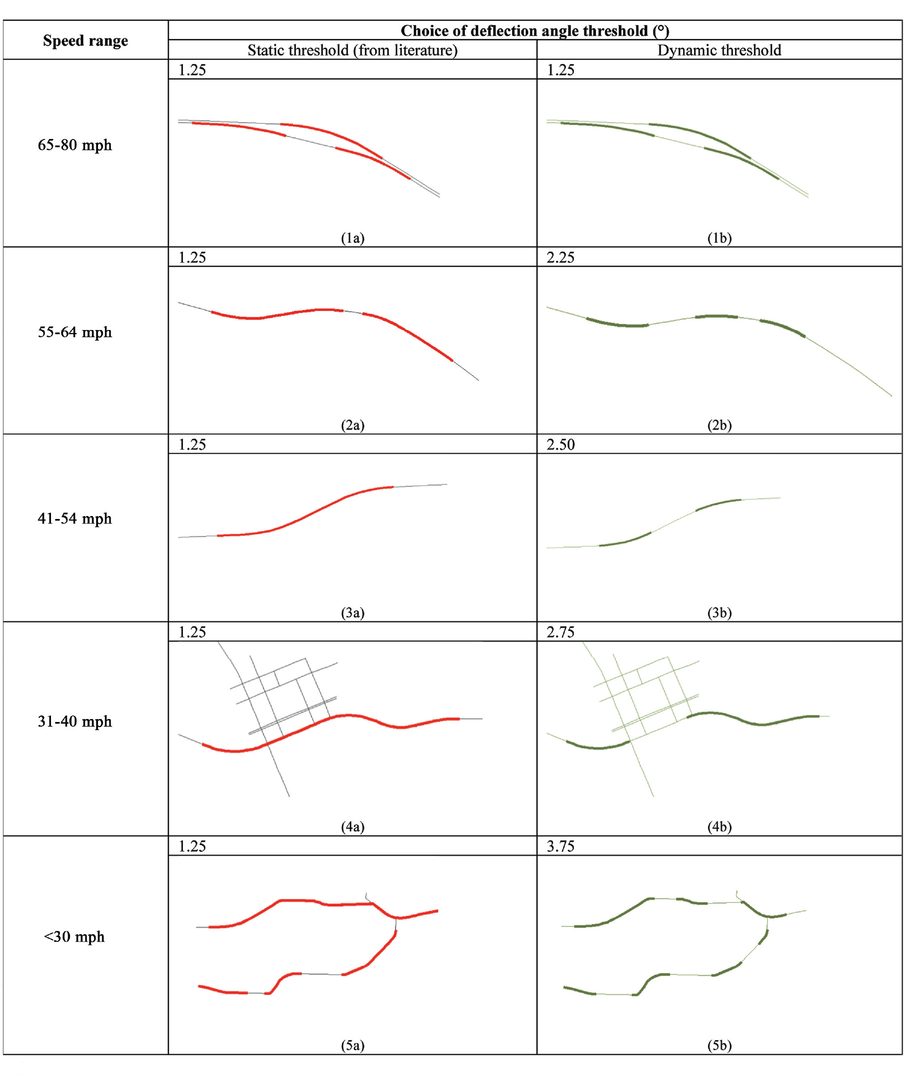
Dynamic deflection angle thresholds for curve identification.
To optimize the dynamic threshold based on roadway speed, it was observed that the deflection angles of the vertices of the roadways changed with different speed ranges. Figure 11 shows the proportions of the deflection angles of all vertices of roadways by various speed ranges. On high speed roads, more vertices tend to have a small deflection angle, while for lower speed roads more vertices tend to have a larger deflection angle. This is consistent with the guidelines in the roadway design manual ( 27 ). Therefore, it was concluded that the deflection angle threshold should be inversely proportional to roadway speed. Lower speed roads tend to have a higher threshold angle, and higher speed roads tend to have a lower threshold angle as it relates to curve determination.
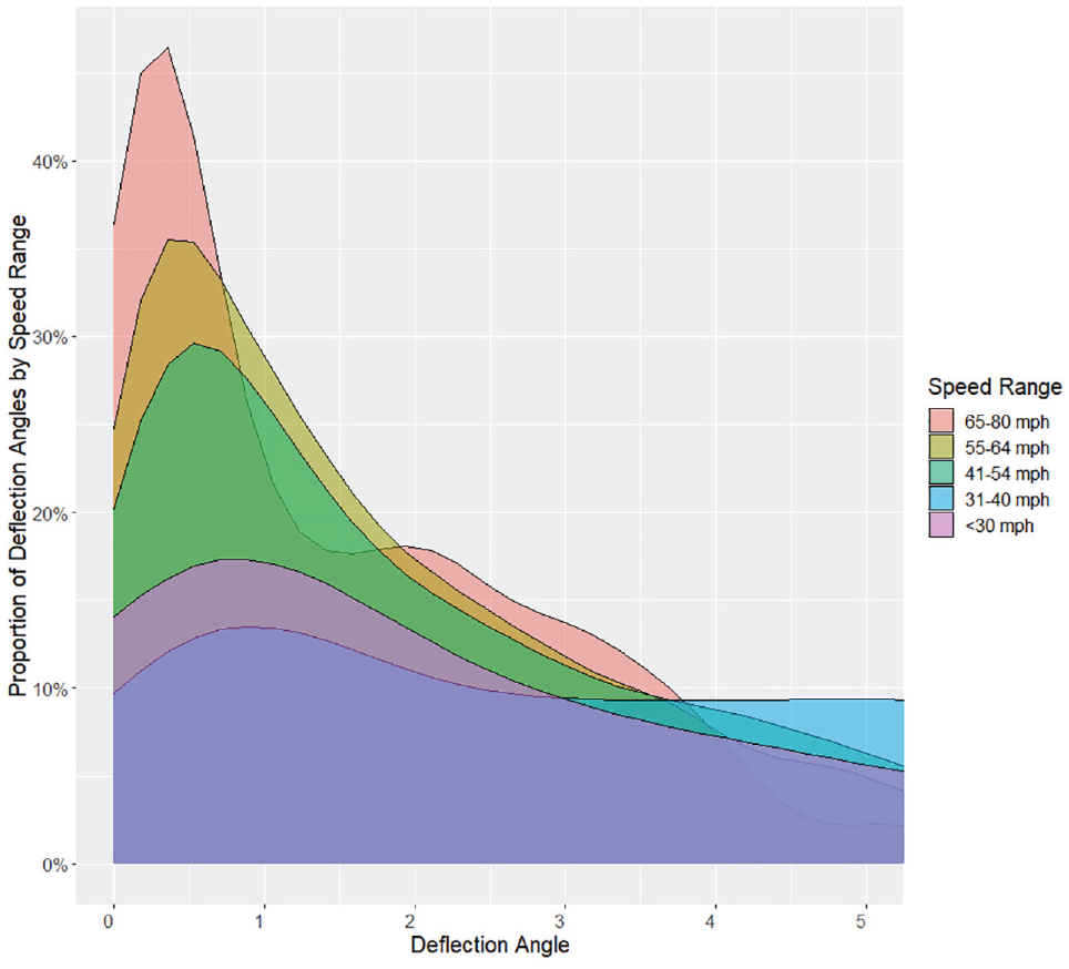
Proportion of deflection angles of vertices in roadways of various speed ranges.
Different thresholds were tried for different speed ranges and the optimal set was determined by observing the changes of resulting curves. For the high speed roads (above 55 mph), the aim was to create single continuous curves instead of multiple curves separated by small straight segments. For the low speed roads (below 30 mph), the aim was to create curves with shorter straight ends. The outcome is presented in Table 1, which shows the association between posted speed listed in the GIS street basemap and deflection angle threshold.
Dynamic Thresholds Related to Speed Ranges

Second, vertex density has an inverse relationship with the deflection angle threshold. Consider a circular arc of 1,000 ft in length that curves 60 degrees. If the arc is digitized with one vertex per 100 ft, there will be 10 vertices with an average deflection angle of 6 degrees. If that same arc is digitized with two vertices per 100 ft, there will be 20 vertices with an average deflection angle of 3 degrees. Roadways with higher vertex densities should have lower threshold angles and vice versa.
Further, an uneven distribution of vertices was observed along the centerline length, that is, vertices tended to cluster on curved roadways and disperse on straight roadways. To examine the vertex clustering, k-means clustering algorithm was utilized because it is a commonly used technique to determine the clustering of spatial points along linear networks ( 28 ) and therefore it is suitable in this case to incorporate in calculations of the deflection angle threshold in the proposed method.
The k-means algorithm partitions the objects into k clusters so that each object belongs to the cluster with the nearest centroid (
29
). By analogy, the curve’s vertices are considered as the objects and the curves are considered as the clusters. The k-means algorithm was implemented as follows. First, it selected the value of k using the rule of thumb: k =

where E is the sum of the squared error (distance from centroid) for all vertices in a polyline; p is the vertex; and ci is the centroid of a cluster.
For each cluster, the algorithm computed a new centroid using the vertices assigned to the cluster in the previous iteration. Vertices were then reassigned to clusters based on the distance to the new cluster centroids. The iterations continued until the vertex cluster assignments became stable, meaning that the clusters formed in the current iteration were the same as those formed in the previous iteration ( 29 ), that is, no vertex “moved” to a closer cluster centroid.
The deflection angle threshold was adjusted by comparing the vertex density for each cluster with the standard vertex density. The vertex density per 100 ft for each cluster is denoted as DC. The standard vertex density D0 is 1, meaning one vertex per 100 ft. Based on Table 1, the speed range of the roadway determines the threshold deflection angle of the vertex, denoted as the unadjusted threshold Tun-adj. Then, the adjusted threshold deflection angle would be

The effect is to adjust the threshold deflection angle inversely and proportionally to deviations in vertex density from the standard density, resulting in more accurate identification of curves and compensating for any inconsistencies in roadway centerline digitization.
Method to Determine a Dynamic Straight Segment Length Threshold for Compound and Reverse Curves
A compound curve is defined as a curve that consists of two circular arcs joined at a PT and that are on the same side of a common tangent ( 30 ), as shown in Figure 12a. Given that in GIS curves are in fact a series of consecutive straight lines joined at vertices, there is no ideal compound curve with two perfectly connected curved segments in a GIS street network. A compound curve in GIS needs to contain at least two curved segments connected with a straight segment (Figure 12b).
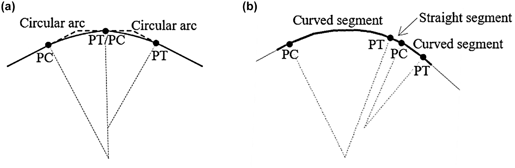
Ideal compound curve and GIS compound curve: (a) ideal compound curve with two arcs and (b) compound curve in GIS with two curved segments and a straight segment.
The length threshold of the straight segment is a critical factor that can determine if the consecutive curved segments should be considered as one compound curve or two independent curves instead. The literature providing guidance for the straight segment length threshold in regard to this issue is sparse. MIRE, AASHTO, and other U.S. national manuals provide little information on this threshold. Some DOTs ( 30 , 31 ) have more detailed straight segment length requirements but they are based on superelevation transitions information, which is not available in most GIS street basemaps. The only reference the authors could find is a constant of 600 ft threshold length—about 6 s drive for a vehicle traveling at 70 mph ( 22 ). However, this static threshold is not suitable for roads with different speeds. Lamm et al. ( 32 ) attempted to relate straight segment length to speed. However, the estimation was based on the 85th percentile speed, which is not available in GIS street basemaps, and the recommendations may not be reliable because they referred to older traffic conditions.
In the absence of specific guidelines, the authors turned to observations to develop a relationship between the maximum length of the straight segment and the roadway speed. When driving on a high speed road, it is obvious that the driver needs more distance to adjust from the straight roadway segment to the curved roadway segment. On the other hand, when driving on a low speed road, the driver needs less distance to adjust from the straight to the curved part. Therefore, a variable straight segment length was determined based on the roadway speed instead of using the constant length of 600 ft. Using a static straight segment length threshold resulted in incorrect determination of curves. They include the straight segments between two consecutive curves of high speed roads, such as state highways (Figure 13-2a), while covering almost the entire road on low speed roads (Figure 13-5a). These issues were corrected when using a dynamic threshold based on the speed of the roadway (Figure 13-2b–5b). Using observations on the GIS street basemap, a variable threshold length based on speed was developed, presented in Table 1 as the straight segment length threshold. From the literature ( 33 ), it can be inferred that 6 to 8 s is sufficient for the 85th percentile of drivers to react to unexpected complex information encountered during driving. Based on this information, the straight segment between curved segments should be long enough to allow most drivers 6 to 8 s to react by changing driving direction from a straight line to a curve.
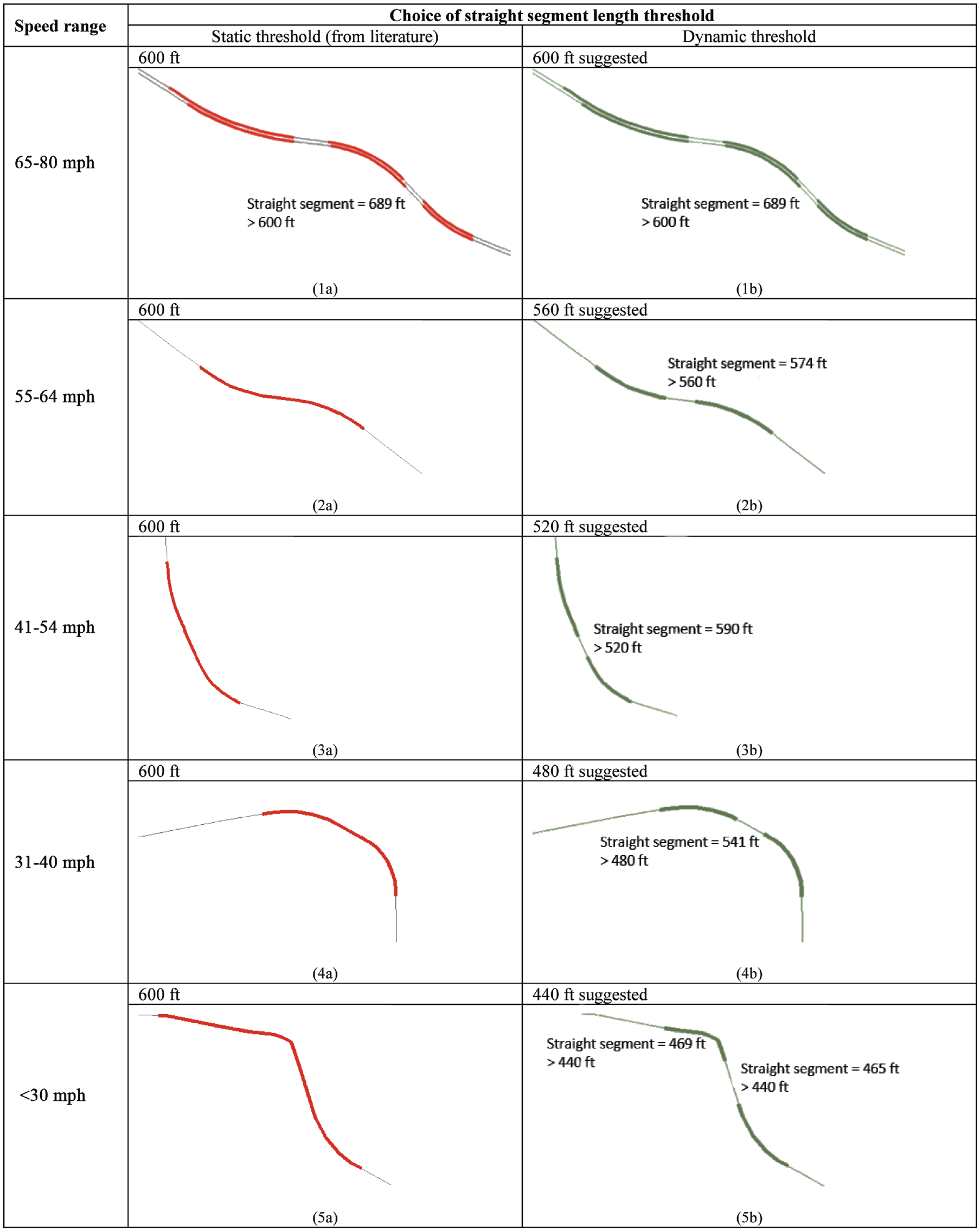
Dynamic straight segment length thresholds for curve identification.
Results and Validation
This method was applied to all the public roads in Florida, with a total GIS centerline (single and dual) length of over 200,000 miles. It identified more than 200,000 curves, 36,000 of which are located on state-maintained roads and 164,000 on local roads. Figure 14 shows an example of curves on state-maintained roads in one of the Florida’s 67 counties. The length of the majority of the curves ranges from 115 ft to 0.5 mile, and radius ranges from 50 ft to 0.4 mile.
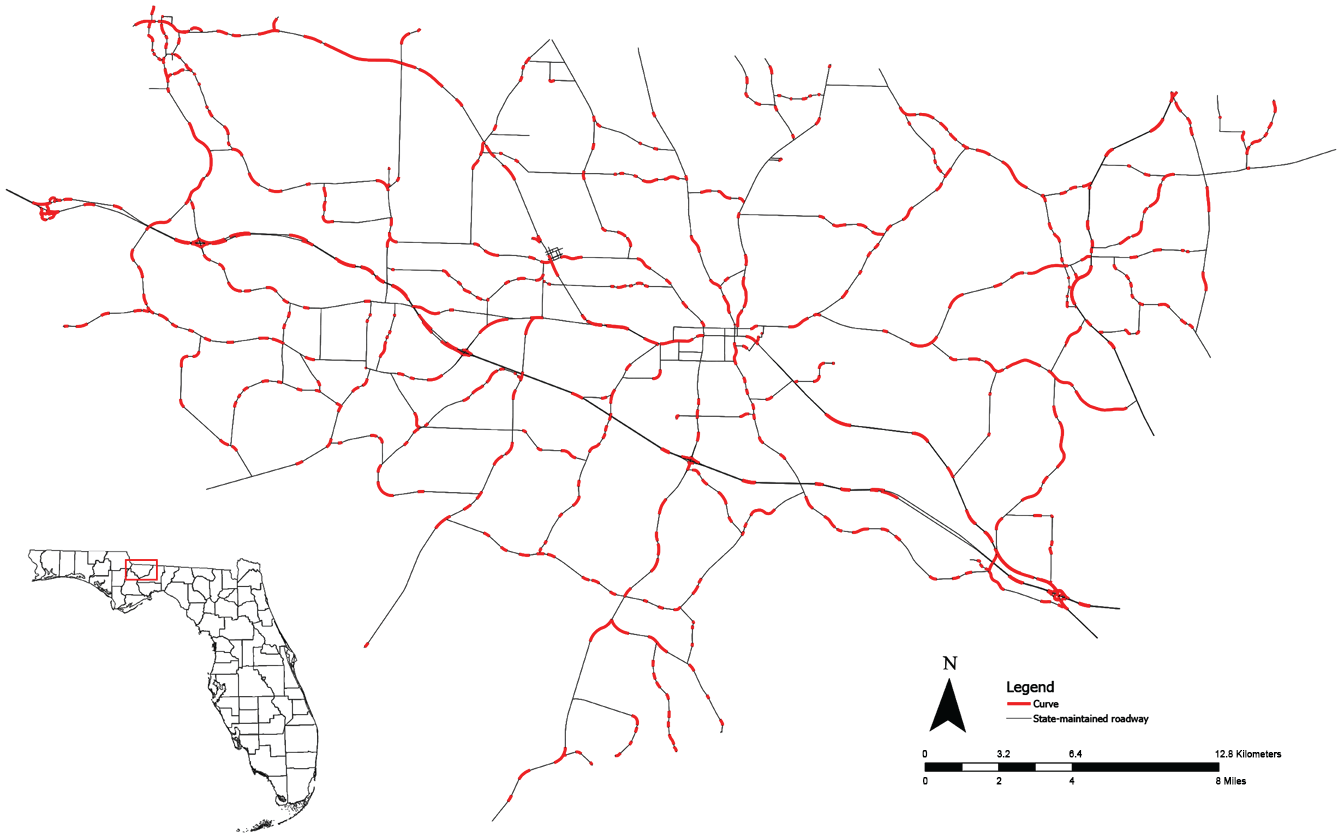
Curves on state-maintained roadways in Gadsden County, Florida.
The method has undergone extensive testing and was found to be operational. The method is computationally efficient. It can be executed at any time on demand. For an average county size with a GIS street basemap with around 500 miles of single and dual centerline of state-maintained roads, it takes only a few minutes to generate the curves on a computer with an Intel Xeon 2.6 GHz processor and 8 GB of RAM.
As mentioned earlier in this paper, there were no ground truth curves available for the validation of the results using a precise quantitative comparison. To overcome this limitation, two alternative methods were applied for the verification of the results: visual inspection using aerial photography and analytical comparison of curves with the theoretical circular arc.
Visual Inspection Using Aerial Photography
To perform a qualitative validation of the results by visually inspecting the curves using the aerial photography, a random spatially distributed set of curves was selected using the Geospatial Modelling Environment tool ( 34 ). The samples were randomly selected, including 75% (27,000) of curves on the state-maintained roads and 5% (8,200) of curves on local roads. The state-maintained curves were the primary focus. Therefore, a large sample of curves were inspected to detect the problematic ones and ensure the quality of the curve identification outcome. Additionally, the GIS roadway centerlines were inspected to confirm that the method did not miss any curves. The identified curves were visually compared with the curves on the roadways shown on the aerial photography. Findings revealed two types of issues: (a) correctable, which represented curves determined incorrectly by the proposed method. These were specific issues related to single/dual centerline split-merge points. The method was modified to correct the problem by skipping these points, as explained earlier in this paper; (b) uncorrectable, which were mainly poorly digitized centerlines or centerlines with very low vertex density. These indicate issues with the quality of GIS roadway centerlines, not with the method.
Results showed that 94.9% of state-maintained curves inspected were valid, and the remainding 5.1% were not curves. In local roads, 90.1% of curves inspected were valid, and the remainding 9.9% were not curves. The non-curve cases included turning lanes, the path to a cul-de-sac, curvy road segment inside a parking lot, or segments that wobble at intersections (Figure 15). These curves were also incorrectly identified because of the digitization quality of the GIS street basemap, not because of the method.
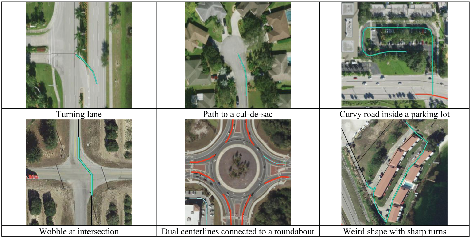
Examples of non-curve cases determined by visual inspection using aerial photography.
Comparison to Theoretical Circular Arc
To assess the quality of the identified curves and curve components, specifically the “curved segment” whose attributes such as PO, PI, PC, PT, central angle, and radius were largely derived from the geometry of a circle, a goodness of fit metric was developed to measure how well the curve polyline was fitted to a theoretical circular arc (Figure 16).
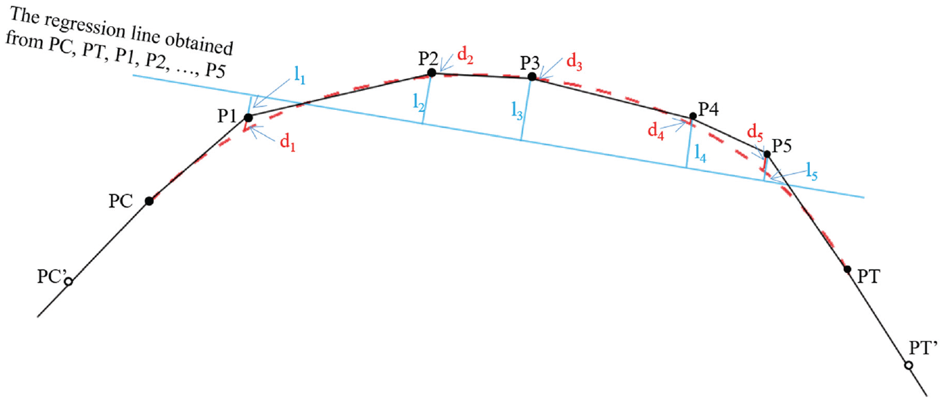
Diagram of goodness of fit indicating circle fitted with polyline.
The black polyline, representing the roadway segment, and the red line, representing the theoretical circular arc, are calculated from the coordinates of PC and PT. The other points P1, P2, …, P5 are the vertices of the polyline. The blue line represents the linear regression line fitted from PC, PT, P1, P2, …, P5. The goodness of fit is calculated as the ratio

where di is the distance from the vertices to the arc (d1, d2, …, d5) and li is the distance from the vertices to the regression line (l1, l2, …, l5)
Values closer to 1 represent a good fit, while values close to 0 or smaller represent a bad fit. The goodness of fit calculation was applied to each curved segment. Curves on state-maintained roads have an average of goodness of fit of 0.972, very close to a perfect 1, indicating a good fit of the roadway polylines to the theoretical circular arcs. Curves on non-DOT roads have an average of 0.874 goodness of fit. The bad fit curves are mostly the result of the poor digitization of the GIS basemap.
Discussion
From the methodological perspective, the final algorithm was a product of several iterative optimization and validation efforts, incrementally applied to larger geographic areas. The initial iteration was applied to one county, followed by more iterations applied to six pilot counties that represented a cross-section of rural and urban areas. The subsequent iterations improved the curve identification and optimized the parameters, such as the dynamic deflection angle threshold and straight segment length threshold. The finalized algorithm was applied to the entire state.
One thing to note is that this curve identification method is very low in cost. The only data requirement is a basemap of GIS roadway centerlines with a roadway identifier. These data nowadays are ubiquitous. The identifier, either a roadway ID of an LRS system, or a street name, is used for dissolving the original geometry segmentation of the basemap to create long continuous polylines (stored in the route layer), which allow the algorithm to trace the GIS centerlines from vertex to vertex. The use of the ID of the LRS, which created much longer route polylines than using the street name, has the advantage of producing a smaller number of polyline routes and more accurate continuous polyline delineation. This reduces the number of iterations, speeds up the process, and increases the accuracy of the results.
Another factor influencing the process of curve identification is the quality of the GIS roadway centerlines. While this method should work on any GIS street basemap with a roadway identifier, it creates more accurate curve outputs if the GIS street basemap is of a higher digitization quality, that is, more vertices are used to shape the roadway centerlines. Theoretically, it only takes at least three vertices to construct a curve. But the more vertices there are on a curve, the more accurate the curve is to the circular arc. In this study, it was noticed that the state-maintained road centerlines have a greater number of vertices than the local roads and the results reflect this difference. For example, it was observed that curves on freeways have an average of 8.75 vertices per curve, and the curves on local roads have an average of 5.87 vertices per curve. The method of applying dynamic thresholds helped to minimize the issues of data quality differences within the basemap.
While using reference curves determined on the ground by various technologies would be ideal as a reference for comparison with the curves determined from GIS centerlines through this automated method, it should be noted that for large geographic areas—such as the statewide extent in this study—the amount of ground data required for a meaningful validation may not be feasible because of the large effort and time required to collect them. Because of the great variation among roadways within the state, it would be very difficult and costly to select the roadway samples and collect the ground truth curves as representatives of the roadways statewide. Instead, the visual inspection of curves using aerial photography as a reference, coupled with the analytical validation method described above, confirmed that the improved method was able to identify curves using GIS roadway centerlines accurately.
Conclusion
The automated curve identification method presented here is accurate, low cost, uses widely available GIS data, requires minimal data processing, and executes rapidly. As such it is most useful for creating GIS curve inventories for large areas that can be used to support broad studies in traffic safety or to enhance basemaps for autonomous vehicle navigation. While this study draws from previous achievements, when comparing the approach presented here with previous methods, the following differences and improvements are observed:
The method presented here is better suited to identify curves on complex basemaps that use dual centerline for the representation of the GIS streets. The utilization of the LRS system associated with the GIS street basemap is an improvement in creating the continuous route polylines more accurately by dissolving on route identifiers. The method to exclude split-merge points is another improvement, specifically relevant to dual centerline basemaps.
A unique approach of this study is the structuring of the curve information in two layers: curve and curve component. By separating curve components from curves, it is possible to achieve a more precise radius calculation and more effective data management, and to provide the structure and information necessary to identify spiral transitions.
Spiral transition is difficult to detect because of its gradually changing radii and there are no documented efforts in the literature for automatic identification of spiral transition using GIS roadway centerlines. The spiral detection method developed in this study proved successful, although it is acknowledged that more in-depth study and improvements are needed in the future.
The method to determine the dynamic deflection angle threshold and straight segment length threshold makes this method adaptable to road networks of various classifications and speed ratings. Instead of a constant threshold, as indicated in previous studies, the method utilizes attributes from the GIS street basemap, such as roadway speed and vertex density, to improve the accuracy of curve identification. The method is also self-adjusting to compensate for uneven centerline digitization using the k-means clustering technique.
This study introduces an analytic validation method to evaluate the accuracy of the curve detection approach. A goodness of fit metric is applied to evaluate how well the curve (as-digitized representation) and the theoretical circular arc (as-designed representation) are fitted. The goodness of fit provides a standard metric to measure the quality of curve detection.
In conclusion, the methodology developed in this study shows a significant improvement compared with existing methods. It is able to identify the location of horizontal curves successfully for large geographic areas, is more accurate for calculation of curve attributes, and is more adaptable to handling various GIS roadway centerline representations and digitization of varying quality.
Footnotes
Author Contributions
The authors confirm contribution to the paper as follows: study conception and design: I. Bejleri; data collection: X. Xu, D. Brown; analysis and interpretation of results: I. Bejleri, X. Xu, N. Agarwal; draft manuscript preparation: I. Bejleri, X. Xu, S. Srinivasan. All authors reviewed the results and approved the final version of the manuscript.
Declaration of Conflicting Interests
The author(s) declared no potential conflicts of interest with respect to the research, authorship, and/or publication of this article.
Funding
The author(s) disclosed receipt of the following financial support for the research, authorship, and/or publication of this article: We would like to thank Florida Department of Transportation for funding this study.
