Departure Time Choice in Schedule-Based Transit Assignment

Abstract

This paper investigates existing departure time models for a schedule-based transit assignment and their parametrization. It analyzes the impact of the temporal resolution of travel demand and suggests functions for evaluating the adaptation time as part of the utility of a path. The adaptation time quantifies the time between the preferred and the scheduled departure times. The findings of the analysis suggested that travel demand should be discretized into intervals of 1 min, with interval borders right between the full minute, that is, ±0.5 min. It was shown that longer time intervals led to arbitrary run volumes, even for origin–destination pairs with just one transit line and a fixed headway. Although a linear relationship between adaptation time and adaptation disutility is a common assumption in several publications, it cannot represent certain types of passenger behavior. For some trip purposes, passengers may be insensitive to small adaptation times, but highly sensitive to large adaptations. This requires a nonlinear evaluation function.

Public transport assignment models are a fundamental tool in travel demand forecasting. They are used to determine passenger volumes in the transit network and to compute skim matrices describing the supply quality (e.g., travel time, number of transfers, cost) on the level of origin–destination (O-D) pairs. To achieve this, they must replicate the travel behavior and the resulting path choice of passengers as realistically as possible. Passengers collect information on the public transport supply provided by maps, timetables, and passenger information systems. Based on this information, they choose a suitable path through the network to reach their destination. As the availability and the quality of the transport supply are time-dependent, passengers must adapt their preferred departure time to the provided departure time.

Public transport assignment models can be divided into two main model classes ( 1 , 2 ):

Frequency-based assignment describes the supply of a transit line through the run time of the line route and the service frequency. The model is static as it assumes constant supply and demand during the assignment period. Passengers choose a path consisting of a sequence of lines based on their knowledge of line routes, travel times, and service frequencies. Each path provides exact in-vehicle times, but only expected waiting times and no discrete departure times. Model results provide volumes at the level of line routes.

Schedule-based assignment considers the timetable of each transit line with its exact departure and arrival times. The model is dynamic as it accounts for time-dependent supply and demand. Passengers choose a path consisting of a sequence of service runs based on their knowledge of the timetable. Each path has a discrete departure and arrival time, therefore providing exact information on in-vehicle time and transfer wait time. Model results provide volumes on the level of runs.

As frequency-based assignment is static, departure time choice is not an issue. This is different in schedule-based assignment: passengers can choose from a set of paths with exact departure and arrival times. Assuming that passengers have a preferred departure or arrival time, they need to select the path that best meets their temporal requirements. Such an approach is easy in cases in which all paths provide the same service quality (time, transfers, cost) and all paths are equally spaced in time. Then passengers either choose the path running before or after their preferred departure or arrival time. In cases with varying supply, for example, an occasional express service, the choice is more difficult. Passengers need to consider the service quality and the temporal suitability of a path. In both cases passengers choose a specific departure time. This leads to an adaptation time, which quantifies the time between the preferred and the scheduled time.

When implementing a schedule-based model, it is necessary to decide on the temporal resolution of the model. Service runs depart and arrive at discrete instants. It is common practice that timetables and timetable information systems indicate times in full minutes. Schedule-based models adopt this resolution for the supply model and the assignment graph. The definition of an appropriate temporal resolution for travel demand is less obvious. In trip diaries travelers often report their departure times rounded to 5, 10, or 15 min. For this reason, daily travel demand data are usually discretized into consecutive time intervals of a fixed duration, $τ$ . Within the time interval, demand is assumed to be equally distributed. When calculating time-dependent demand matrices with a travel demand model, typical interval durations are 60 min. For a dynamic highway assignment, shorter time intervals of 15, 10, or 5 min are common.

This paper investigates departure time models for a schedule-based transit assignment. It analyzes the impact of temporal resolution and suggests functions for evaluating the adaptation time as part of the utility of a path.

Related Work

Macroscopic travel demand models usually replicate the decisions of travelers with regard to their choices on traveling (trip generation), destinations, modes, and paths (assignment) within a typical day. Dynamic travel demand models and peak-hour models additionally disaggregate travel demand by time of day.

Cambridge Systematics ( 3 ) documents methods for including time of day issues in traditional four-stage modeling approaches. A common method derives the initial time interval for a person trip from the trip purpose. To establish time-dependent demand matrices for the assignment step, the demand matrix of a trip purpose (e.g., to work) is combined with an observed temporal distribution for this trip purpose. This demand representation determines the preferred time of a trip and can be used to estimate hourly demand, for example, for a peak-hour assignment.

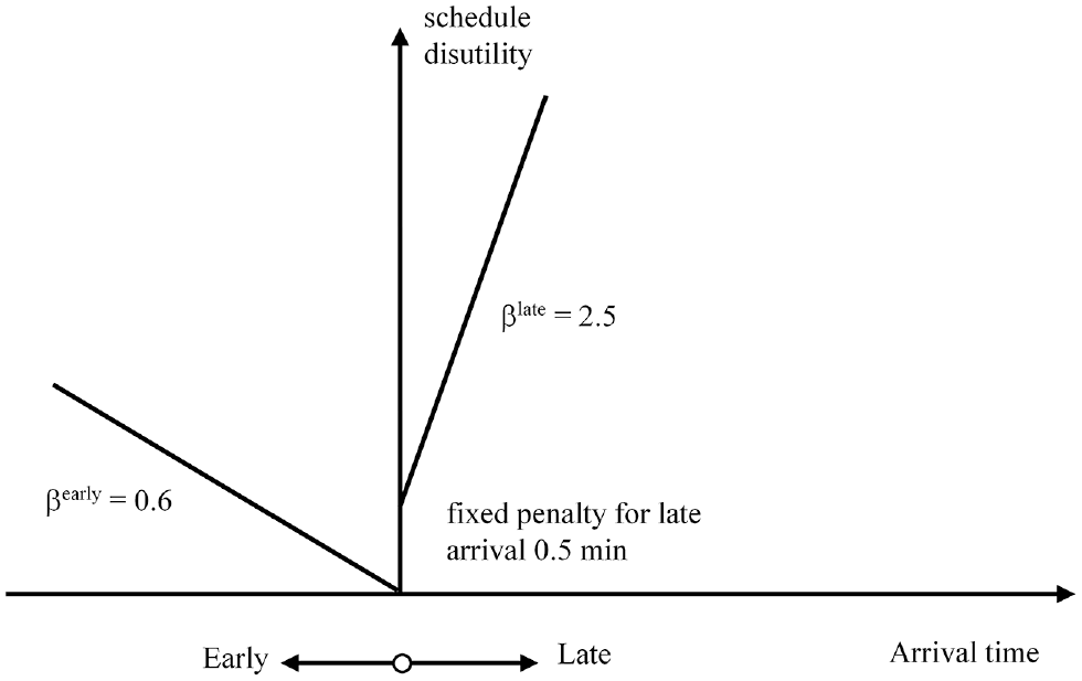
With the objective of incorporating time-dependent congestion levels in the network, the four-stage model can be amended by adding a time choice model. One way of doing this is to treat time choice as a discrete choice among time intervals. This requires a utility function for choices with variable departure time. For this purpose, Small introduces the terms early and late schedule delay, which quantifies the required adaptation time of travelers ( 4 ). Utility is maximized when travelers depart or arrive at their preferred time. Figure 1 shows an example for evaluating schedule delay with some parameter values from Ortúzar and Willumsen ( 5 ). Parameter values can be estimated using stated and revealed preference techniques. Fox et al. review studies of time period choice modeling, comparing the type of data (revealed, stated), the duration of time intervals, and the model structure ( 6 ).

Figure 1.

Schedule disutility (equivalent in minutes of travel time) for trips to work based on Small ( 4 ) and Ortúzar and Willumsen ( 5 ).

If time intervals are short, a model with departure time choice allows analysis of the peak spreading effects. For this, Arnott et al. integrate time choice into equilibrium models for highway assignment ( 7 ). Bellei et al. describe a demand model in which they integrate departure time choice into a nested logit model with five choice levels (travel, destination, mode, departure time, and path) ( 8 ). As they model public transport with frequencies, they avoid explicit path enumeration by adopting a continuous version of the logit model for the departure time choice. To determine the specific utility of departing at a given time, Bellei et al. assume that the utility is proportional to the difference between the preferred and given time.

In a schedule-based environment the supply is not continuous, but offers services at discrete points in time. In such cases it seems reasonable to assume that departure time and path choices are made jointly. This leads to a set of discrete choices for each O-D pair, which is equal to the number of time intervals multiplied by the number of paths ( 8 ). This approach is taken for example by Friedrich et al. ( 1 ). After a search step for identifying suitable paths in a schedule-based graph, the choice step is performed for every time interval. Using a multinomial logit model, the utility of a path includes the service quality (time, transfers), the fare, and a temporal utility. Similar to Small ( 4 ), the temporal utility function evaluates the difference between the preferred and the provided departure time of the path. The utility is 0 for paths departing within the time interval and decreases monotonically for paths departing outside the time interval, that is, these paths are penalized. The paper does not suggest values for the duration of a time interval and the form of the temporal utility function. A similar model formulation can be found in Chapter 6.3.7 of Gentile at al. ( 2 ). Here again a linear expression with different coefficients for early and late departure is suggested for determining temporal disutility, similar to Figure 1.

Since paths in a public transport network may overlap in space and time, the IIA (independence of irrelevant alternatives) condition required by the logit model is usually not fulfilled. As a method of capturing similarities of alternatives in schedule-based assignment, Friedrich et al. propose the concept of independence ( 1 ). Similar to the C-logit model, this concept adapts the utility of a path depending on its departure and arrival time.

The problem of overlapping alternatives does not apply to the rooftop model described by Douglas et al. ( 9 ). The model’s name comes from the graph of the time-dependent impedance function, which is shaped like rooftops. The rooftop model builds on a time-dependent shortest path search. For each preferred departure time instant, the demand is assigned to the path that minimizes the impedance, which is a linear combination of service quality (journey time) and adaptation time.

Contribution

This paper investigates departure time models for a schedule-based transit assignment. Building on Friedrich et al. ( 1 ), a model formulation that integrated departure time and path choice was considered. The impact of the temporal resolution on the model was analyzed. This revealed that discretizing the travel demand into long intervals led to arbitrary run volumes, even for O-D pairs with just one transit line and a fixed headway. To prevent this, the temporal resolution of the travel demand should match that of the timetable (e.g., 1 min). Whereas previous publications assumed a linear relationship between adaptation time and adaptation utility, this paper demonstrates that this cannot represent certain types of passenger behavior. For some trip purposes, passengers may be insensitive to small adaptation times, but highly sensitive to large adaptations. This requires a nonlinear evaluation function.

To focus on these topics in the analysis, the paper assumes two simplifications:

The presented model formulation considers only the distribution of the preferred departure times and the actual departure times provided at the origin. If demand is specified for a preferred arrival time at the destination (e.g., trip purpose work or education), the same model formulation can be applied in relation to arrivals.

The impacts of congestion are not considered in the model formulation. Overcrowding on specific sections of a run may influence path choice and thus departure time choice. For this to be achieved, the model formulation would have to be extended to include a discomfort term.

Departure Time Model Formulation

The considered departure time model builds on the framework described in Friedrich et al., which integrates departure time choice and path choice at the level of an O-D pair ( 1 ). It requires the following input:

A set of runs $r \in R$ , where each run describes the time–space trajectory of a vehicle from the origin terminal to the destination terminal.

A set of paths $k \in K$ , where each path describes the time–space trajectory of a journey from an origin zone to a destination zone. The journey has a specific departure time, $d_{k}$ , at the origin and a specific arrival time at the destination. Each path concatenates one or more run sections. The set of paths can either be computed explicitly using a schedule-based path generator (e.g., the branch-and-bound algorithm for choice-set generation described in Friedrich et al. [1]) or it can be represented by arc conditional probabilities resulting from a sequential model with an implicit enumeration of paths ( 2 ). One example of an arc-based model with implicit enumeration is described in Briem et al. ( 10 ).

Travel demand for each O-D pair. This demand is divided further by demand group and departure time interval. All passengers within a demand group, $g$ , share the same trip purpose (work, shopping, etc.) and the same preferences when evaluating the utility of a path.

Departure Time Interval Refinement

Travel demand data are discretized into consecutive time intervals of a fixed duration τ (e.g., 1 h). Formally, a departure time, d, specified in the demand corresponds to a departure time interval $[d, d + τ]$ . In Friedrich et al., this interval is interpreted as the range of departure times preferred by the passengers with departure time d ( 1 ). For paths whose actual departure time falls outside this range, an adaptation time is calculated as the difference between the actual departure time and the closest boundary of the interval. The temporal utility of the path is penalized according to the adaptation time. Departures within the interval are not penalized.

The shortcoming of this approach is to assume that the temporal resolution of the demand data corresponds to the range of departure times preferred by the passengers. To eliminate this shortcoming, the input intervals are refined into smaller intervals of a fixed duration, δτ, such that τ is a multiple of δτ. Given an input interval $[d, d + τ]$ with m passengers, the interval is divided into $n = τ / δ τ$ slices with $m / n$ passengers each, where slice i corresponds to the interval $[d + i \cdot δ τ, d + (i + 1) \cdot δ τ]$ of preferred departure times. For $δ τ \to 0$ , this leads to a continuous temporal distribution of the demand, such that each passenger has a singular preferred departure time.

Adaptation Time

Given a path, k, and an interval $[d, d + δ τ]$ of preferred departure times, the early adaptation time, $Δ t_{k, d}^{early}$ , and late adaptation time, $Δ t_{k, d}^{late}$ , represent the difference between the provided departure time, $d_{k}$ , and the preferred departure time. The early adaptation time, $Δ t_{k, d}^{early}$ , is non-zero if $d_{k}$ lies before the earliest preferred departure time, d, whereas the late adaptation time, $Δ t_{k, d}^{late}$ , is non-zero if $d_{k}$ lies after the latest preferred departure time, d+δτ. Formally, they are defined as follows:

\begin{matrix} Δ t_{k, d}^{early} = max (0, d - d_{k}) \\ Δ t_{k, d}^{late} = max (0, d_{k} - (d + δ τ)) \end{matrix}

(1)

Utility Model

The utility model follows a standard formulation for evaluating public transport service quality based on perceived journey time. It is supplemented by penalties for early and late departure. The perceived journey time, $t_{k, g}^{PJT}$ , of a path, k, for a demand group, g, is calculated as follows:

t_{k, g}^{PJT} = β_{g}^{IVT} \cdot t_{k}^{IVT} + β_{g}^{AET} \cdot t_{k}^{AET} + β_{g}^{TWT} \cdot t_{k}^{TWT} + β_{g}^{NoT} \cdot n_{k}^{NoT}

(2)

$β_{g}^{IVT}$ = parameter for in-vehicle time,

$t_{k}^{IVT}$ = in-vehicle time of path k,

$β_{g}^{AET}$ = parameter for evaluating access, egress, and transfer walk time,

$t_{k}^{AET}$ = access, egress, and transfer walk time of path k,

$β_{g}^{TWT}$ = parameter for evaluating transfer wait time,

$t_{k}^{TWT}$ = transfer wait time of path k,

$β_{g}^{NoT}$ = parameter for evaluating number of transfers, and

$n_{k}^{NoT}$ = number of transfers in path k.

Together with penalty terms for travel fare and adaptation time, the perceived journey time is a component in the impedance of a path. Given a path, k, a demand group, g, and a departure time interval, $[d, d + δ τ]$ , the impedance, $w_{k, g, d}$ , is defined as follows:

\begin{matrix} w_{k, g, d} = β_{g}^{PJT} \cdot t_{k, g}^{PJT} + β_{g}^{c} \cdot c_{k, g} + β_{g}^{early} \cdot f_{g}^{early} (Δ t_{k, d}^{early}) \\ + β_{g}^{late} \cdot f_{g}^{late} (Δ t_{k, d}^{late}) \end{matrix}

(3)

where

$β_{g}^{PJT}$ = parameter for evaluating perceived journey time,

$t_{k, g}^{PJT}$ = perceived journey time of path k for demand group g,

$β_{g}^{c}$ = parameter for evaluating cost (travel fare),

$c_{k, g}$ = cost (travel fare) of path k for demand group g,

$β_{g}^{early}$ = parameter for evaluating early departure,

$f_{g}^{early}$ = early adaptation time evaluation function: maps early departure adaptation time to adaptation penalty,

$Δ t_{k, d}^{early}$ = early departure adaptation time,

$β_{g}^{late}$ = parameter evaluating for late departure,

$f_{g}^{late}$ = late adaptation time evaluation function: maps late departure adaptation time to adaptation penalty, and

$Δ t_{k, d}^{late}$ = late departure adaptation time.

Since the impedance is inversely correlated with the usefulness of a path, the utility, $v_{k, g, d}$ , is defined as the negative impedance,

v_{k, g, d} = - β \cdot w_{k, g, d}

(4)

Here, β is a general scaling factor, which controls the impact of the randomly distributed component of the utility in a discrete choice model, for example, a logit model.

Adaptation Time Evaluation Functions

The adaptation time evaluation functions $f_{g}^{early}$ and $f_{g}^{late}$ transform the early and late adaptation times $Δ t_{k, d}^{early}$ and $Δ t_{k, d}^{late}$ into penalties that are added to the impedance of a path. If the provided departure time lies within the interval of preferred departure times, it ensures that the adaptation penalty is 0 because $Δ t_{k, d}^{early}$ and $Δ t_{k, d}^{late}$ will be 0. In line with Friedrich et al. ( 1 ), $f_{g}^{early / late}$ must be a monotonically increasing function (i.e., a higher adaptation time leads to an equal or higher adaptation penalty). However, instead of $f_{g}^{early / late} (Δ t) > 0$ for $Δ t > 0$ , it is sufficient to only require $f_{g}^{early / late} (Δ t) \geq 0$ . This makes it possible to extend the interval in which departures are not penalized beyond $[d, d + δ τ]$ , if desired.

The simplest modeling assumption is that the adaptation penalty is proportional to the adaptation time. This results in a linear evaluation function,

f_{g}^{early / late} (Δ t) = Δ t

(5)

It is not necessary to include a scale parameter that controls the slope of the function, since this is already accomplished by the scaling parameters $β_{g}^{early}$ and $β_{g}^{late}$ .

Although a linear relationship between adaptation time and adaptation penalty is a natural assumption, it cannot represent certain types of passenger behavior. For some trip purposes, passengers may be insensitive to small adaptation times, but highly sensitive to large adaptations. This can be modeled with a higher degree polynomial. The simplest example for a polynomial with degree λ > 1 is the following:

f_{g}^{early / late} (Δ t) = Δ t^{λ}

(6)

It may also be desirable to increase the duration of the interval in which an early or late departure is not penalized. This can be achieved by shifting Δt downward by some offset x in the evaluation function,

f_{g}^{early / late} (Δ t) = (max (0, Δ t - x))^{λ}

(7)

Since the evaluation functions are dependent on the demand group, g, it is possible to tailor the functions to the particular trip purpose of each group. Furthermore, whereas choosing the same function for both $f_{g}^{early}$ and $f_{g}^{late}$ is sufficient in many cases, there are some trip purposes for which it is more realistic to choose different functions. For example, when traveling to work, late departures beyond a certain point are heavily penalized as the passenger will be late for work, whereas early departures should be penalized more lightly.

Decision Model Types

Given a choice set $K = {k_{1}, \dots, k_{n}}$ of paths with observed utilities $v_{1}, \dots, v_{n}$ , the decision model determines the probabilities $P_{1}, \dots, P_{n}$ that each option is chosen by a passenger. In the following, two types of decision models are considered: the multinomial logit model and the rooftop model.

The multinomial logit model is a widely used random utility model that assumes that the overall utility, $u_{i}$ , of each option, $i$ , consists of the observed component, $v_{i}$ , and an unobserved component, $ε_{i}$ , yielding $u_{i} = v_{i} + ε_{i}$ . The unobserved components are random variables that are independently and identically distributed according to a Gumbel distribution. The resulting probabilities can then be calculated as follows:

P_{i} = \frac{e^{v_{i}}}{\sum_{j = 1}^{n} e^{v_{j}}}

(8)

By contrast, the rooftop model assumes that passengers always choose the option that maximizes their observed utility. In cases where the maximum observed utility is shared by multiple options, they are chosen with equal probability,

\begin{matrix} P_{i} = \\ {\begin{matrix} 1 / | {i | v_{i} = max (v_{1}, \dots, v_{n})} | & if v_{i} = max (v_{1}, \dots, v_{n}) \\ 0 & otherwise \end{matrix} \end{matrix}

(9)

The rooftop model is used in conjunction with linear evaluation functions for the adaptation penalties, that is, $f^{early / late} (Δ t) = Δ t$ .

Comparison of Departure Time Model Variants

Example Network and Demand Structure

To illustrate and to analyze the different possible choices for the evaluation function for Δt and the decision model in the model formulation, a simple network with two lines and a demand structure for one O-D pair is sufficient (Figure 2). The demand is given for the time period between 7:00 and 8:00 a.m. and is assumed to be equally distributed within this hour. Two public transport lines connect origin and destination. The regular line (R) has a perceived journey time (PJT) of 20 min and runs every 15 min (first run at 6:40 a.m., last run at 8:25 a.m.). The express line (E) is faster (PJT = 15 min) but offers only one run at 7:34 a.m. There are two supply scenarios: The base scenario (B) only contains Line R whereas the express scenario (E) additionally includes Line E. Since the network does not include any transfer stops, each run, r, corresponds to one path, k.

Figure 2.

Example network and timetable.

Considered Cases and Parameter Settings

The examined cases vary the model settings in four ways:

Supply scenario: base scenario (B) and express scenario (E)

Temporal resolution of the demand period: one interval of 60 min, six intervals of 10 min and 60 intervals of 1 min.

Decision model: multinomial logit model (L) or rooftop model (R). In the presented cases, the logit model is applied straightforwardly without any corrections addressing the temporal similarity within the choice set, K.

Evaluation function for Δt: linear term according to Equation 5 with β^dep = β^early = β^late = 1 (L) or a polynomial of higher order according to Equation 6 with β^dep = β^early = β^late = 0.0002 and λ = 4 (P).

The combination of the two supply scenarios and the different model settings leads to 24 possible cases. A case is identified by the combination of the four variables. As an example, E_1′_L_P stands for the express scenario with 60 demand intervals of 1 min using the logit model with a higher order polynomial for the evaluation of the adaptation time, Δt.

In the following, the results of six selected cases are compared to illustrate the shortcomings of some common modeling approaches and to suggest suitable parameter settings. Figure 3 shows the aggregated result of the path choice for the six cases. It is apparent that the shares of each path differ considerably between some of the cases involving the express scenario. Figures 4 and 5 show the results of the six cases in detail in the order of the explanations in the following sections.

Figure 3.

Comparison of path choice results for the six selected cases.

Figure 4.

Impedance and path choice results of cases: (a) E_60′_L_L, (b) B_10′_L_L, and (c) B_1′_L_L.

Figure 5.

Impedance and path choice results of cases: (a) E_1′_L_L, (b) E_1′_L_P, and (c) E_1′_R_L.

Duration of Interval δτ

In travel demand modeling, observed and modeled demand data are often provided in time intervals of 1 h. This may lead to the assumption that the demand of a certain hour can freely choose its departure time within this time span. Such an assumption is made in all cases with only one interval of 60 min.

Figure 4ashows the impedance and the results for case E_60′_L_L. The left-hand diagram shows the impedance for each run as it is perceived by a person with a certain preferred departure time. For example, a person with the preferred departure time 7:10 a.m. perceives the service run E7:34 with an impedance of 15 min. The runs R7:10, R7:25, R7:40, and R7:55 are perceived with an impedance of 20 min. Owing to the interval duration of 60 min, all passengers with a preferred departure time between 7:00 and 8:00 a.m. evaluate the transport supply equally. As all these runs depart within the demand interval, the adaptation time, Δt, is 0 and the impedance is equal to the PJT. Run R6:55 is evaluated with an impedance of 25 min (20 min PJT, adaptation time Δt = 5 min, β^dep = 1). Run R8:10 with an adaptation time Δt = 10 min obtains an impedance of 30 min. The right-hand diagram in Figure 4a shows the share of the demand of each demand interval choosing a specific path. As this case covers only one interval, the path choice is identical for all trips departing between 7:00 and 8:00 a.m. The results reveal the problem of this model assumption, as the runs R7:10, R7:25, R7:40, and R7:55 receive equal shares of demand. Such a distribution is unlikely in reality. One would expect R7:25 to suffer more from the attractiveness of E7:34 than, for example, R7:10; R7:25 should therefore receive a smaller share of the demand compared with R7:10.

A temporal resolution with shorter time intervals, represented here by all cases with 10 min intervals, also leads to unsatisfactory model results. Figure 4b shows the results for one case of this group (B_10′_L_L). Considering the share of each path shown in Figure 3, it is noticeable that R7:25 attracts less demand than R7:10 and R7:40. The demand structure with an equally distributed preferred departure between 7:00 and 8:00 a.m. does not suggest such behavior. The reason for this can be found in the arbitrary determination of the interval boundaries and is visible in Figure 4b. R7:10 and R7:40 depart exactly at the border between two demand intervals. For both intervals, no additional impedance is added for the adaptation time, Δt, so that both receive a high share of demand from the adjacent intervals. Such variations in demand share are not appropriate in the case of a supply with fixed headways and a constant demand. Although the interval boundaries of the demand in this example network could be aligned with the supply, this is not possible when modeling a real public transport network. For this reason, this problem can only be avoided by choosing a temporal resolution for the demand intervals that is at least equal to the resolution of the timetable. If departure times of runs are given to the full minute, an interval duration of 1 min (with interval borders right between the full minute, i.e., ±0.5 min) has to be chosen.

An example with sufficiently small demand intervals is given in Figure 4c (B_1′_L_L). The demand distribution (Figure 3) shows a lower demand for paths that are close to the boundary of the demand period. The closer the paths are to the middle of the demand period, the more evenly the demand is distributed among them.

Evaluation Function for Δt

To justify the choice of a nonlinear function for evaluating the adaptation time, case E_1′_L_L with a linear evaluation function is considered first (Figure 5a). This case differs from the case shown in Figure 4c only in the supply with the express run added. Compared with the runs of the regular line, it has a 5-min lower PJT. Considering the path choice in the individual time intervals, it is noticeable that the demand for run E7:34 decreases sharply for small deviations from its departure time. At the same time, it can be seen that demand from more distant time intervals (e.g., between 7:00 and 7:10 a.m.) still uses run E7:34 with a nonnegligible probability. Such assignment results are not fundamentally wrong and can perhaps be observed in reality under certain circumstances. Nevertheless, it is plausible that the two runs R7:25 and R7:40 are influenced more strongly by the attractiveness of the faster E7:34. This assumes that there is some flexibility toward small deviations from the preferred departure times. At the same time, it can be assumed for many trip purposes that the adaptation time becomes more important, the bigger the difference between the preferred departure time and the realized departure time gets. In the example network, the time savings of 5 min provided by run E7:34 become less important with an increasing adaptation time.

To replicate such behavior, a modified evaluation function for the adaptation time, Δt, is applied. Figure 5b shows the impedance and the results for case E_1′_L_P. Considering the left-hand diagram, the impedance shows only a small increase for adaptation times close to the preferred departure time. In the presented case this applies to an adaptation time of approximately ±10 min. Beyond this, the reaction to increasing adaptation times is stronger. This short-term flexibility can be explained by the fact that short interim periods are usually easy to bridge. Large deviations from planned behavior, in contrast, may require an adjustment of the activity schedules and are less tolerable. The results in the right-hand diagram of Figure 5b show that run E7:34 attracts an almost constant share from demand intervals with a preferred departure between the two runs R7:25 and R7:40. In time intervals further from the departure time of E7:34, the demand share drops more steeply than in Figure 5a. For demand intervals at the edges of the demand period, E7:34 is no longer of importance.

It is obvious that departure time choice depends highly on the trip purpose. The suggested use of evaluation functions of higher order is supposed to allow better adaptation to real behavior. Figure 6 suggests possible parameter sets for two trip purposes. Ideally the parameters are estimated using observations from stated preference surveys.

Figure 6.

Possible parameter sets by trip purpose for a regional demand model.

Rooftop Model

The focus of the previous considerations has been on models that use a logit decision model. In the following, results for the rooftop model are presented. The results of a rooftop model with a linear evaluation function for Δt (E_1′_R_L) are shown in Figure 5c.

The progression of the impedance of each path over the preferred departure time is identical to that shown in Figure 5a. The illustration provides a good explanation of the decision-making process replicated by a rooftop model. The demand of one interval only sees the best option for exactly this time interval. Consequently, the entire demand is assigned to this option. This can be observed in the right-hand diagram in Figure 5c, in which the entire demand of a particular time interval uses the same path. The only exception is the interval 07:26:30 to 07:27:30, where the two paths R7:25 and E7:34 have equal impedance.

The impedance diagram in Figure 5c also shows the weakness of a rooftop model. For preferred departure times between 07:39:30 and 07:47:30, path R7:40 has a minimal advantage over the express path E7:34. Therefore, path E7:34 is not assigned any demand during this period, which is not likely to correspond to observed behavior. As a result, path E7:34 receives a remarkably lower share of the total demand compared with the logit approach (Figure 3).

In the rooftop model, the demand share of the express run strongly depends on its departure time (Figure 7, left-hand diagram). This is not the case in the logit model with a low departure time sensitivity. As the sensitivity increases (right-hand diagram), the dependence on the departure time becomes more pronounced for the logit model.

Figure 7.

Shares of total demand of express run for different departure times and two sets of model parameters with low and high departure time sensitivity.

Conclusions and Recommendations

The presented analysis shows the impact of the temporal resolution of demand and the choice of parameters for evaluating adaptation time on the assignment results. Most schedule-based model implementations in practice are likely to use time intervals >> 1 min and a linear evaluation of adaptation time. Such implementations will lead to arbitrary run volumes, even in cases with one line and a fixed headway. In cases in which passengers can choose between alternatives with different PJTs and headways, such an implementation will additionally influence aggregated volumes on the link level.

The findings of the analysis can be applied to most existing schedule-based transit assignment approaches to improve the level of realism in departure time choice modeling. These are summarized in the following recommendations:

If departure times of runs are given to the full minute, an interval duration of 1 min (with interval borders right between the full minute, i.e., ±0.5 min) has to be chosen;

Adaptation time should be evaluated using a nonlinear evaluation function, $f^{dep} (Δ t) = Δ t^{λ}$ ; and

If the model is applied to determine run volumes, parameters for evaluating adaptation time should depend on the trip purpose.

Improvements in departure time modeling are a prerequisite for determining saturation on the level of service runs. An assignment model formulation that considers capacity constraints should only be used if the model is able to produce valid saturation levels on a low level of aggregation.

To implement the recommendations derived from this paper in travel demand modeling (especially the use of nonlinear evaluation functions that are dependent on trip purpose), it will be necessary to find appropriate parameters for the model calibration. As the desired departure time is not captured in regular trip diaries or passenger surveys, this is work for future research to find applicable methods of data collection for parameter estimation. Nevertheless, the temporal disaggregation of demand can be applied without further data being required.

Footnotes

Author Contributions

The authors confirm contribution to the paper as follows: study conception and design: M. Friedrich, M. Schmaus, J. Sauer; data collection: M. Schmaus, J. Sauer; analysis and interpretation of results: M. Friedrich, M. Schmaus, J. Sauer; draft manuscript preparation: M. Schmaus, J. Sauer. All authors reviewed the results and approved the final version of the manuscript.

Declaration of Conflicting Interests

The authors declared no potential conflicts of interest with respect to the research, authorship, and/or publication of this article.

Funding

The authors disclosed receipt of the following financial support for the research, authorship, and/or publication of this article: This research was funded by Deutsche Forschungsgemeinschaft (DFG, German Research Foundation) as part of the research group for integrated planning in public transport FOR2083.

ORCID iDs

Markus Friedrich

Matthias Schmaus

References

Friedrich

Hofsäß

Wekeck

Timetable-Based Transit Assignment using Branch and Bound Techniques. Transportation Research Records: Journal of the Transportation Research Board, 2001. 1752: 100–107.

Gentile

Florian

Hamdouch

Cats

Nuzzolo

The Theory of Transit Assignment: Basic Modelling Frameworks. In Modelling Public Transport Passenger Flows in the Era of Intelligent Transport Systems ( Gentile

Noekel

, eds.), Springer Tracts on Transportation and Traffic, Springer International Publishing, 2016.

Cambridge Systematics, Inc. Time-of-Day Modeling Procedures Report. Travel Model Improvement Program, FHWA, 1997. https://www.fhwa.dot.gov/planning/tmip/publications/other_reports/tod_modeling_procedures/time-day.pdf. Accessed July 20, 2020.

Small

K. A.

The Scheduling of Consumer Activities: Work Trips. The American Economic Review, Vol. 72, No. 3, 1982, pp. 467–479.

Ortúzar

J. D.

Willumsen

L. G.

Modelling Transport. John Wiley & Sons, 2011.

Fox

Dunkerley

Patruni

Daly

Time Period Choice Modelling – Review of Practice. RAND Corporation. 2014. http://www.rand.org/pubs/research_reports/RR1127.html. Accessed July 20, 2020.

Arnott

De Palma

Lindsey

Departure Time and Route Choice for the Morning Commute. Transportation Research B: Methodological, Vol. 24, 1990, pp. 209–228.

Bellei

Gentile

Meschini

Papola

A Demand Model with Departure Time Choice for Within-Day Dynamic Traffic Assignment. European Journal of Operational Research, Vol. 175, 2006, pp. 1557–1576. https://doi.org/10.1016/j.ejor.2005.02.028.

Douglas

N. J.

Henn

Sloan

Modelling the Ability of Fare to Spread AM Peak Passenger Loads Using Rooftops. Proc., Conference Paper Delivered at the 34th Australasian Transport Research Forum (ATRF), Adelaide, Australia, 2011.

10.

Briem

Buck

Ebhart

Mallig

Strasser

Vortisch

Wagner

Zündorf

Efficient Traffic Assignment for Public Transit Networks. Proc., 16th International Symposium on Experimental Algorithms (SEA 2017). Schloss Dagstuhl-Leibniz-Zentrum fuer Informatik, 2017.

11.

PTV

AG.

PTV Visum 20 User Manual. 2019. https://www.ptvgroup.com/en/solutions/products/ptv-visum/. Accessed July 20, 2020.