



Abstract
This paper describes how human factors (HF) and user workload (WL) can be used by highway designers and traffic engineers to quantify the potential safety of sections of highway. Users’ WL is a quantitative measure of HF. Both HF and WL are used successfully in other fields, such as aviation when pilots have difficulty in using instruments and in touch-down before the start or end of the runway. The traditional highway approach of gauging success is by counting crashes. But with fatalities exceeding 30,000 a year for more than 20 years, the time is right for a new method of analysis. The author has integrated specific WL metrics into a simplified example to aid designers, traffic engineers, and safety analysts in assessing user problems before building new projects or road upgrades. The example uses static and dynamic WL and alternating renewal (AR) metrics (not used by others) to quantify user WL in highway segments for the purpose of illustrating the variation of design and operational safety conditions. The example can be easily modified when new metrics are created, and it illustrates the use of WL and its associated highway safety implications. In short, the approach is based on common sense with trained engineering experience and logic integrated into data-driven safety analyses. The example is a continuation of an earlier FHWA research study illustrating the application of road safety audits and the Interactive Highway Safety Design Model (IHSDM). The IHSDM, Excel, and Google Earth were used because no funding was available for on-road data collection.
Keywords
Background and Introduction
The traditional approach of gauging highway safety success is by counting crashes. But with fatalities exceeding 30,000 a year for more than 20 years, the time is right for a new method of analysis. This paper describes how human factors (HF) and user workload (WL) can be used by highway designers and traffic engineers to quantify the potential safety of sections of highway The United States has over 250 million drivers using about 4 million mi of different roadways so the opportunity for reducing annual fatalities and injuries is huge. The answer is very simple. HF professionals in other fields have learned to review the operation of systems based on how they are designed and how well users understand and use the systems. U.S. highway professionals have a history of developing, operating, and maintaining highway systems that have been the envy of the world thanks to the development of design policies and operational protocols that work across the country’s different systems of roadways.
This paper: reviews the definition and concept of HF and WL; examines various WL metrics; describes the road-segment analysis approach; develops an illustrative WL and HF example; illustrates the use of the HF information matrix (HFIM); applies the HF guideline (HFG) to the example; and interprets the HF findings by road segments before making recommendations and conclusions. The purpose of the example is to illustrate the importance of user–infrastructure metrics in assessing overall user safety, especially between segments. An HF and WL analysis must represent, quantify, and explain how users interact temporally with the road infrastructure, an approach which has not previously been incorporated into road safety analyses.
The paper illustrates how HF understanding and WL quantification is used in the analysis of a two-lane highway. A simple “candidate approach and example” illustrates for highway designers and traffic engineers how user WL demands vary and are quantified. The example is a continuation of an earlier FHWA research study illustrating the application of road safety audits and the Interactive Highway Safety Design Model (IHSDM). In this report the IHSDM, Excel, and Google Earth resources were used because no funding was available for on-road traffic analysis. The example also serves as an integrated HF analysis of a two-lane rural road as a Data-Driven Safety Analysis (DDSA) ( 1 ).
Definition of Human Factors (HF)
HF is a term used primarily by psychologists and physiologists to explain the relationship between machines and their users; unfortunately, many engineers are unfamiliar with the expression. The literature yields many definitions, but many are similar to those given by Sieber and Campbell.
Sieber ( 2 ) definition: “HF has been a technical term ever since the 1930s. It is defined as the contribution of human nature to the development of a technical dysfunction or failure in handling machines, technical systems or vehicles. HF is not an equivalent to human behavior or human performance. It is the term for those physiological, sensory motor and cognitive principles of patterns which are verified as contributing to operational mistakes in machines, technical systems and vehicle handling.”
Campbell ( 3 ) definition: “Scientific study of how the capabilities and limitations of people shape the ways in which they interact with and use products, equipment, and systems in their environment.”
HF is the science of using many individual human applications together, that is, vision, reaction time, and so forth. WL is the measurement and quantification of HF metrics.
The World Road Association (PIRAC) ( 4 , p. 35) specifically discusses the difference between HF (“reaction time, reading times, misguiding/irritating optical features”) and behavioral issues (“enforcement, education, drugs/alcohol, violation of traffic rules, risky behavior, etc.”). Thus, for highway design and traffic engineering, HF does relate to the 27% road–user interaction described in Treats’ Venn diagram. ( 5 , p. 3–7).
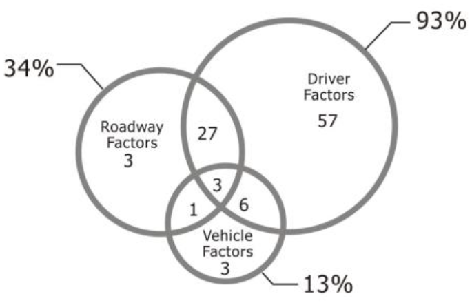
From the American Association of State Highway Transportation Officials ( 5 ).
A basic requirement of HF professionals is to understand both the system and its users. In the context of highways, it is a descriptive term representing an operator’s attempt to perform multiple tasks, often at the same time, when each of the tasks is a cognitive and competitive interference. The operator must fully understand how the system operates and how all the tasks must perform together efficiently and safely. WL is used as a surrogate measure of HF.
For the highway system, we know that earthwork cuts and balances are good for project construction economics. But when done incorrectly, the continuous changing of horizontal and vertical profiles may introduce too many short horizontal curves, tangents, grades, and vertical curves which then diminish user performance and road safety. Roads should be “self-explaining” and be designed to minimize the changing of grades and vertical curves so users expect downstream grades to be similar to upstream rather than a set of random experiences ( 5 , p. 17–11). From an HF perspective these are legitimate issues. Many older two-lane roads appear to need improvements and are often referred to as pioneer trails with high crash rates. In short, it is questionable how well we really understand how users relate to the design and operation of the highway system from an HF perspective.
Highway engineers use policies as the key to successful design, operation, and safe performance of road geometrics and traffic control systems. But this approach, at times, ignores the incorporation and practice of HF principles which can cause unintentional safety problems between the infrastructure and the user.
Workload Principles
An associate key to understanding HF is to understand user workload (WL). When operators are overworked the performance suffers from errors, and when they are underworked they may become complacent. The NASA Primer (Figure 1) shows a WL gauge where 2 to 8 represent the range of acceptable performance ( 6 , p. 2). Unfortunately there is no off-the-shelf gauge available that can be bought. The challenge is to measure WL in a logical, useful way even for highway applications.
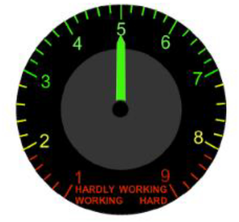
Workload gauge ( 6 ).
The HF literature has numerous examples of the difficulty of defining and measuring WL. In 1990 Hart and Wickens ( 7 ) wrote “operator WL is an important factor that must be considered in evaluating the adequacy and feasibility of operational requirements, system designs, and training procedures” (p. 257). Messer’s ( 8 ) WL definition is “the time rate at which drivers must perform a given amount of work or driving tasks” (p. 7). Senders’ ( 9 ) WL definition is “a measure of the ‘effort’ expended by a human operator while performing a task, independently of the performance of the task itself.” Hamilton et al. ( 10 , p. 10) defined WL as “the total attentional demand placed on the operators as they perform mission tasks.” The difficulty often lies in the relationship between system, operator, and overall performance. No single, overall definition of WL is available.
There are different kinds of WL measures: a) performance; b) indirect; c) subjective; and d) physiological ( 6 , p. 3). Performance measures consider the time it takes to accurately perform several tasks. Indirect measures are used when multiple tasks are performed at the same time to assess how well the secondary tasks are performed after the primary time. In short, is there sufficient time for the secondary tasks to be correctly performed? Subjective measures are the operators’ feelings about the task, that is, whether they are easy or difficult on a subjective scale. Physiological measures include heart rate, heart rate variability, and GSI (galvanic skin response). Each requires special measurement equipment. These types of WL measures are mostly of interest to HF specialists and researchers but not highway engineers.
However, there are two types of WL application that are of value to highway engineers: WL as predictive and/or evaluation tasks. Predictive WL applications would be used during design tasks and evaluation WL would be used for assessing existing roadways. These will be discussed later in the example.
HF Research for Highway Applications
The use of HF for highway applications has been limited because it was not clear what the tasks entailed and because of perceived difficulty in obtaining their quantification. And HF professionals have not yet bridged the void. The following references describe some of the WL research on highway user HF. Some HF researchers have used time-consuming, scientific equipment, that is, eye tracking, heart rate, and galvanic skin response (GSR) equipment connected to computers to gather user response data on how they interfaced with the road environment. For practicing highway designers and traffic engineers, this type of equipment discourages their interest in HF and WL research on road geometrics and traffic control. Significant, leading WL research for practical application is described below.
Messer ( 8 ) in 1980 developed a procedure for quantifying WL by having a group of 21 knowledgeable highway designers and traffic engineers rate 10 geometric features on a subjective scale of 0 to 6 (p. 8). Hamilton et al. ( 10 ) used a subjective analysis of operator task analysis of WL in Army helicopters but on a scale of 1 to 7 (p. 5).
In 1981, Messer et al. ( 11 ) described in further detail the application of Messer’s ( 8 ) procedure for computing WL for two-lane roads. The procedure uses 10 design elements along with Messer’s subjective scale to determine the WL, by road segments. Their final step assigned six levels of consistency (A–F) for each analyzed road segment. ( 11 , p. 41).
In 1992, Krammes and Glascock ( 12 ) published a good discussion of the relationship of various highway design and driver interactions to user WL (p. 1). Their focus was broad and included: road-vehicle-user design and speed inconsistencies, driver expectancy violations, European practices on tangent length and maximum change in degree of curvature, and Australia’s geometric policy for low-speed roads. They described Messer et al.’s ( 11 ) WL-type equation for assessing the change in geometric features from location “n−1” to “n” (p. 44). Five metrics were used in calculating the HF of each feature based on the Messer et al. ( 11 ) subjective and numerical scale from 0 to 6 (p. 8). They focused on identifying geometric inconsistencies based on operating speed changes, and not WL as measured by HF professionals. Krammes and Glascock ( 12 ) state that “.….conceptually, WL is a more appealing basis for quantifying inconsistencies, because it represents the demands placed on the driver by the roadway; operating speed is only one of the observable outputs of the driving task” (p. 4).
In 1995, Fitzpatrick et al. ( 13 ) authored an excellent report on alternative design consistency rating for two-lane highways. They examined speed distribution methods, driver WL of information processing imposed by the road geometrics, and user vision occlusion while driving on two-lane roads. They found many useful attributes on road consistency: the ratio of curve radius to average radius is a sensitive metric for crashes; speed variance is inappropriate for assessing design consistency; WL has good potential for design consistency rating; and user vision demand (VD) is a primary metric within the first 30 m of a curve entrance.
In 2003, NCHRP published Report 488 on driver information overload (DIO) ( 14 , p. 11). The report focused on developing a practical tool or safety model on the relationship of freeway signage and DIO. Their introduction presented a good discussion of how user information overload was broader than signs and that it must include a baseline of the system geometrics DIO. Report 488 reviewed a Positive Guidance analogy but found it not usable as a model to meet their expectation ( 15 , p. 17). Report 488 develops a model with two parts: a “roadway baseline demand”; and a “maneuver proximity” for their freeway signage model ( 14 , p. 13).
Bongiorno et al. ( 16 ) evaluated three drivers in 2017, using GSR to quantify their WL over an 11-km two-lane road in Italy (p. 6). They focused features that were static (curve direction, parked vehicles, and signage) and dynamic (pedestrians, vehicles, motorcycles, and bicycles moving in the same and opposite directions) ( 16 , p. 7). They concluded that user WL was less for fixed features than moving objects because their movements were unpredictable and required continuous monitoring. While the drivers had similar static WL, their dynamic WL was very different.
PIARC published a report in 2019 which identified many European user–infrastructure safety problems ( 4 , p. 40). PIARC has also published many good reports on roadway design standards and HF (visit http://www.piarc.org).
Tignor applied his earlier AR approach (1974 and 2019) when analyzing Snake Hill Road (SHR) by creating a simple baseline “inventory of road features” that users depend on when driving ( 17 ). His approach incorporates a temporal metric in the procedure that measures the renewal time between observed reoccurring events in traveling the road, that is, the time from the start of one horizontal curve to the start of the next curve ( 18 ). This and other metrics are attractive because road users readily make decisions based on time rather than distance (like pedestrian count-down signals). When used with crash data and analyzed with the IHSDM, this method is particularly useful in helping to detect, identify, and explain “potential error locations” having difficult conditions ( 19 ).
DDSA Example Quantification of User–Infrastructure Metrics
The purpose of this simplified example is to illustrate how WL can be used by highway designers and traffic engineers at a fraction of the time and cost of a more formal contract. There are several unique approaches imbedded in the analysis to help understand user WL demands:
quantified “static WL” baseline or inventory of the infrastructure and traffic control features as described by Bongiorno et al. ( 16 , p. 7);
the use of “temporal” metrics;
the AR of geometric design and traffic control elements of the infrastructure (AR of the (a) tangents and curves and (b) grades and vertical curves quantifies the time-length and variance of these elements and they could have a big impact on user WL);
“dynamic WL (DWL)” metrics include lane changes, passing maneuvers, frequency of driveway exiting and entering maneuvers, platoon size, queue waiting time, and so forth;
identification of when predictive and evaluation metrics can be used for assessing user WL;
road designers, traffic engineers, and maintenance staff always serving as a “virtual user” (VU). A VU interacts with the road geometrics and traffic control as if they were a first-time traveler and detects “problematic issues” that should be modified and removed before system implementation.
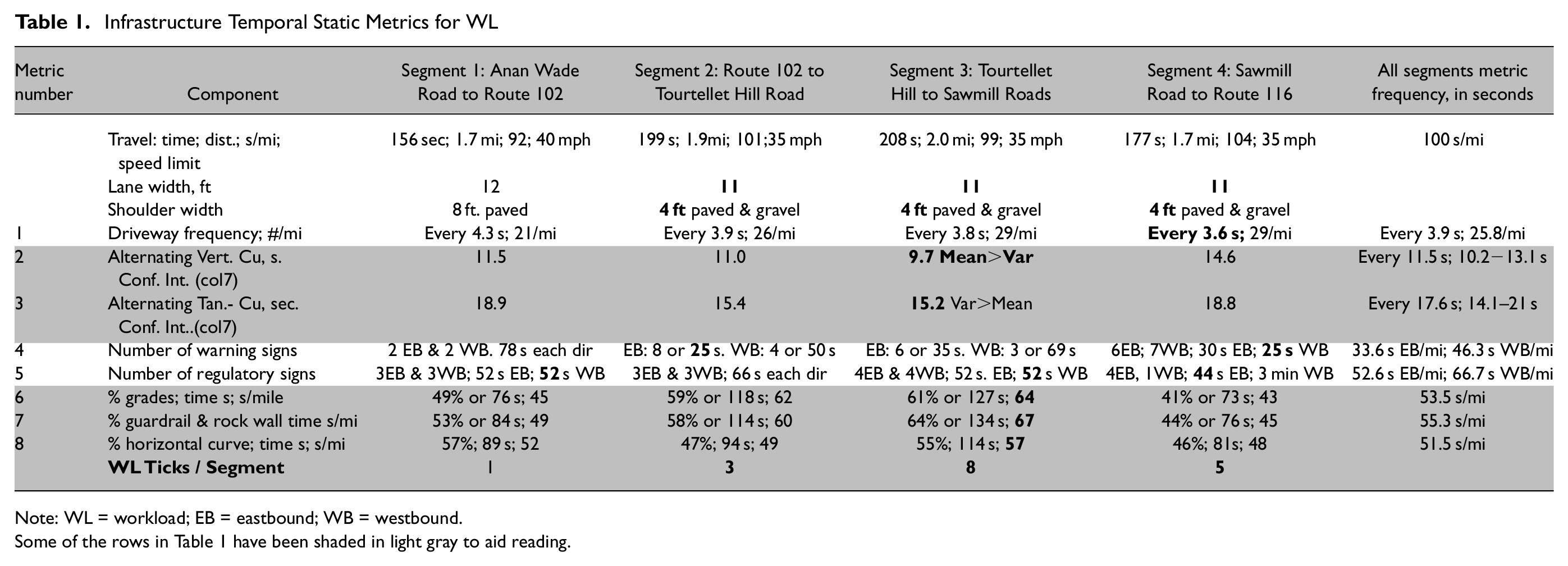
The example is SHR, a 7.4-mi, two-lane suburban-rural type road within 10 mi of an urban area ( 18 ). The road is now more than 40 years old. Originally the design policies were different; the traffic demand and adjoining property have since changed. There is now greater roadside development and the driveway density is 21 to 29 per mile. The route is divided into four segments (see Table 1) with the western end having 12-ft lanes and 8-ft shoulders and three eastern sections have 11-ft lanes and 4-ft shoulders. The route can be reviewed on Google Earth between (41.87175, −71.70791) and (41.86356o, −71.57595o). Each segment was examined and its metrics defined, inventoried, and quantified on exposure time and frequency. Collectively Table 1 identifies eight “static WL” metrics where the last row is a count of “ticks” or numbers (shown in bold) of the critical WL metrics by segment.
Infrastructure Temporal Static Metrics for WL
Note: WL = workload; EB = eastbound; WB = westbound.
Some of the rows in Table 1 have been shaded in light gray to aid reading.
These metrics quantify the temporal frequency infrastructure demands placed on road users by the road designers. They are fixed parts of the infrastructure which users must interact with and respond to when driving as described by Bongiorno et al. ( 16 ).
Metrics include time between driveways, curve and tangent AR times, horizontal and vertical curve AR times, time spacing of warning and regulator signs by direction, percent grades and grade travel time, percent next to guardrail and rock fences and associated travel time, and percent horizontal curve and travel time. These elements are the “static” part of the user WL and attention demand.
A key metric of Table 1 is that the AR of the (a) tangents and curves and (b) grades and vertical curves quantifies the time-length and variance of these elements and they may have a big impact on user safety. AR are especially useful as predictive or evaluation measures of user WL for comparing existing and competing designs.
For the entire SHR, the last column in Table 1, shows the eight time-based metric values. Segment 3 has the greatest number, 8, of temporal metrics. Segment 4 is the second highest largely because of the high number of driveways. The three metrics having the most WL ticks are driveways (averaging every 3.9 s), alternating vertical curves and grades (averaging every 11 s), and alternating horizontal curves and tangents (averaging every 17 s). For SHR the other metrics do not occur as frequently but that does not minimize their importance to road users in making vehicle guidance and control decisions. The WL ticks permit the designers and traffic engineers to compare the consistency of the segments from the perspective of a VU. This avoids the seemingly endless crash modeling and prediction of horizontal and vertical geometrics.
With Table 1 metrics, a designer has a “predictive measure” of user WL for new projects. Also, Table 1 statistics can be used as “evaluation measures” to assess before and after alternative design and traffic control changes.
Figure 2 shows all the static infrastructure metric elements visually present to users. Other roads may have more or fewer infrastructure elements for a WL baseline. Such infrastructure WL baselines can help designers, planners, and traffic engineers (serving as VU) quantify what users experience. Reviewing these metrics by segments aids designers in assessing the magnitude of user attention or WL changes along the road. There has long been a lack of understanding of the interaction between road users and road infrastructure but the metrics used in this example serve to show how infrastructure elements can be quantified as part of user WL. Driveways are included as a metric because of the traffic flow disturbance of vehicles entering and leaving SHR.
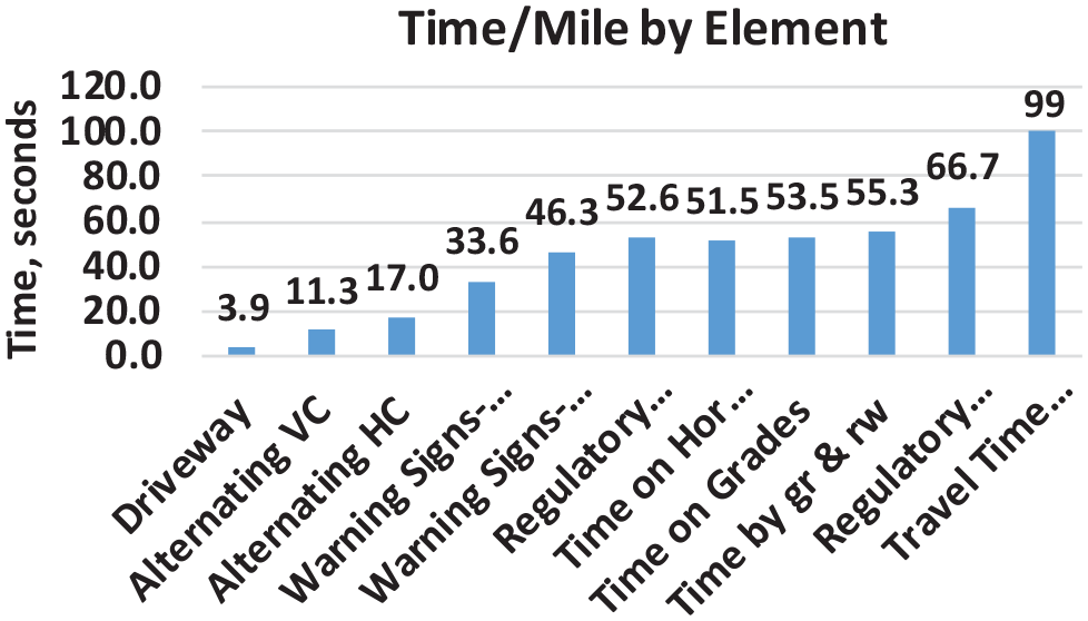
Times for static metrics.
Figure 3 shows for SHR the variation in grade-vertical curve renewal lengths users must continuously interact with the infrastructure. The red circles identify short renewals among longer ones where users must respond to frequent temporal changes in the vertical profile thus requiring a large amount of user WL attention and vehicle conrol. The dashed line is the average grade renewal, 11.5 s. The minimum renewal is 3.3 s and 25% are less than 7.2 s. The black arrow shows the approximate locations of several crashes. The distribution has a normal type shape.

Renewal times for alternating grades and vertical curves.
The renewals of tangents and curves (not shown) are similar with an average of 17.1 s and 30% less than 10 s. But the distribution has a positive skew (many short renewals).
According to Messer ( 8 ), “drivers tend to build up an expectation of what the upcoming roadway is based on during their upstream driving experiences,” a condition for both vertical and horizontal alignments (p. 9).
Table 1 includes warning and regulatory sign metrics because they alert users to different downstream road conditions. Segment 4 had the most warning and regulatory signs but reviews on Google Earth of the roadway geometrics suggested signage was often absent. The amount of time on vertical and horizontal alignment is a measure of user WL and changing conditions that users continuously evaluate and interact with. In this example, guard rails and low rock fences are near the shoulder and users can visually detect them as items that could be a safety impediment should emergency travel path changes be required. Both are more prominent in Segments 3 and 4. Compound vertical and horizontal curves were few (two or fewer in Segments 1 and 2) so they were not used as a metric even though they could be. A passing section metric was not used since SHR had only two short locations in Segment 4.
Messer et al. ( 11 ) reported that a horizontal curvature with a degree of curve (D) greater than 8 significantly increases crash rates. SHR had 12 of 47 curves with a D exceeding 8 (p. 18).
Fitzpatrick ( 13 ) studied VD, “the percent time a driver observes the road,” and found it to be significantly higher on low-radii curves. Ten of the SHR’s 43 had a VD greater than 0.50. Segment 3 had two adjacent curves with a large 59% VD differential. According to Messer et al. ( 11 ) such differentials would challenge driver expectancy and safety (p.10).
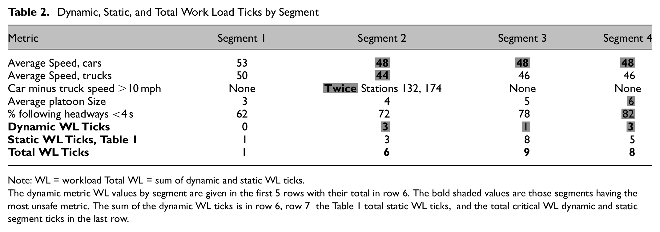
Dynamic WL includes lane changes, vehicle following, passing, pedestrian crossings, signalized traffic control, platoon size, percent vehicles following, and so forth. A limited review of dynamic WL was prepared using the Traffic Analysis Module (TAM) of IHSDM ( 19 ). Only two short sections of SHR permitted passing (Segment 4). Table 2 shows that the average platoon size was 3 or greater and vehicle speeds were reduced in Segments 2 to 4. Segments 3 and 4 had a high percentage of vehicles following, likely because of the greater density of driveway residences. The high percentage platoon following among the segments is indicative of inconsistent design with unstable flow and reduced user safety. The use of mini safety roundabouts (RAB) in these segments may help create larger gaps in the through traffic, smaller platoons, and a reduction of crashes (rear-end and turning).
Dynamic, Static, and Total Work Load Ticks by Segment
Note: WL = workload Total WL = sum of dynamic and static WL ticks.
The dynamic metric WL values by segment are given in the first 5 rows with their total in row 6. The bold shaded values are those segments having the most unsafe metric. The sum of the dynamic WL ticks is in row 6, row 7 the Table 1 total static WL ticks, and the total critical WL dynamic and static segment ticks in the last row.
In accordance with Fitzpatrick et al. ( 13 ), Table 2 shows reasonable consistency in the average speed difference between cars and trucks—2 to 4 mph—across all segments of SHR using TAM (p. 34). However, Segment 2 had two locations with two occurrencs of trucks traveling 13 to 15 mph slower, an unsafe condition according to Messer ( 8 , p. 10). Additionally, Table 2 combines the dynamic and static WL giving the total WL by segments. Segments 3 and 4 were similar in total WL (9 and 8, respecitvely), with Segment 2 closely behind. Note that “Total WL Ticks” is the number of the critical HF metrics found by segment.
Estimation of Potential User–Infrastructure Errors
The geometric design analysis tool IHSDM has five modules that can be used to assess how well a candidate roadway meets current roadway policy ( 19 ). The modules are for: design/speed consistency (DCM); policy review (PRM); traffic analysis (TAM); crash prediction (CPM); and driver-vehicle (DVM). When run, these modules have hundreds of station outputs for each module. IHSDM uses the 2011 AASHTO Geometric Design Policy in PRM evaluations ( 20 ).
IHSDM DCM and PRM modules have primarily been used by practitioners for assessing design consistency and speed even though Krammes and Glascock ( 12 ) state that “.….conceptually, HF is a more appealing basis for quantifying inconsistencies.….” (p. 4).
Figure 4 shows results for DVM and PRM. The DVM dynamic outputs of speed, lateral acceleration, rollover index, and lateral position, provide insight into crash potential and location. The PRM (Figure 4) shows, by segments, results for stopping distance and curve radii for the number of computations meeting and not meeting the required 2011 AASHTO policy ( 20 ). The DVM results indicate similar performance in each of the segments, but Segments 1 to 3 had stopping sight distance (SSD) problems for both horizontal and vertical profiles. Curve radii policy failures were found in Segments 2 and 3. The total PRM problems by segment were 15, 42, 27, and 4 in Segments 1 to 4, respectively.
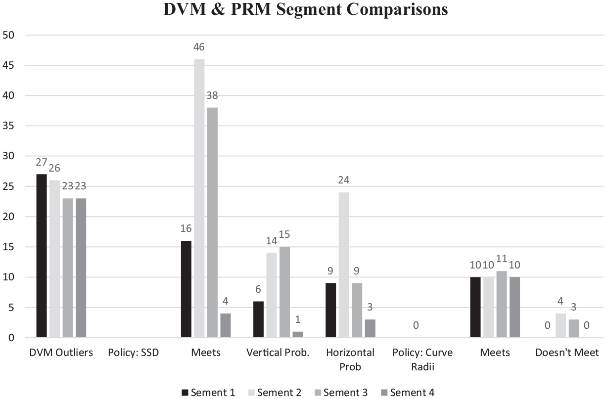
Snake Hill Road: Interactive Highway Safety Design Model results for driver-vehicle and policy review modules (DVM and PRM).
Figure 5, for Segment 2, illustrates by colored flags the locations of IHSDM DVM metrics (rollover, lateral offset, lateral acceleration, curve radii, 85 percentile speed, and 1st & 2nd high crash locations). The general location where road crashes occurred is represented by yellow ellipses. It is striking how the kinematic metrics and actual crashes match so closely.
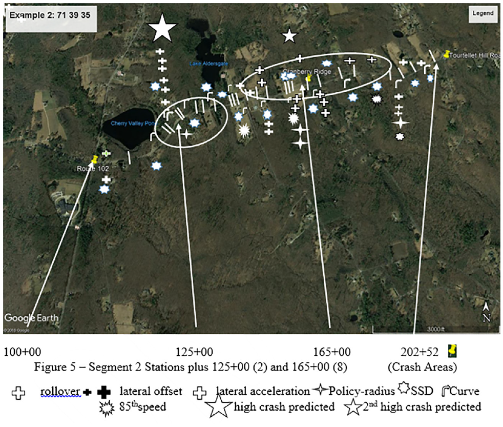
Location of Segment 2: Interactive Highway Safety Design Model flags and real crash locations.
Crashes
Probably the most used investigative technique for understanding road crashes is the police crash report. But police are not trained as highway designers or traffic engineers and the crash reports may be weak in identifying the real cause of errors, especially those involving the interaction between the roadway and users. Also, some crashes occur that are unknown to police because they are never reported. Sometimes, crash evidence remains at the site in the form of damage to power poles, signs, or guardrail, and this may be useful to Department of Transportation (DOT) agencies.
Even if crashes are reported, DOT agencies may not realize the crash is a result of user–infrastructure interaction errors and would fail to follow up with corrective action. The author knows of a case where there was a 3–4 in. rut between the pavement edge and the gravel shoulder on a curve, causing the vehicle to cross the median and strike a car traveling in the opposite direction, killing the driver. For 17 years the shoulder has been reviewed and frequently found to have pavement edge ruts, sometimes being 8–10 in. deep, because the shoulder has not been permanently stabilized (paved).
For the SHR project-predicted IHSDM crashes, Figure 6 shows reasonable “total” agreement to actual crash locations across the four road segments during a five-year period (2008–2012) ( 21 ).
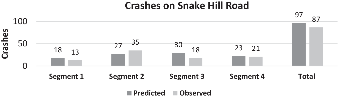
Comparison of predicted and observed crashes on Snake Hill Road.
Road Safety Audits (RSA)
An earlier RSA study for SHR identified problematic safety locations (
21
, p. 23). The interdisciplinary six-person RSA investigated the likelihood of crashes and why crashes may have occurred along the route. The team had available crash data and IHSDM results to help identify and assess potentially complicit infrastructure issues. The team prepared short, intermediate, and long-range safety enhancing recommendations. Their findings were:
HF Guidelines (HFG) and Interaction Matrix (HFIM)
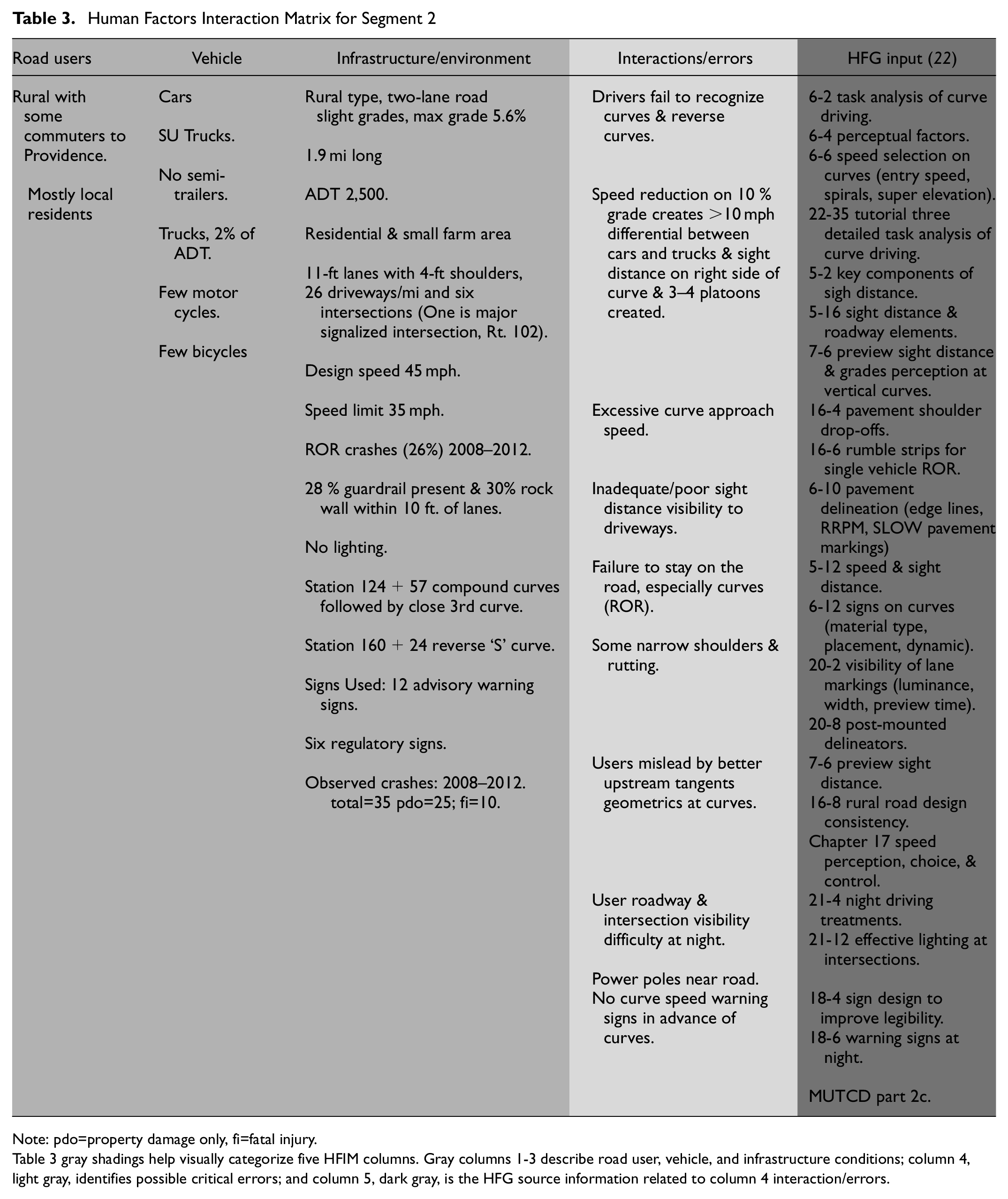
A companion to the HFG is the HFIM, a tool to aid designers and traffic engineers acting as VU to identify potential user–infrastructure errors and solutions ( 22 , 23 ). The HFIM (Table 3) has five columns. The first three columns describe the route’s infrastructure features, vehicle types, and kinds of users. The fourth column (light gray) identifies potential problem interactions between the infrastructure and road user. The fifth column (dark gray) identifies locations within the HFG where highway designer and traffic engineers can obtain help from science-based guidelines addressing problem interactions ( 22 , 23 ). Designers and traffic engineers, as VU, can consider candidate improvements when using the HFG, HFIM, and IHSDM together. Table 3 is the HFIM for SHR, Segment 2. Column 4 is the most important because it identifies eight potential types of HF system errors.
Human Factors Interaction Matrix for Segment 2
Note: pdo=property damage only, fi=fatal injury.
Table 3 gray shadings help visually categorize five HFIM columns. Gray columns 1-3 describe road user, vehicle, and infrastructure conditions; column 4, light gray, identifies possible critical errors; and column 5, dark gray, is the HFG source information related to column 4 interaction/errors.
Table 3 identifies eight potential HF user–infrastructure errors that should be reviewed by the state DOT relative to user safety and operations. These eight potential errors complement the previously discussed findings and the suggested HFG guidelines should be reviewed for each issue.
Recommendations
These recommendations are the result of this DDSA based on use of the unique application of HF and WL analyses. Because SHR Segment 1 has better geometrics and terrain and is less affected by traffic growth, example recommendations are for Segments 2 to 4. Each of the following recommendations includes reasons as why road designers or traffic engineers, serving as a VU, would make their selection. Each recommendation is accompanied by consideration of a combination of: the DDSA analysis; the potential HF user–infrastructure errors; current road policy; Google Earth; HFG; and HFIM.
Lane and shoulder widths should be increased to a newer AASHTO policy which promotes “….operational efficiency, comfort, safety, convenience.” SHR now has narrower lane and shoulder widths ( 20 ).
Power poles and rock walls should be moved away from the thru lanes and shoulder to be in conformance with current AASHTO clear zones. Some are close to the edge of the current shoulder which creates an unnecessary SHR safety hazard ( 24 ).
To enhance driver expectancy, a temporal review of AR of horizontal curve-tangents and vertical grade-curves is needed with more WL uniformity, based on Table 1. Users base their control decisions on upstream knowledge and travel time ( 8 , p. 9).
Damaged guardrail and breakaway cable terminal (BCT) end terminals need replacing to current AASHTO policy ( 24 ). Research shows that 1970-era BCT guardrail end terminals can cause server injury to vehicle occupants. Various new energy absorbing terminals decelerate vehicles with improved performance ( 25 ).
Slow speeds on 10% grade (station 132) needs grade reduction and/or speed warning signs ( 26 ). Table 2 shows two occurrencs when trucks traveled 13 to 15 mph slower; an unsafe HF condition described by Messer ( 8 , p. 10).
To reduce platooning, driveway separations of 4 s or less and minor intersections should be reviewed for use of mini-RABs. Table 1 shows that average driveway time spacing is very close and is thought by the DOT to be associated with traffic flow turbulence and crashes. RABs can modify stream flows and it may be a possible way to create some larger gaps in the flow ( 27 ).
In Segments 2 and 3, VD at curves for driver HF expectancy and sight distance find that safety limitations should be reviewed. Ten of the SHR’s 43 curves had a VD greater than 50%. Segment 3 had two adjacent curves with a large 59% VD differential ( 11 , p. 10).
Some intersections and curves have no advance warning signs for hidden minor roads and curves (user-speed hazards Table 3). The HFG and MUTCD should be consulted ( 22 , 26 ).
Parts of SHR have changing geometrics, many driveways, and minor intersections which may have user nighttime visibility difficulties (see Table 3). A review of nighttime crash occurrences is encouraged to assess the adequacy of user visibility at night ( 22 ).
Conclusions
This paper illustrates the importance of recognizing, quantifying, and understanding the interaction of user HF and roadway infrastructure. Review of published reports suggests that user HF is a viable and strong focus when assessing highway geometrics and user safety, and “….driver HF values may be good predictors of accident experience on two-lane rural highways” ( 12 , p. 9). Following the discussion of HF research, a simple approach is presented for analyzing two-lane roads using WL to quantify user tasks. This candidate analysis approach can be used by designers and traffic engineers for either prediction or evaluation in HF safety analyses.
The use of eight static and four dynamic metrics illustrates for a 7.6-mi. two-lane suburban/rural road example how user HFs are challenged with the road infrastructure. The fixed static WL metrics were: driveways, alternating horizontal curves, alternating vertical curves, warning and guide signs, grades, rock walls, and curve time. The traffic DWL metrics were: average car and truck speeds, car–truck speed differentials of more than 10 mph, platoon size, and percentage of following platoons. Vehicle kinematic metrics (rollover, lateral offset, lateral acceleration) and AASHTO policy design consistency metrics (curve radii and stopping sight issues) were included in the HF analysis. Google Earth, Excel, and IHSDM were the analysis tools. Use of “temporal” metrics, VU attention, and AR of geometric design and traffic control elements of the infrastructure were key ranking metrics for user WL demands. HFIM and HFG supported development of findings and recommendations.
The Total HF analysis, Table 2, convincingly showed that, in the four segments, users experienced different types of WL. Segment 1, because of its uniform terrain and higher design, had the lowest level of WL at 1. Segment 2’s total WL was 6. Segments 3 and 4 had similar levels of WL ( 8 , 9 ), but the static WL was the highest in Segment 3 because: a) the shorter AR of vertical and horizontal curve times creates greater user–infrastructure demand; and b) the D of adjacent curves differed more than 3° in six locations. For DWL, Segment 4 had the largest average platoon size ( 6 ) and percent following headways (82) less than 4 s.
To summarize, it is recommended that highway designers, planners, and traffic engineers incorporate HF, WL, AR, VU principles, temporal metrics, RSA, HFG, HFIM, IHSDM, and VD as illustrated, in assessing project road safety before implementation. When used together, these tools have a great potential for significant contributions in DDSA ( 1 ). The HF and WL metrics presented in this paper would be appropriate for integration into road design software.
Footnotes
Acknowledgements
This report is a DDSA expansion of the July 2014 report FHWA-SA-14-071 by Nabors, Dan, and Goughnour, Elissa, “Road Safety Audit Case Studies: Using IHSDM in the RSA Process.” Special thanks go to Sean Raymond (RIDOT), Elissa Goughnour (VHB), Mohamad Banihasemi (formerly with CYFOR Technologies LLC, now with FHWA), and Mike Dimaiuta (Genex Systems), Jerry Roche and Jeff Shaw (FHWA), and Dr. John L. Campbell (Exponent) for their input, technical reviews, suggestions, and thanks to Dr. Rick Pain (retired TRB) for discussions and encouragement.
Declaration of Conflicting Interests
The author declared no potential conflicts of interest with respect to the research, authorship, and/or publication of this article.
Funding
The author received no financial support for the research, authorship, and/or publication of this article.