Developing a Google Earth-Based Method to Measure Sight Distance for U-Turns at Unsignalized Intersections on Multilane Divided Highways

Abstract

The median U-turn is one of the most popular access management techniques implemented by state transportation agencies. Sight distance (SD) is among the key elements for the safe operation of median U-turns. The traditional method of measuring SD is using sight rods in the field, which is inconvenient and unsafe; thus, it is important to develop a convenient and safer method to measure SD for U-turn movement. The objective of this study is to develop a safe and cost-effective method to measure SD for U-turn vehicles, without going into the field, using existing tools in Google Earth and a perspective grid method that can be generated by Kinovea software. The method can be used in two different road geometric conditions: (i) a straight segment with crest curves; (ii) a roadway with a combination of crest curves and horizontal curves. For Condition (i), an empirical equation was developed to estimate SD as a function of distance and elevation along the sight line measured using Google Earth. For Condition (ii), a perspective grid was first applied using Google Earth ground-level view; then the number of broken lines and gaps in each perspective grid cell was used to measure the SD. All inputs can be collected using Google Earth. Field measurements of SD for U-turns at 10 selected locations were conducted to verify the validity of the method. The results show that the differences between the model estimates and field measurements are all less than 10%.

Keywords

Infrastructure roadway design performance effects of geometric design sign distance (SD)stopping SSD intersection SD decision DSD,etc.operations;access management u turn

As restricted crossing U-turn intersections are increasingly implemented on multilane rural divided highways, more U-turn traffic movements occur at these unsignalized intersections. According to the median U-turn intersection design guide by the Federal Highway Administration (FHWA), designers should ensure a good intersection sight distance (SD) at median U-turn crossovers by ensuring slopes and plantings in the median are cut back beyond the lines of sight ( 1 ). An ongoing research project on the safety of unsignalized intersections on rural multilane divided highways funded by the Alabama Department of Transportation found that some median openings experience an alarmingly high number of U-turn-related crashes. A field review of the high-crash locations revealed that some of these locations have limited SD for U-turn drivers. The research team selected a three-mile roadway segment to study the crash history of U-turn movements at unsignalized intersections. Based on crash data collected from the Critical Analysis Reporting Environment (CARE) database (2), there were a total of 70 crashes from 2009 to 2014 on this three-mile segment with 10 median openings from the milepost 74 to 77 on U.S. 280 in Alabama; 54% of which happened on the one-mile segment between the milepost 74.5 to 75.5, where the three median openings had very short SD. Crash data analysis found that approximately 30% of total crashes on this one-mile segment were U-turn related, resulting in one incapacitating injury, seven non-incapacitating injuries, and eight property damage only crashes. Insufficient SD for U-turns might be an important contributing factor. In this study, the researchers first measured the SD for U-turns at the 10 median openings on U.S. 280 in Alabama from milepost 74 to 77. U.S. 280 is a high-speed multilane divided highway with a wide median. Field observations and measurements suggested that SD is strongly correlated with terrain, elevation, grade change, vertical curves, and horizontal curves. Figure 1 shows the top view and elevation profile of the three-mile study segment on U.S. 280.

Figure 1.

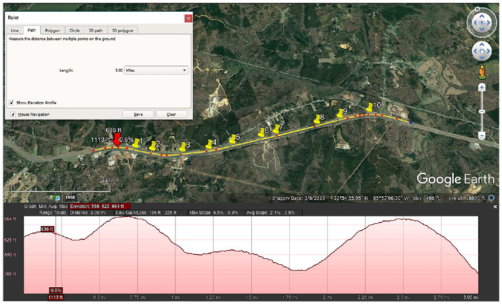
Top view and elevation profile of case study segment.

The traditional SD measurement method, which uses sighting and target rods in the middle of the road, is extremely dangerous, especially on high-speed rural highways. The main goal of this study is to develop a cost-efficient and safe way to estimate SD for U-turns and to help identify the median openings with restricted SD for U-turns at unsignalized intersections on multilane high-speed roadways. The developed method allows engineers to estimate the U-turn SD in the office using the Google Earth Ground View function, which is different from Google Street View.

Two different methods were developed for two defined conditions: (i) straight roadway segments with crest curves; (ii) roadway segments with a combination of crest curves and horizontal curves. A roadway segment with a sag curve will not create SD issues for U-turns. For Condition (i), an equation was established as a function of distance and elevation to calculate the SDs. Google Earth’s ruler tool can be used to measure the length between two points, the elevation of each point, and the roadway’s elevation profile. For Condition (ii), the perspective grid was used as a supplemental tool for Google Earth. The method includes two steps: (a) apply the perspective grid on top of the ground-level view in Google Earth to separate the road into various same length segments; (b) utilize the broken line marking as a reference length and ruler in Google Earth to estimate the SDs in Google Earth’s ground-level view. The rest of this paper includes a literature review of SD definitions, previous measurement methods, standards for SD for U-turns, methodology development, case studies, and conclusion.

Literature Review

Definition of SD

SD is the length of the roadway ahead that is visible to a driver. According to the Greenbook, 2018 edition ( 3 ), the designer (of a roadway) should provide SD of sufficient length, which will allow drivers to control the operation of their vehicles to avoid striking an unexpected object in the traveled way. Drivers’ SD is also one of the most important factors that influence traffic safety. Note there are three types of SD: stopping SD, decision SD, and intersection SD. A driver’s sight line will be obstructed by the geometric features or objects on roads. On horizontal curves, a driver’s sight will be blocked by trees, signs, buildings, or slopes. On crest curves, a driver’s SD will be decreased when the grade difference increases. During nighttime, the SD of a sag curve will be restricted by vehicle headlights for through movements The sag curve does not create an SD problem for U-turns at the median openings in both the daytime and nighttime.

NCHRP Report 524 states that intersection SD (ISD) is an important safety and operational consideration in the design of a median opening ( 4 ). NCHRP Report 375 states that ISD at median openings is complicated by the presence of the median itself ( 5 ), which may increase the ISD requirements at some locations or may contain sight obstructions that reduce ISD. If a median is wide enough to store a vehicle, the ISD requirements of an intersection can be determined separately for each directional roadway. Insufficient ISD has both safety and operational problems at the intersection. From a safety standpoint, drivers with insufficient ISD may be unable to anticipate and avoid potential collisions. From an operational standpoint, drivers with insufficient ISD may either extend their vehicle into the traffic stream to improve their view of the roadway or accept less than desirable gaps in the traffic stream. Either behavior may cause other vehicles to perform evasive or braking maneuvers. A study by the Kentucky Transportation Cabinet and FHWA ( 6 ) found that U-turn design is very effective in reducing the delays and crash rates at stopped controlled median openings; thus, the potential cause of a higher crash rate for a U-turn may be insufficient SD. Other studies on SD include: Awadallah ( 7 ), which developed the guidelines for three types of ISDs (i.e., approach SD, sign visibility SD, and stop-line distance); NCHRP Report 650 ( 8 ), which developed guidelines on SD for median intersection design for rural high-speed divided highways; and Gargoum et al. ( 9 ), which pointed out that different age groups have different requirements for SD. None of these studies, however, provide standard SDs for U-turn movements.

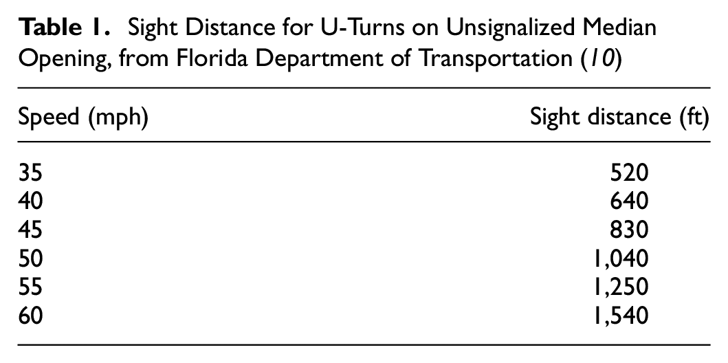
There is also no standard for SD requirements for median openings in the 7th edition of AASHTO Green Book, A Policy on Geometric Design of Highways and Streets ( 3 ). Some state Departments of Transportation have their own design standards or guidelines on the SDs for U-turns. The Florida Median Handbook 2014 defined the ISD at unsignalized intersections for a U-turn movement ( 10 ), as shown in Figure 1. The handbook ( 10 ) also recommended minimum SD values for U-turns at unsignalized median openings for specific speeds (Table 1).

Table 1.

Sight Distance for U-Turns on Unsignalized Median Opening, from Florida Department of Transportation ( 10 )

Speed (mph)	Sight distance (ft)
35	520
40	640
45	830
50	1,040
55	1,250
60	1,540

Figure 2.

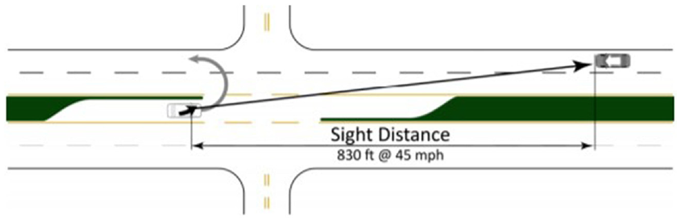
U-turn sight distance, from Florida Department of Transportation ( 10 ).

SD Measurement Methods

The traditional method of measuring SD is to use sighting and target rods in the field ( 11 ). A target rod can be constructed out of lengths of 2 in. by 0.75 in. wood. The target rod should be 4.25 ft high to represent vehicle height and painted fluorescent orange on the top portion and bottom 2 ft of the rod. The bottom 2 ft portion represents the object height for measuring SD. The sighting rod should be 3.5 ft tall to represent the driver’s eye height. The sighting rod can be constructed out of the same type of wood but should be painted flat black, as shown in Figure 3.

Figure 3.

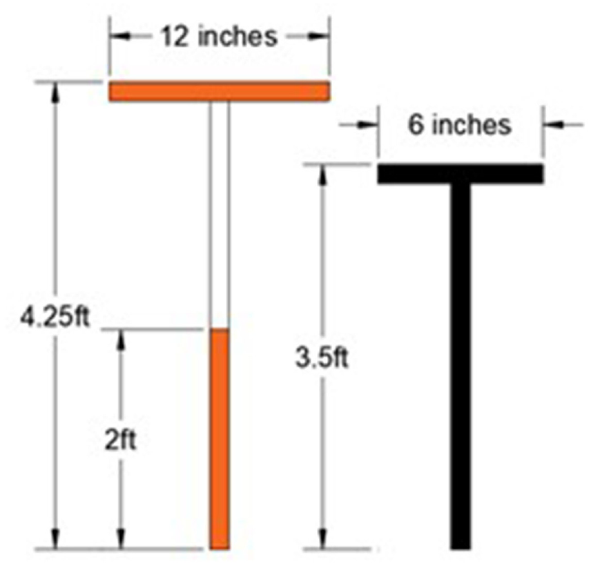
Target rod (left) and sighting rod (right).

Because of the inconvenience of the traditional method, past studies have developed new ways to measure SD. Most recent studies on this subject focused on using geographic information system (GIS) and other sources to establish a formula to calculate SD for existing roads. In 2011, Castro et al. ( 12 ) suggested building a three-dimensional (3D) model by using a digital surface model instead of a digital terrain model to make up for the drawbacks of the design software. The digital terrain model usually ignores the influence of side obstacles, such as trees or buildings, which may significantly reduce drivers’ SD. In 2013, Castro et al. ( 13 ) introduced software to calculate SD supported by GIS and a trajectory defined by points obtained with a global navigation satellite system (GNSS) receiver instead of relying on project information ( 13 ). Another advantage of this software is that it solved how to measure SD on roads whose design information is not available. In 2014, Castro et al. ( 13 ) developed a method to measure the distance of the hidden area of an existing road from georeferenced photographs ( 14 ). This method contains six steps: setting calibration of the digital camera to reduce measurement errors; measuring highway width in the section where distances will be measured; taking photos and registering the camera position with a GNSS receiver; measuring highway width in the photos (in pixels); calculating distances; and calculating the length of the hidden section. After comparing the results with distances measured by GNSS, it was found that the error between these two results was small enough for use in traffic safety studies. In 2017, Jung et al. ( 15 ) investigated a method to measure SD based on high-resolution LiDAR data. This developed method allowed engineers to use a 3D model to evaluate the SD virtually considering a variety of objects, for example, vehicle types, multimodal forms of transportation (bicycle, pedestrian). This model enables the algorithm to successfully evaluate SD constraints from a variety of vehicles, driver heights, and viewing angles as well as multimodal forms of transportation. Since 2018, more studies that have adopted remote sensing techniques, such as using LiDAR to assess stopping and passing SD on highways ( 16 – 19 ). However, all the above methods required expensive software, extensive training, and detailed data on roadways. There is a need to develop a method for transportation practitioners that can estimate SD based on common public accessible tools, such as Google Earth.

Google Earth Pro

Google Earth Pro is a combination of superimposing satellite images ( 20 ), aerial photography, and GIS data onto a 3D globe, allowing users to see cities and landscapes from various angles.

In Google Earth Pro 6 Edition, released in 2011, a ground-level view function in which users can switch from ground view to street view using the button at the upper-right corner in the Google Earth Pro software, and vice versa (see Figure 4) was added to simulate a driver’s sight line just above the ground (Figure 4, left). The ground-level view can provide a new way to see terrain and surroundings that is completely different from Google Street View. In the ground-level view function, a two-dimensional (2D) roadway surface image is provided; this image contains the basic geometric information (such as X, Y coordinates and elevations) at the bottom (Figure 4, left). Another advantage of the ground-level view is that its database is updated more frequently than the Street View database (Figure 4, right). For example, in Figure 4, the ground view’s date is March 2019, and the Street View image at the same location is from April 2017. Besides, the eye height of the ground view is the same as the roadway’s elevation, and it will not be affected by the camera height of the Google van that was used to collect street view images. Furthermore, the driver’s eye height can be set up flexibly, unrestricted by the Google van. The observing location can be moved to any point by scrolling the mouse. The ground views from the center of the road were found to be the best images to apply a perspective grid to estimate the SD. To use the ground-level view function to measure the SD, an additional tool called the “perspective grid” needs to be understood and properly applied. The next paragraph briefly introduces the perspective theory for a better understanding of the perspective grid method.

Figure 4.

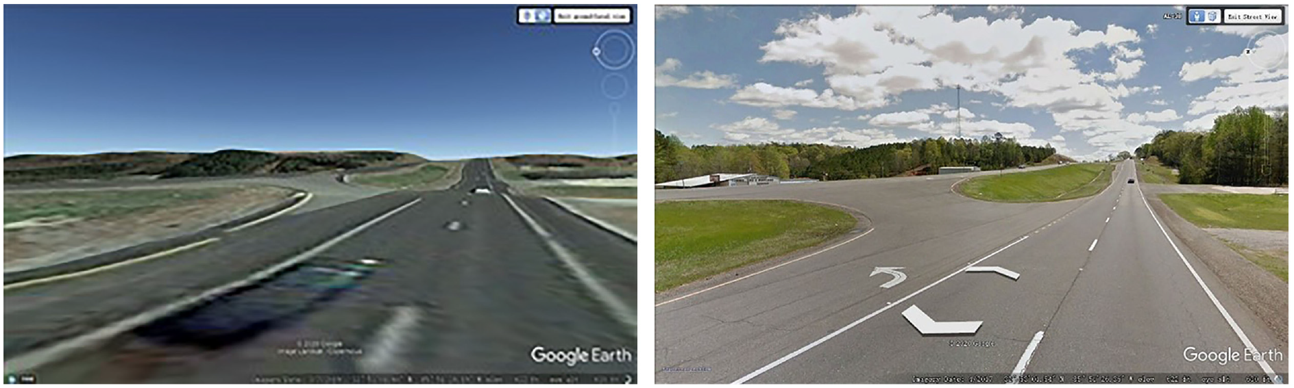
Ground view for March 2019 (left) and street view for April 2017 (right) at the same location.

Perspective Theory

Based on the theory of perspective, objects shown in a 2D picture appear smaller as their distance from the observer increases ( 21 – 25 ). They are subject to foreshortening, meaning that an object’s dimensions along the line of sight appear shorter than its dimensions across the line of sight. When roads or objects are directly faced to the observer, a one-point perspective is suited for this situation. An image has a one-point perspective phenomenon when it contains only one vanishing point on the horizon line. This type of perspective is typically used for images of roads, railway tracks, hallways, or buildings viewed so that the front is directly facing the viewer. Any objects that are made up of lines either directly parallel with the viewer’s line of sight or directly perpendicular (the rails) can be represented with a one-point perspective. These parallel lines converge at the vanishing point. Based on this theory, the perspective grid (which is a network of lines, drawn or superimposed on a photograph, to represent the perspective of a systematic network of lines on the ground or datum plane and can simulate how objects change in the picture) was applied to divide the road into several parts to estimate the actual length of the road in the picture. It can be used to measure the ISD based on a ground-level view image in Google Earth. Figure 5 shows an example of a 5 × 5 perspective grid. The border of the grid represents the border of the road. When applying the perspective grid on the ground-level view, the border of the grid covers the edge lines of the highway. Further, the perspective grid can be divided into n × n depending on different conditions.

Figure 5.

Perspective grid.

Computer vision ( 26 ) is another method that can be used to estimate the actual size through a 2D picture. LiDAR data can also be used to estimate SD ( 27 ). However, these two methods are more complicated and expensive to implement than using the perspective grid on Google Earth ground-view images.

Methodology

In this paper, a Google Earth-based method was developed to help traffic engineers measure SD for U-turns at unsignalized intersections on a divided highway without going to the field or using expensive design software. When the U-turn median openings are located on a flat and straight segment (Figure 6), U-turn drivers typically have sufficient SD because there is no obstacle to affect the sightline. When there is a sag vertical curve, in the daytime, drivers will have sufficient SD; drivers can also see oncoming vehicle headlights at night. Based on the field reviews, it was found that the SD for a U-turn needs to be checked for a safety study under these two conditions: (i) a straight segment with crest curve; (ii) a roadway segment with a combination of crest curve and horizontal curve or horizontal curve only.

Figure 6.

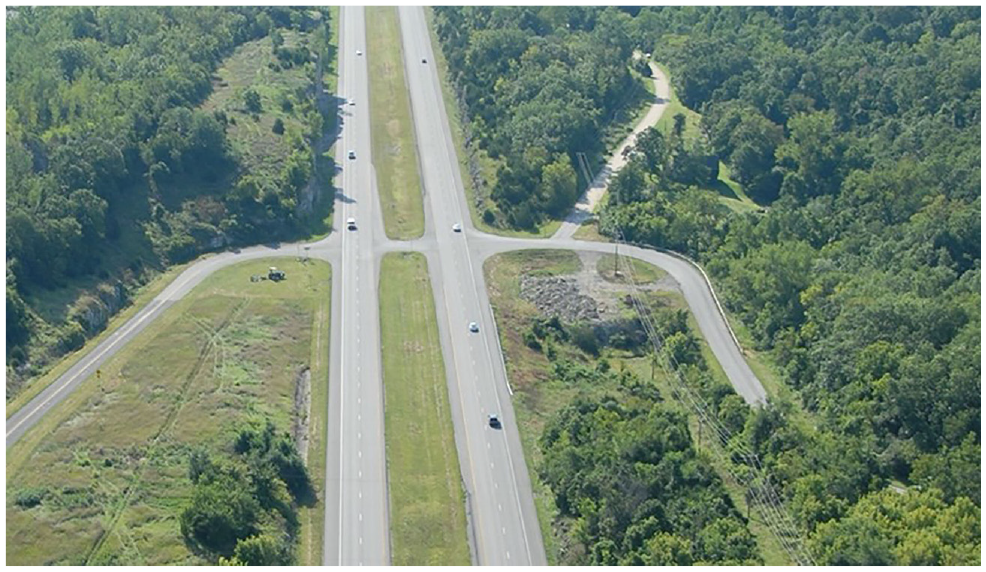
Example of median opening located on a flat and straight segment.

Method to Estimate SD for the Condition i

For Condition (i), the SD for U-turn movements can be estimated as the horizontal distance from Point A to Point B, as shown in Figure 7.

Figure 7.

Sight distance for Condition (i).

The U-turn vehicle’s coordinates are represented as E(X1, Y1), where X1 is the distance from Point E to the highest Point C of the crest curve; Y1 is the elevation of the point where the U-turn vehicle stopped. D(X2, Y2) is the coordinates of the point that can generate a line CD that represents the roadway’s slope, where X2 is the horizontal distance from Point D to Point C; Y2 is the elevation of Point D. C(X0, Y0) is the highest point of the crest curve. Lines EC and CD represent the tangents of the crest vertical curve. In this study, driver’s eye height, $h_{1}$ is assumed as 3.5 ft ( 11 ) and the object’s height $h_{2}$ is assumed as 4.25 ft. Any point’s elevation, $Y_{AC}$ on line AC can be calculated by Equation 1:

Y_{AC} = \frac{Y 1 + h_{1} - Y 0}{X 1} \times X_{a},

(1)

where $X_{a}$ is the horizontal coordinate of any point on line AC.

Any point’s elevation $Y_{CD}$ on line CD can be calculated by Equation 2:

Y_{CD} = \frac{Y 2 - Y 0}{X 2} \times X_{b},

(2)

where $X_{b}$ is the horizontal coordinate of any point on line CD.

As shown in Figure 7, the elevation of Point B on line AC is $h_{2}$ higher than the corresponding point on line CD. Thus, we can obtain Equation 3 by combining Equations 1 and 2:

Y_{AC} = Y_{CD} + h_{2},

(3)

Then, the horizontal coordinate of Point B can be calculated by Equation 4 after simplifying Equation 3:

X_{c} = | \frac{h 2}{(\frac{Y 1 + h 1 - Y 0}{X 1} - \frac{Y 2 - Y 0}{X 2})} |,

(4)

where $X_{c}$ is the horizontal coordinate of Point B, so the equation for SD is Equation 5:

SD = | X_{1} | + Xc .

(5)

Because we do not have the vertical curve design information, it is difficult to find the exact coordinates of the (X0, Y0) in the field. When applying this equation to estimate SD, the highest point of each crest curve was assumed as the point with the highest elevation (X0, Y0), shown in Figure 1, measured in Google Earth. The $X_{2}$ horizontal coordinate for Point D was assumed to be 500 ft to calculate the equation of line CD because 500 ft is long enough to show the crest slope (the CD line is only used as a reference).

In Condition (i), the road can be treated as a straight line without a horizontal curve. Based on Table 1, the U-turn SD was 1,540 ft at 60 mph. The speed limit is 65 mph at case study locations in this project. Thus, the method developed can be applied for any straight segment with a length less than 2,000 ft. Equation 6 can be obtained after inputting the assumed values for estimating the SD for U-turns:

SD = \frac{4.25 \times X_{1} \times X_{2}}{(Y_{1} + 3.5 - Y_{0}) \times X_{2} - (Y_{2} - Y_{0}) \times X_{1}} + | X_{1} |

(6)

Method to Estimate SD for Condition (ii)

For Condition (ii), SD will not only be affected by the vertical curve but also by the horizontal curve. Equation 6 does not suit for Condition (ii) because the highest location that drivers can see will be affected by the horizontal curve. As shown in Figure 8, the small hill blocks the driver’s sight. In this study, a method is proposed to measure the SD by using a perspective grid on a Google Earth ground-level view image of a roadway segment.

Figure 8.

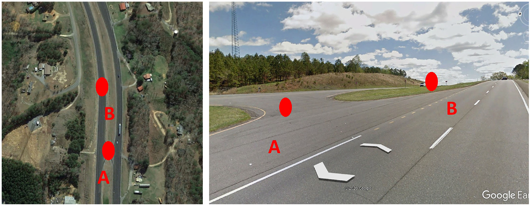
Example location where sight distance is affected by both vertical and horizontal curves.

The reason that the ground-level view was selected is that the ground-level view function allows users to place an observing location at any point, no matter if this point was included in the trajectories of the collecting vehicle for the Street View function. Google Street View can only show the images taken by the data-collecting vehicle.

The ground-level view in Google Earth can be seen as a case of one-point perspective, as shown in Figure 9 (right). To measure the SD on the Google Earth ground-level view image, the perspective grid is recommended for the one-point perspective case to estimate distances in a 2D image, which grid is generated by Kinovea software.

Figure 9.

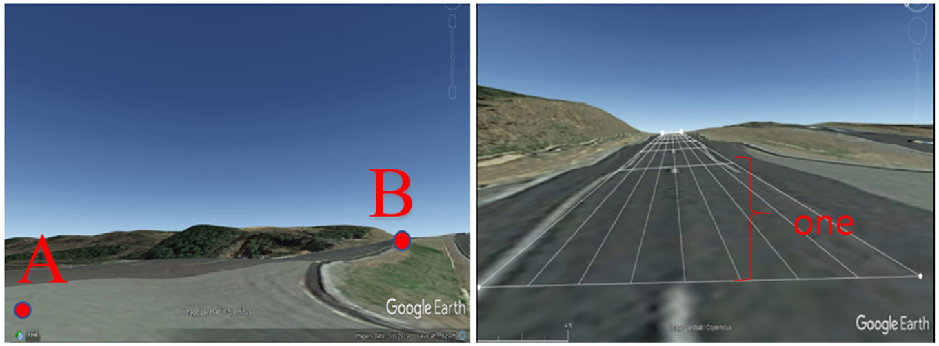
Observing at median opening (left); Observing with perspective theory (right).

In the ground-level view in Figure 9 (left), we can identify the farthest point, B, from the observing point, A. However, without detailed information, such as pixels, resolution, camera focal length, and so forth, it would be impossible to measure the SD directly from the image. In this study, the perspective grid was (generated by Kinovea) selected as a reference tool to help divide the picture into different parts. Each part represents the same distance in the real world. As shown in Figure 9 (left), when the vehicle is stopped at the median, the driver does not directly face oncoming traffic on the road. Thus, it was difficult to find a known object for reference in the figure. To calculate the SD, the next step was to scroll the mouse until the observer directly faced the oncoming traffic on the road, as shown in Figure 9 (right). The perspective grid could then be applied to cover the road surface. In this study, an 8 × 8 perspective grid was used to divide the road into eight parts, as shown in Figure 9 (right). Since each cell represents the same distance, the actual SD can be estimated to be equal to eight times the length of one cell. Users can also use different sizes of the perspective grid to match different situations, for example, a 16 ×16 grid to measure a longer road.

The method described above was only suitable for the case in which there was a crest vertical curve combined with a horizontal curve, and where the highest point of the vertical curve was behind the point of intersection of the horizontal curve because, in this condition, the horizontal curve will have a significant impact on the SD.

Field Data Collection

The developed method was used to estimate SDs at the 10 median openings on U.S. 280 in Alabama from milepost 74 to 77. The SDs estimated by this method were verified by SDs measured in the field.

In this study, researchers did not use the traditional field measurement method because of safety concerns. A three-step alternative method was developed to measure SDs in the field. The first step is to use the GoPro camera as a recording tool to record the driving environment. The GoPro camera can be installed over a driver’s head right above the eye and used to record a driver’s front views. The farthest point seen in the video is close to the farthest point that a driver’s sight line can reach in the field. Second, Google Earth is used to identify an object on the road, for example, a traffic sign or roadside object, as a reference to determine the farthest point in the video. The last step is to use Google Earth to measure the distance between the farthest point in the video and the centerline of the median opening.

To determine the farthest point in a driver’s sightline, a researcher driving a vehicle stopped at the U-turn median opening and observed the vehicles in the opposing direction. When the driver saw the first vehicle appearing in the view at the farthest point, screenshots were taken by GoPro. From these, researchers could estimate the actual vehicle location via Google Earth by using the objects on the roadside as references to obtain the SD. The SDs for U-turns from both directions were measured at the 10 study locations. For each location, two points from each direction were selected as reference points to present the elevation changes. These elevation data were used to estimate SDs in Equations 1 and 2.

Table 2 lists the field-measured SDs and elevation change points for the study median openings. U-1 means the first median opening. For the U-turn SD column, “A (East to West)” represents the SD for the direction from east to west; “B (West to East)” represents the SD for the direction from west to east. In the column “Elevation,”“1st farthest of A” and “U-turn vehicle of A” represent the elevation of the farthest point that the U-turn sight line can reach and vehicle elevation at the median opening for direction “A (East to West),” respectively. “1st farthest of B” and “U-turn vehicle of B” represent the elevation of the farthest point that a U-turn sight line can reach and vehicle elevation at the median opening for direction “B (West to East),” respectively. U-turn SD data were used to identify which road segment belongs to which condition, and elevation data were used in Equations 1 and 2.

Table 2.

Summary of Field Data

	U-turn SD (ft)		Elevation (ft)
	A (East to West)	B (West to East)	1st Farthest (A)	U-turn vehicle (A)	1st Farthest (B)	U-turn vehicle (B)
U-1	1262	938	663	622	653	622
U-2	343	>2000	653	652	663	652
U-3	>2000	412	609	658	671	661
U-4	>2000	1758	635	612	670	608
U-5	1001	>2000	609	605	605	606
U-6	>2000	>2000	604	603	602	576
U-7	>2000	>2000	606	587	587	609
U-8	>2000	>2000	586	610	611	656
U-9	991	>2000	614	650	650	660
U-10	>2000	>2000	660	657	655	643

Note: SD = sight distance.

The data in the “Elevation” columns were collected from elevation profiles of the road to help the researchers identify which road segment belongs to which condition; they were also used in Equation 6 for Condition (i).

Results

Based on the field data analysis, three median openings meet Condition (i): U-1 direction B, U-4 direction B, and U-5 direction A. Five median openings meet Condition (ii): U-1 direction A, U-2 direction A, U-3 direction B, U-7 direction B, and U-9 direction A.

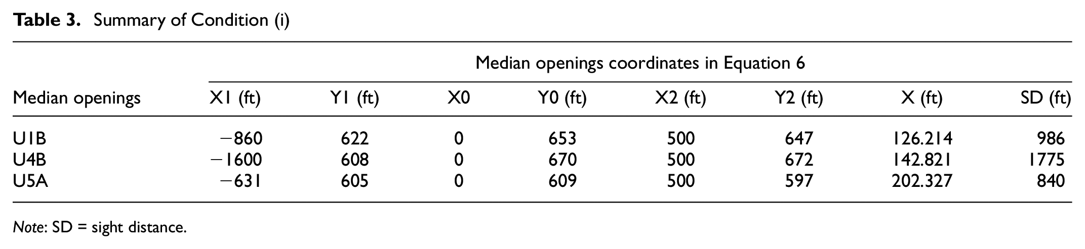
For Condition (i), all necessary input data for Equation 6 are collected, as listed in Table 3. SDs were estimated by Equation 6, as shown in the last column of Table 3. U1B refers to the first median opening for direction B. U4B refers to the fourth median opening for direction B and so on.

Table 3.

Summary of Condition (i)

	Median openings coordinates in Equation 6
Median openings	X1 (ft)	Y1 (ft)	X0	Y0 (ft)	X2 (ft)	Y2 (ft)	X (ft)	SD (ft)
U1B	−860	622	0	653	500	647	126.214	986
U4B	−1600	608	0	670	500	672	142.821	1775
U5A	−631	605	0	609	500	597	202.327	840

Note: SD = sight distance.

For U1B and U5A, the SDs of 986 and 833 ft were significantly less than the 1,540 ft minimum requirement for the speed limit of 60 mph based on the recommendation in Table 1.

For Condition (ii), researchers first used the perspective grid to divide the figure into eight parts and then counted the broken line pavement markings in each cell. Based on manual uniform traffic control devices (MUTCD), a broken line is 10 ft long, and the gap between two broken lines is 30 ft. Figure 9 shows an example of median opening U2A. In Figure 9 (right), one cell length has one broken line and one gap, it is 40 ft, so the estimated distance is 320 ft. This is close to the distance measured in the field (343 ft). Although the length estimated by the perspective grid was the length of the road that is close to the SD, the estimated length of a roadway can be adjusted by the roadway grade. For example, if there is a 3% grade on the divided highway, SD divided by the road length is equal to $\cos (\tan^{- 1} (3 %)) = 0.9995 .$ Applying it to the SD of U2A, the final SD is equal to 320 × 0.9995 = 319.8 $ ft.

Table 4 lists a summary of all the estimated SDs and field-measured SDs at seven median openings for both conditions. The percentage of the difference between field and estimation data ranges from 7% to only 1%. Roadway conditions for the study sites U6, U8, and U10 do not meet the defined conditions so no SDs were estimated for these three locations.

Table 4.

Summary of Field-Measured and Estimated Sight Distances

	Median openings
	U1A	U1B	U2A	U3B	U4B	U5A	U7B	U9A
Field (ft)	1262	938	343	412	1758	901	2153	991
Estimation (ft)	1280	986	320	397	1775	840	2139	1020
Difference (%)	1	5	−7	−4	1	−7	−1	3

Conclusion

In this study, a method is developed to measure the SD for U-turns at unsignalized intersections for two geometric road conditions: (i) a straight segment with crest curves; and (ii) a roadway segment with a combination of crest curve and horizontal curve. By using this method, traffic engineers do not have to go to the field to measure the SDs. The estimated SDs for seven locations that meet the two defined road conditions were compared with the field-measured SDs.

For Condition (i), because the highest point on the crest curve was assumed to be the tangent point of the sight line and crest curve, this will cause SD to be overestimated by Equation 6, so the difference between model and field was positive. For Condition (ii), when researchers applied the perspective grid to the ground-level view, the starting point was the first broken line shown in the view, so the measurements will be a little shorter than the real SD, thus, the difference between method measurements and field measurements was negative.

Limitations

This method cannot be proposed as a replacement to a more rigorous assessment of SD. One of the major limitations of the proposed method is the subjectivity in many of the proposed steps, for example: (a) scrolling the mouse until the observer directly faces oncoming traffic; (b) picking the highest point of verticle curves; (c) counting broken line pavement markings. This method is only intended as a preliminary assessment.

Other factors may also affect the accuracy of SD estimation, such as the procedure of estimating SD using GoPro videos. Further, the elevation of selected locations may cause errors if there is outdated information in the Google database. Therefore, these are all highly subjective decisions that could cause discrepancies in results.

However, because this method is intended to provide a quick and low-cost method to identify locations that have SD issues, a 10% error can be allowed in performing safety evaluations. Overall, the results indicate that the difference is less than 10% at the study locations, which is acceptable for safety analysis purposes.

Although the developed method still requires data collection efforts via Google Earth, this method can avoid traveling into the field and also improve worker safety, especially for existing roadways that have no detailed geometric information, for example, superelevation, radius, friction, and so forth. In the proposed method, all needed information can be collected through Google Earth. The method also does not require training or knowledge of GIS software. Further, future work may involve writing code that can be embedded in Google Earth to simplify measurement procedures and obtain more precise coordinates of the tangent point of the sight line and crest curve, and apply the method to more conditions.

Footnotes

Author Contributions

The authors confirm contribution to the paper as follows: study conception and design: H. Zhou, L. Quan, and B. Zhang; data collection: L. Quan and B. Zhang; data analysis and interpretation of results: L. Quan, B. Zhang and H. Zhou; draft manuscript preparation: H. Zhou, L. Quan, B. Zhang, and P. Liu. All authors reviewed the results and approved the final version of the manuscript.

Declaration of Conflicting Interests

The author(s) declared no potential conflicts of interest with respect to the research, authorship, and/or publication of this article.

Funding

The author(s) received no financial support for the research, authorship, and/or publication of this article.

ORCID iDs

Li Quan

Beijia Zhang

Huaguo Zhou

Data Accessibility Statement

The video data collected for this research can be found from the link: (password: wg6o).

References

Reid

Sutherland

Ray

Daleiden

Jenior

Knudsen

Median U-Turn Intersection: Informational Guide. FHWA-SA-14-069. Federal Highway Administration. Office of Safety, U.S. Department of Transportation, Washingtron, D.C., 2014.

Parrish

Brown Stricklin

Critical analysis reporting environment (CARE). WIT Transactions on Information and Communication Technologies. November 2003.

A Policy on Geometric Design of Highways and Streets (Green Book) . American Association of State Highway and Transportation Officials, Washington, D.C., 2018.

Potts

I. B.

Harwood

D. W.

Torbic

D. J.

Gluck

J. S.

Levinson

H. S.

Garvey

P. M.

Ghebrial

R. S.

NCHRP Report 524: Safety of U-Turns at Unsignalized Median Openings. Transportation Research Board, Washington, D.C., 2004.

Harwood

D. W.

Pietrucha

M. T.

Wooldridge

M. D.

Brydia

R. E.

Fitzpatrick

NCHRP Report 375: Median Intersection Design. Transportation Research Board, Washington, D.C., 1995.

Stamatiadis

Kala

Clayton

Agent

U-Turn at Signalized Intersections. KTC-04-12. Kentucky Transportation Center, College of Engineering University of Kentucky, 2004.

Awadallah

Intersection Sight Distance Analysis and Guidelines. Transport Policy, Vol. 16, 2009, pp. 143–150.

Maze

T. H.

Hochstein

J. L.

Souleyrette

R. R.

Preston

Storm

NCHRP Report 650: Median Intersection Design for Rural High-Speed Divided Highways. Transportation Research Board, Washington, D.C., 2010.

Gargoum

S. A.

Tawfeek

M. H.

El-Basyouny

Koch

J. C.

Available Sight Distance on Existing Highways: Meeting Stopping Sight Distance Requirements of an Aging Population. Accident Analysis & Prevention, Vol. 112, 2018, pp. 56–68.

10.

The Florida Median Handbook. Florida Department of Transportation, Tallahassee, Florida, 2014.

11.

Handbook of Simplified Practice for Traffic Studies . Iowa DOT Project TR-455. CTRE Project 01-80. http://publications.iowa.gov/11874/1/tr455web.pdf. Accessed July 19, 2019.

12.

Castro

Iglesias

Sánchez

J. A.

Ambrosio

Sight Distance Analysis of Highways Using GIS Tools. Transportation Research Part C: Emerging Technologies, Vol. 19, 2011, pp. 997–1005.

13.

Castro

Anta

J. A.

Iglesias

Sánchez

J. A.

GIS-Based System for Sight Distance Analysis of Highways. Journal of Computing in Civil Engineering, Vol. 28, No. 3, 2014, p. 04014005.

14.

Castro

Iglesias

Rodríguez-Solano

Sánchez

J. A.

A Methodology to Measure Sight-Hidden Dips’ Parameters. Measurement, Vol. 52, 2014, pp. 85–93.

15.

Jung

Olsen

M. J.

Hurwitz

D. S.

Kashani

A. G.

Buker

3D Virtual Intersection Sight Distance Analysis Using Lidar Data. Transportation Research Part C: Emerging Technologies, Vol. 86, 2018, pp. 563–579.

16.

Google Earth. The Free Encyclopedia. 2019. https://en.wikipedia.org/w/index.php?title=Google_Earth&oldid=893152223. Accessed June 17, 2019.

17.

Zheng

Cheng

Easa

Real-Time Visualization Method for Estimating 3D Highway Sight Distance Using LiDAR Data. Journal of Transportation Engineering, Part A: Systems, Vol. 145, No. 4, 2019, p. 04019006.

18.

Gargoum

S. A.

Karsten

Virtual Assessment of Sight Distance Limitations Using LiDAR Technology: Automated Obstruction Detection and Classification. Automation in Construction, Vol. 125, 2021, p. 103579.

19.

Zheng

Cheng

Easa

Analysis of Dynamic Available Passing Sight Distance Near Right-Turn Horizontal Curves During Overtaking Using LiDAR Data. Canadian Journal of Civil Engineering, Vol. 47, No. 9, 2020, pp. 1059–1074.

20.

Gargoum

S. A.

El-Basyouny

Sabbagh

Assessing Stopping and Passing Sight Distance on Highways Using Mobile Lidar Data. Journal of Computing in Civil Engineering, Vol. 32, No. 4, 2018, p. 04018025.

21.

Wikipedia Contributors. Perspective (Graphical). The Free Encyclopedia. 2019. https://en.wikipedia.org/w/index.php?title=Perspective_(graphical)&oldid=905056399. Accessed June 17, 2019.

22.

Dictionary of Military and Associated Terms. Perspective Grid. https://www.thefreedictionary.com/perspective+grid. Accessed July 14, 2019.

23.

Hello Artsy. One Point Perspective. https://helloartsy.com/one-point-perspective/#one-point-perspective-definition. Accessed July 18, 2019.

24.

Art Studio Chalkboard. Plotting Diminishing Size in Perspective. http://studiochalkboard.evansville.edu/lp-diminish.html. Accessed July 18, 2019.

25.

Kunstler

Grid Plan. https://juliannakunstler.com/art1_2pt_grid.html. Accessed July 18, 2019.

26.

Hartley

Zisserman

Multiple View Geometry in Computer Vision. Second Edition. Cambridge University Press, New York, 2000.

27.

Gónzalez-Gómez

Castro

Suitability Testing of LiDAR Processing Software Aimed at 3-D Sight Distance Estimations. Transportation Research Procedia, Vol. 33, 2018, pp. 163–170.