



Abstract
The World Health Organization (WHO) has reported that each year, 1.35 million people worldwide die in traffic accidents, 20 to 50 million people are injured, and many of those who are injured are disabled. This article uses time-series data for the period 1970 to 2018 in Turkey short- and long-term social economic variables between the number of road accidents, energy consumption, gross domestic product per capita, vehicle kilometers traveled, number of motor vehicles, divided road length, and population growth to investigate the causal relationship. In the analysis, the vector error correction model (VECM) and the autoregressive distributed lag (ARDL) model were used for the short and long term, respectively. The results show that a 1% increase in the number of motor vehicles increases the number of accidents by 2.83% in the long term and has a positive relationship with traffic accidents. It has been determined that a 1% increase in the population increases the number of accidents by 9.43% in the short term and has a positive relationship with traffic accidents. It has been observed that a 1% increase in the length of the divided highway (LNDR [-2]) reduces accidents by 1.21% in the short term and there is a negative relationship between energy consumption and divided roads. This result supports the decision of the administrators in the country to construct a divided road.
The World Health Organization (WHO) has reported that each year, 1.35 million people worldwide die in traffic accidents, 20 to 50 million people are injured, and many of those who are injured are disabled. Economic losses in accidents can reach 3% of the average gross domestic product of a country, and in low-to-middle-income countries, this rate can reach more than 5%. Low- and middle-income countries have 93% of road deaths, although they own approximately 60% of the vehicles worldwide. Additionally, the WHO report ranks traffic accidents 8th among the leading causes of death overall and as the number one cause of death for young people in the 15 to 29 age group ( 1 ). Given the seriousness of the issue, road safety is becoming a global problem significantly linked to health and development. It requires governments to take effective steps to improve the situation in a holistic way. The issue of risk factors affecting road safety is, therefore, an important issue that attracts the attention of transportation researchers and practitioners ( 2 ). In studies on the subject, they found that environmental and road factors ( 3 ), vehicle characteristics ( 4 , 5 ) and human factors ( 6 – 10 ) are closely related to road safety. In these studies, factors affecting road safety at a micro level were investigated. However, with the thesis that socioeconomic variables have a significant effect on society, it has been found that macroeconomic conditions (economic growth, demographic changes, financial development, consumption, etc.) are related to road accidents ( 11 – 14 ). In addition, the close relationship of social factors, economic development and trade, and CO2 emissions has been stated in many studies ( 15 – 18 ). When economies grow faster than their population growth, gross domestic product (GDP) per capita increases, which increases the number of cars purchased ( 19 ). Road accidents adversely affect the economic growth in developing countries because of economic loss and loss of manpower ( 20 ). Besides academic studies, the World Bank has concluded that the economic development of regions and nations is positively correlated with the number of injuries and fatalities from road traffic accidents (21). Vehicle speed, vehicle stability, road characteristics, and driver workload were found to affect traffic accidents in a study investigating the relationship between road geometry and traffic accidents in Palestine (22). An Autoregressive integrated moving average (ARIMA) model is developed to investigate the accident predictability and the results revealed 7.8% and 6.1% differenceS between observed and predicted values, respectively ( 23 ).
The Turkey Statistical Institute (TUIK) reported that, in 2019, 1,168,144 traffic accidents occurred, 993,248 of which resulted in property damage and 174,896 of which resulted in fatalities. A total of 75.9% of the accidents leading to death and injury during the year occurred in residential areas, with 24.1% outside. A total of 5,473 people died in traffic accidents in Turkey in 2019, of which 2,524 died at the accident site, and 2,949 were injured and transferred to health institutions, dying within 30 days as a result of the accident. A total of 283,034 people were injured in accidents ( 24 ).
In Turkey, the cost of road accidents was estimated to be over US$4 billion in 2012 ( 25 ). Öztürk and Eken ( 26 ) conducted a retrospective study to examine the effect of motor vehicle sales on traffic accidents for Antalya Province between 2002 and 2005 and found a significant and positive relationship between the sale of motor vehicles and accidents. Saraçbaşı ( 27 ) used logarithmic linear models, logistic regression models, and multinomial logit models to create tables using traffic accident data from different periods. It has been determined that the probability of losing at least one person in a traffic accident decreases as the years progress, and drivers in the 36 to 55 age group and primary school graduates being very effective at avoiding fatal and injury-causing accidents. Çelik ( 28 ), using data on crashes in Turkey from the 1955 to 2012 period, has created an autoregressive time-series model. As the most suitable prediction model, an ARIMA (0, 2, 3) model is an integrated moving average model with third degree mobility. According to the model, traffic accidents in Turkey should rise from 1,421,791 in 2013 to 2,049,307 in 2020. Aladağ and Alptekin ( 29 ) used a neural network model to analyze the number of people who lost their lives in traffic accidents in Turkey. Arı ( 30 ) used logarithmic linear models for data collected in 2011 to show that there were fewer fatal accidents than injury-causing accidents in places with street lighting, traffic lights, and pedestrian sidewalks and found that the presence of traffic signs, road lane lines, and shoulders on rural roads decreased fatal accidents. Akdağ ( 31 ) determined the short- and long-term relationship between the number of accidents and economic growth considering the rule of law and human development indices. According to the analysis of the causal relationship between dependent and independent variables, one-way causality was found from the number of motor vehicles and the human development index to the number of accidents.
Previous studies conducted on accidents in Turkey have revealed that no study has considered the dynamic relationship of the variables capturing short- and long-term effects and those for the economic growth of the country. Therefore, the aim of this study is to analyze traffic accidents in Turkey as an independent variable by investigating the relationships among energy consumption (fuel consumption of the transportation sector in million tons of oil equivalent), per capita income ($), vehicle kilometers traveled (VKT) (annual VKT × 109), number of motor vehicles, divided roads length (km), and population growth. The study also aims to construct appropriate statistical models for highway planning and management. Thus, highway managers will be able to obtain multidimensional awareness of the issue and effectively establish appropriate budgets. The relevant data for the period of 1970 to 2018 (49 years) were employed using an autoregressive distributed delay (ARDL) method.
This is a pioneering study investigating the relationship between economic variables and traffic safety using a dynamic modeling approach for Turkey.
Data
In the present study, seven variables for the period of 1970 to 2018 were used. The variables are the number of traffic accidents (ACC), energy consumption (EC), the country’s gross domestic product per capita (GDP), vehicle kilometers traveled (VKT), the number of motor vehicles (NMV), divided road length (DR), and population growth (POP). Traffic accident data were obtained from the General Directorate of Security (http://www.egm.gov.tr), gross national product per capita was obtained from the World Bank (http://www.worldbank.org), and the remaining data were obtained from the Turkey Statistical Institute (http://www.tuik.gov.tr). The data for the automobile mobility and length of divided highway variables were obtained from the Highways General Directorate (http://kgm.gov.tr). A total of 49 years of data were available (1970–2018), of which only 35 years (1983–2018) include DR. Figure 1 shows the change in ACC, POP, and NMV. In the histogram of the ACC, there is a rapid increase from 2000 to 2012 and then a plateau at approximately 1,200,000. POP is rising, but with a low-trending growth rate, and is currently slightly more than 83 million. NMV has increased rapidly, especially after 2000. As shown in Figure 2, GDP increased rapidly from 2002 to 2013 but started to decrease after 2013. The DR increased very rapidly after 2002. Figure 3 shows that highway energy consumption had a faster increase after 2011. VKT, which is an important measure of vehicle mobility, has tended to increase, although it has decreased periodically, especially since 1995, and mobility has increased significantly since 2003.

Number of accidents, population, and number of motor vehicles (1970–2018).
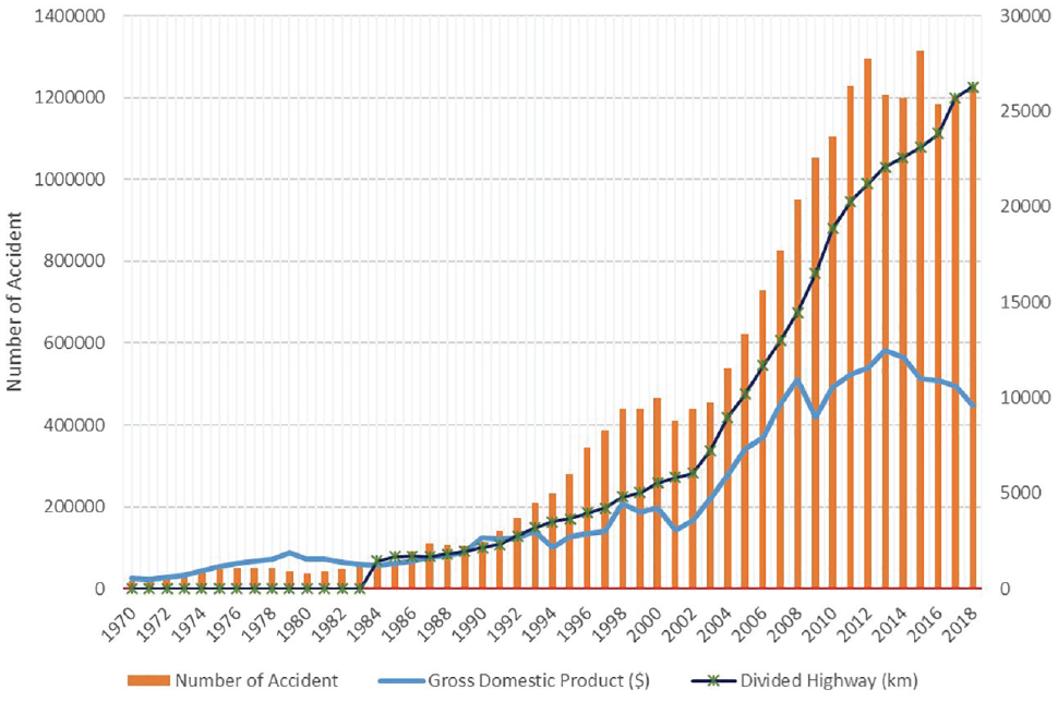
Number of accidents, gross national product (1970–2018), and divided road length (1983–2018).
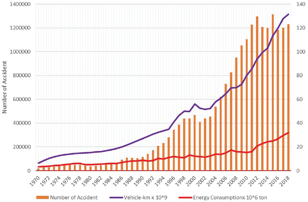
Number of accidents, vehicle kilometers traveled, and energy consumption (1970–2018).
Descriptive statistics of seven variables with logarithmic transformations are given in Table 1. Logarithmic transformation makes the data easier to interpret and creates a stable variance ( 32 ). Based on the descriptive statistics of the log transformed variables given in Table 1, the Jarque-Bera test shows that the variables have a normal distribution.
Descriptive Statistics
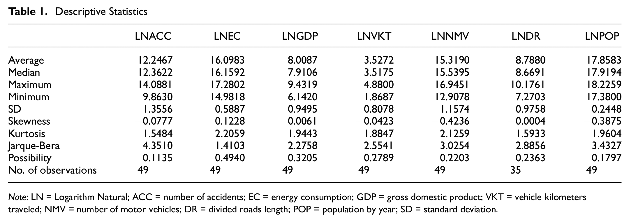
Note: LN = Logarithm Natural; ACC = number of accidents; EC = energy consumption; GDP = gross domestic product; VKT = vehicle kilometers traveled; NMV = number of motor vehicles; DR = divided roads length; POP = population by year; SD = standard deviation.
Methodology
The main aim of the study was to take the incidence of road traffic accidents in Turkey, examine the dynamic relationship between socioeconomic data, and investigate the causality of variables. For this purpose, the ARDL boundary test approach ( 33 ) was used to estimate the long-term equilibrium relationship between the six independent variables and the frequency of accidents. In this method, the existence of cointegration between time-series variables was examined and long-term relationships estimated. In addition, the short-term relationship was determined by the vector error correction model (VECM) approach ( 34 ). Unlike ARDL, which is designed to test cointegration, VECM assumes unknown structural relationships between variables ( 35 ). T-statistics and Wald tests can be applied to investigate the causality in the relationships examined with VECM. This approach is often referred to as “Granger causality testing within the VECM framework” ( 36 ). The ARDL and VECM approaches have been widely used in various countries and regions to detect the relationships between environmental factors such as CO2 emissions and economic variables such as GDP and energy consumption ( 37 – 39 ). However, few studies have examined the dynamic relationships between the frequency of traffic accidents.
ARDL Bounds Testing
In most time-series analysis studies, it is assumed that time series are stable or at least stationary around a deterministic trend. Thus, the internal dynamic properties of the series are ignored. Recent developments in this area have revealed that the series is not static in most cases. Therefore, some time series may move away from their averages over time, while others may approach their averages over the same period. In such a case, traditional methods may be misleading or inaccurate in determining the relationship between different time series. The researchers examined the existence of cointegration to overcome the problem of unstable time series. Cointegration can detect the presence of steady-state balance between variables using non-stationary time-series data ( 40 ).
ARDL is used to find the relationship between different time series by confirming the existence of cointegration. An ARDL model is used to explore a long-term equilibrium relationship by using the lagged and concurrent values of the independent variables together with the delays of the dependent variable ( 41 ). This approach is more advantageous than other cointegration methods ( 42 – 44 ).
The ARDL limit test model specified in this study is explained as follows:
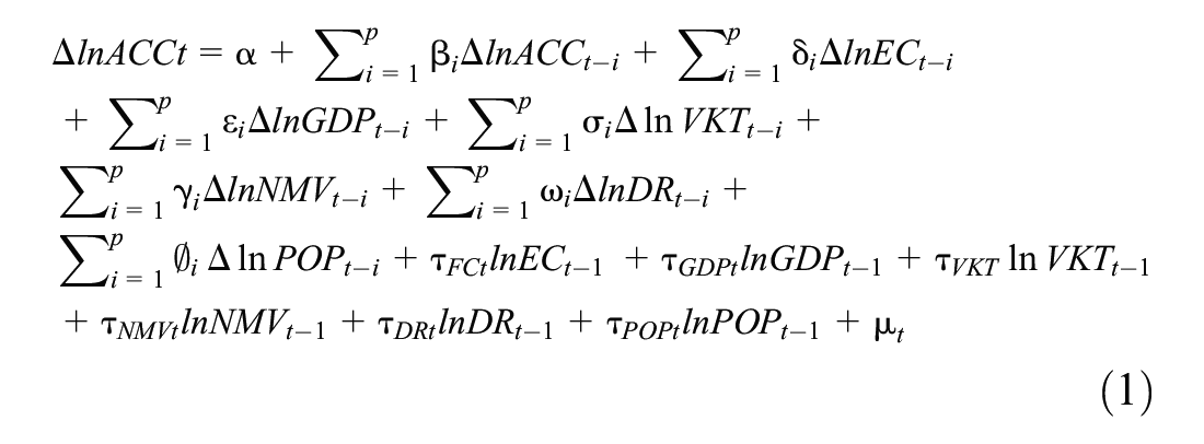
Here, ACC, EC, GDP, VKT, NMV, DR, and POP are shown. All variables are converted to their natural logarithm (LN) for better interpretation of the results. Δ Denotes the difference operator, α is a constant, μt is the error term, p is the maximum lag length and τEC, τGDP,τVKT, τNMV, τDR, τPOP respectively denote the long-term relationship for each variable. The terms with the additional signs belong to error correction dynamics.
In this study, the null hypothesis H0 is that there is no cointegration.

Rejecting the null hypothesis indicates the presence of cointegration. The null hypothesis is tested by the critical limits provided by the F-statistic and other studies ( 45 ). The following conditions hold:
If the value of the calculated test statistic is greater than the upper critical value, the basic hypothesis that there is no long-term relationship is rejected.
If the value of the calculated test statistic is less than the lower critical value, the basic hypothesis that there is no long-term relationship is accepted.
If the value of the calculated test statistic is between the lower and upper critical values, the stability properties of the variables should be found.
VECM Model
A vector autoregressive model (VAR) model is generally applied to determine short-term relationships between series. With this model, multivariate time series can be integrated by introducing the concept of error correction to represent short-term relationships between variables. However, there may be upward and downward movements in time-series variables by stochastic trends. In such cases, the VAR model can also be applied by re-parameterizing it as VECM. These features allow the VECM model to solve the so-called correlation problem in time-series analysis ( 46 ). VECM estimates a more efficient short-term coefficient than the limited representation of VAR ( 47 , 48 ). This approach has an advantage over traditional simultaneous equation models because the latter separates variables between two different groups (independent and dependent), while the former treats all variables on the same basis, that is, they are all assumed to be endogenous. However, a major disadvantage of this approach is that the same lag lengths must be assigned to relevant variables ( 49 ).
In our study, the VECM model is given as follows:
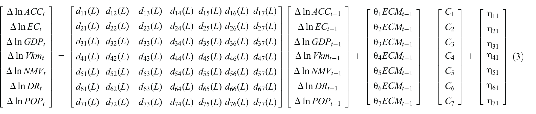
where
Ci; i ∈ {1,…, 7} are constants dij (L), and
i, j ∈ {1,…, 7} are polynomial functions of the delay operator L, ECMt−1 error correction term, θ coefficient of the error correction term and η error terms.
It should be noted that in the VECM framework, the coefficient of ECMt−1 is an important symbol representing the stability of the model, where a significant negative coefficient varying between 0 and 1 reveals a constant pattern of convergence toward equilibrium between multivariate time series ( 50 ). In our study, we performed a series of diagnostic and stability tests to ensure the fit of the model. These are serial correlation tests, normality tests, and different variance tests. To examine the stability, cumulative total (CUSUM), and cumulative sum of squares (CUSUMSQ) statistics are determined at the 5% significance level.
Granger Tests
The Granger ( 51 ) test, first proposed in 1969, is used to determine whether a series is useful in predicting others. Using previous values of a time series, the ability to predict future values can be measured. One of the advantages of VECM models is that they can test causation ( 52 ), by using the Granger procedure. When the Granger procedure is applied in VECM, it can capture both long and short-term causal relationships and reduce the risk of producing misleading results in the presence of counter action. Granger causality testing is performed by checking the significance of the coefficients by applying variable deletion tests obtained from the VECM model. Long-term causality is examined by t tests and short-term causality by F-statistics tests.
Results
ARDL Bounds Testing
The existence of the long-term relationship is checked by comparing the F-statistics with the critical limits of Pesaran et al. ( 45 ). Critical limits are valid only when the order of integration of any variable is less than or equal to 1. Therefore, a unit root test is applied as a first step to question the stationarity of each variable. For this purpose, the powered Dicky-Fuller (ADF) test, in which the variable has a unit root as a null hypothesis was applied. According to the statistical results shown in Table 2, according to the ADF unit root test, the series of variables LNACC, LNEC, LNGDP, LNVKT and LNPOP are stationary at 1% significance level in I (1). The series of the LNNMV and LNDR variables are stationary at 5% significance level, the first difference in I (1). The second difference of the LNEC variable in the series, I (1) is stationary at 1% significance level. This means that the null hypothesis containing the hypothesis that there is no unit root in level values is rejected.
Results of Unit Root Test
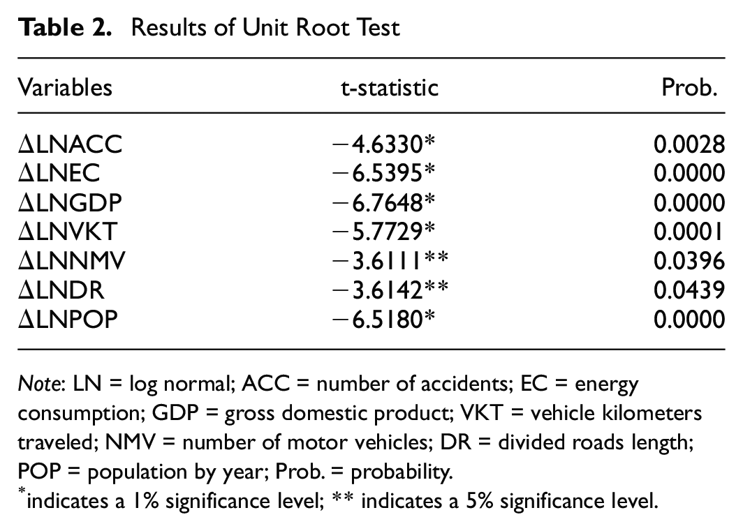
Note: LN = log normal; ACC = number of accidents; EC = energy consumption; GDP = gross domestic product; VKT = vehicle kilometers traveled; NMV = number of motor vehicles; DR = divided roads length; POP = population by year; Prob. = probability.
indicates a 1% significance level; ** indicates a 5% significance level.
Before proceeding to ARDL boundary tests, the Akaike information criterion (AIC) is used to choose the most appropriate lag length for each of the variables to balance the goodness of fit of the model with its complexity. It helps to better capture dynamic relationships between multiple variables. The results revealed that the optimum lag lengths for the examined variables are 1, 1, 0, 1, 0, 1, and 1.
The results of the ARDL limit test with the optimum lag length selected are presented in Table 3. According to Table 3, the H0 hypothesis is rejected because the F-statistic value (4.8589) calculated at the 1% significance level is greater than the upper limit (4.43) value. It has been determined that there is a cointegration relationship between the variables. After determining a long-term equilibrium relationship between variables with the F test, the estimation results obtained by the least squares method (LSM) of the variables reflecting this relationship are given in Table 4.
Results of Bounds Test
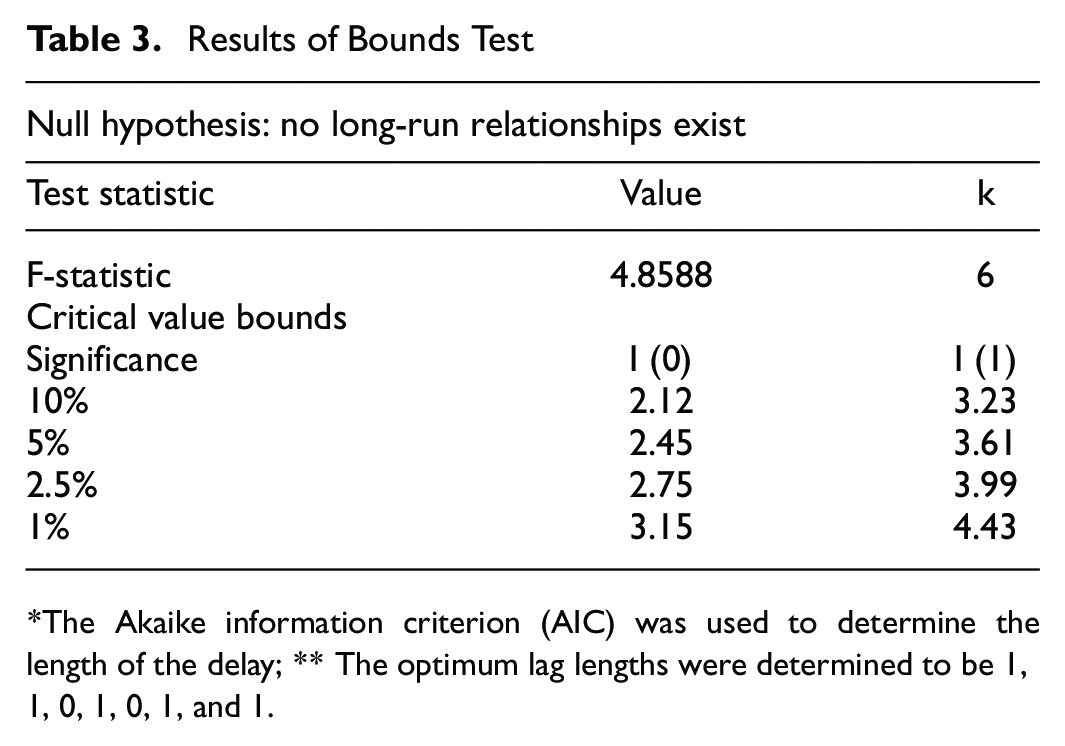
The Akaike information criterion (AIC) was used to determine the length of the delay; ** The optimum lag lengths were determined to be 1, 1, 0, 1, 0, 1, and 1.
Autoregressive Distributed Lag (ARDL) (1, 1, 0, 1, 0, 1, 1) Model Estimation Results
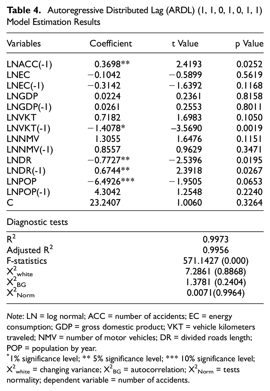
Note: LN = log normal; ACC = number of accidents; EC = energy consumption; GDP = gross domestic product; VKT = vehicle kilometers traveled; NMV = number of motor vehicles; DR = divided roads length; POP = population by year.
1% significance level; ** 5% significance level; *** 10% significance level; X2white = changing variance; X2BG = autocorrelation; X2Norm = tests normality; dependent variable = number of accidents.
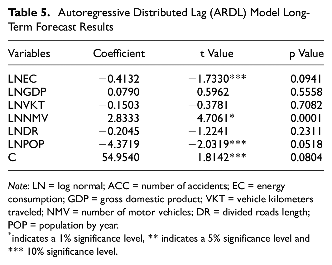
Since there was no problem with the variance (p = 0.8868), autocorrelation (p = 0.2404), or normality (p = 0.9964) in the model according to the diagnostic tests, an ARDL model was created to determine long-term relationships. Long-term estimation results calculated as a result of the ARDL model are given in Table 5.
Autoregressive Distributed Lag (ARDL) Model Long-Term Forecast Results
Note: LN = log normal; ACC = number of accidents; EC = energy consumption; GDP = gross domestic product; VKT = vehicle kilometers traveled; NMV = number of motor vehicles; DR = divided roads length; POP = population by year.
indicates a 1% significance level, ** indicates a 5% significance level and *** 10% significance level.
The variable of the number of motor vehicles has a statistically significant effect on the number of accidents at the 1% significance level. Energy consumption and annual population variables also have a statistically significant effect on the number of accidents at the 10% significance level. However, the variables of GDP, VKT, DR do not have a statistically significant effect. It is determined that a 1% increase in the number of motor vehicles increases the number of accidents by 2.83% according to a long-term perspective and it has a positive relationship with traffic accidents.
VECM: Short-Run Relationship
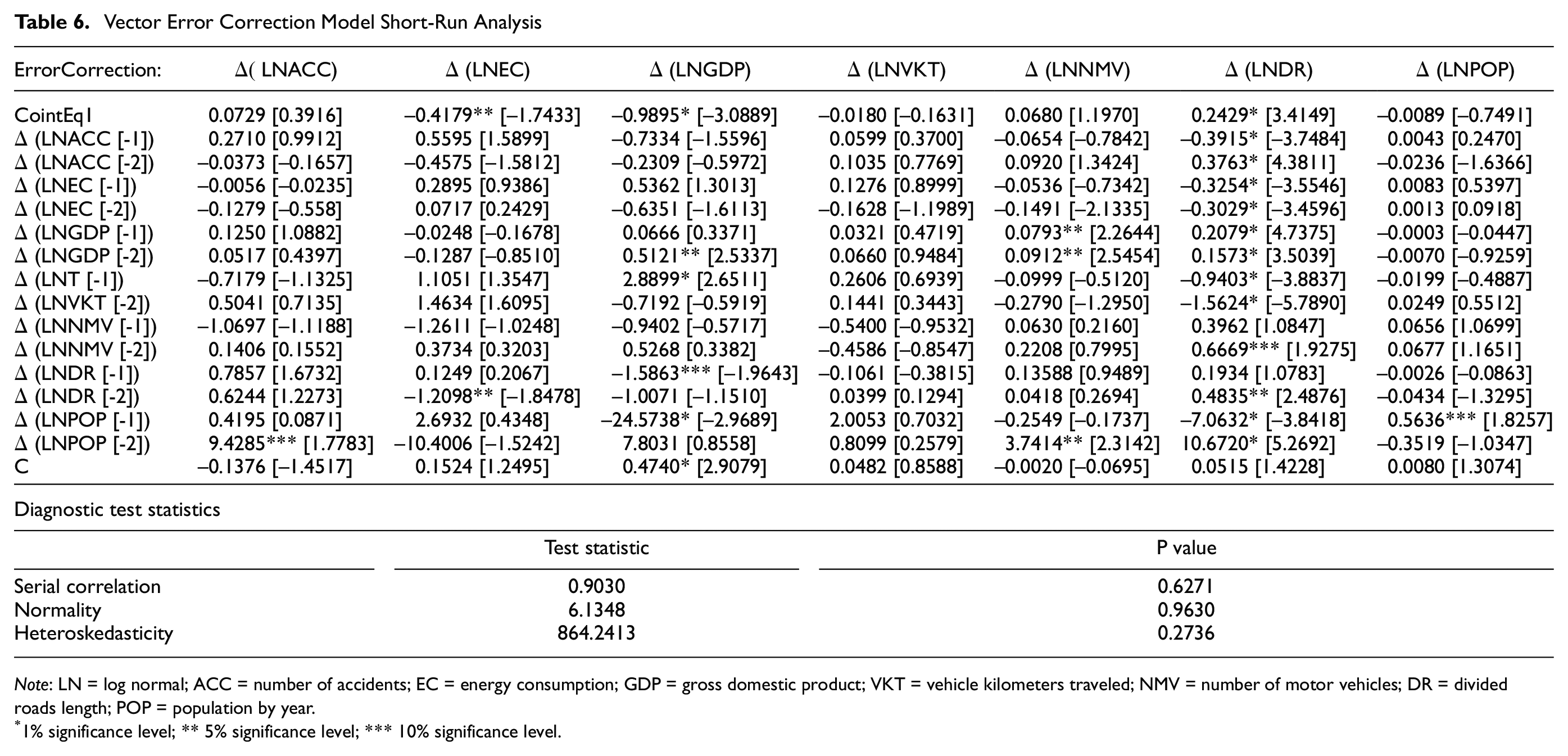
The results of short-term relationships within the variables using the VECM analysis are given in Table 6. The predictive coefficients of the error correction terms D (LNGDP) and D (LNEC) are −0.9895 and −0.4179, respectively, and they are both negative and significant at 99% and 95% confidence intervals. This finding confirms a robust and stable VECM model to examine short-term relationships when GDP and EC are considered as the dependent variables. In addition, the D (LNDR) error correction term estimation coefficient is 0.2429 and is positive and significant at the 99% confidence interval. There is a negative relationship found between DR and EC, in which the error correction term is found to be −0.3253 and significant at the 99% confidence interval: an increase in the DR decreases energy consumption. Diagnostic and stability tests are also applied to the model, and the results of diagnostic tests including serial correlation, normality, and heteroscedasticity, are reported in the lower part of Table 6. The results show that there is no serial correlation and no heteroscadasticity and the proposed model also passes the normality test. Cumulative sum (CUSUM) and cumulative sum of squares (CUSUMQ) graphs also verify the stability of the model. The cumulative total graph is given in Figure 4, and the cumulative sum of squares is given in Figure 5. If the CUSUM and CUSUMQ statistics are within the critical limits at the 5% significance level, it shows that all estimated coefficients in the VECM model are stable and reliable.
Vector Error Correction Model Short-Run Analysis
Note: LN = log normal; ACC = number of accidents; EC = energy consumption; GDP = gross domestic product; VKT = vehicle kilometers traveled; NMV = number of motor vehicles; DR = divided roads length; POP = population by year.
1% significance level; ** 5% significance level; *** 10% significance level.
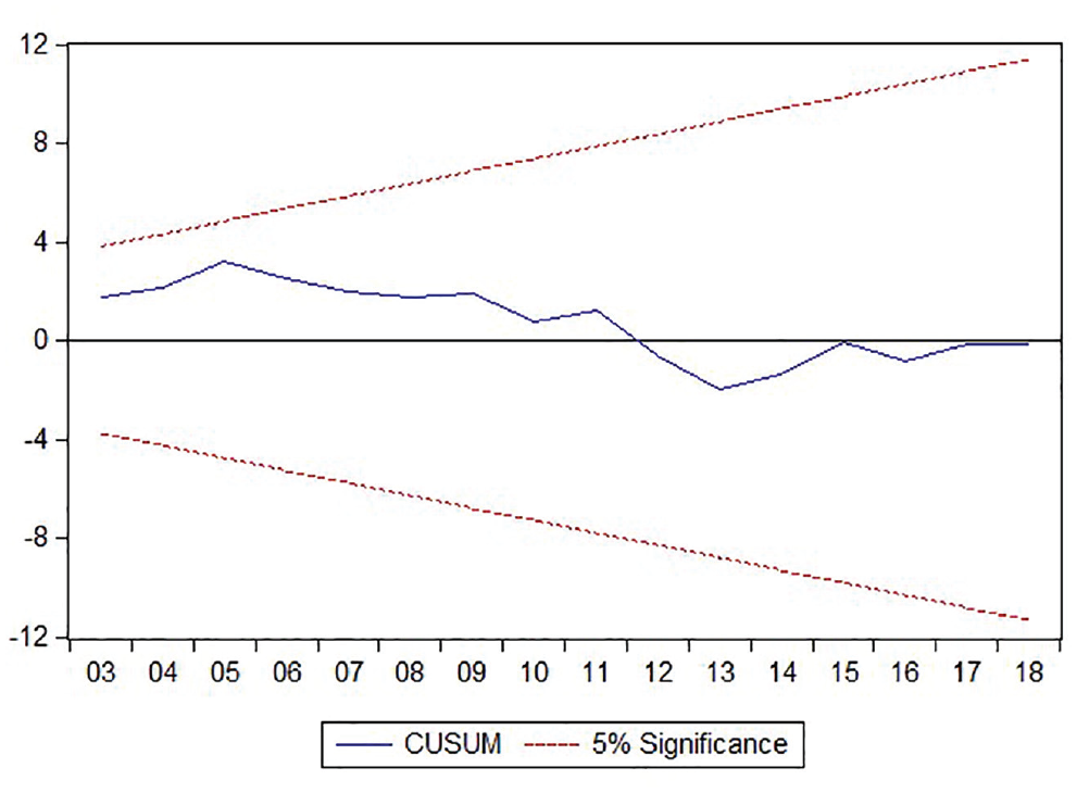
Cumulative total (CUSUM) test of recursive residuals dashed red lines show critical bounds at the 5% significance level.
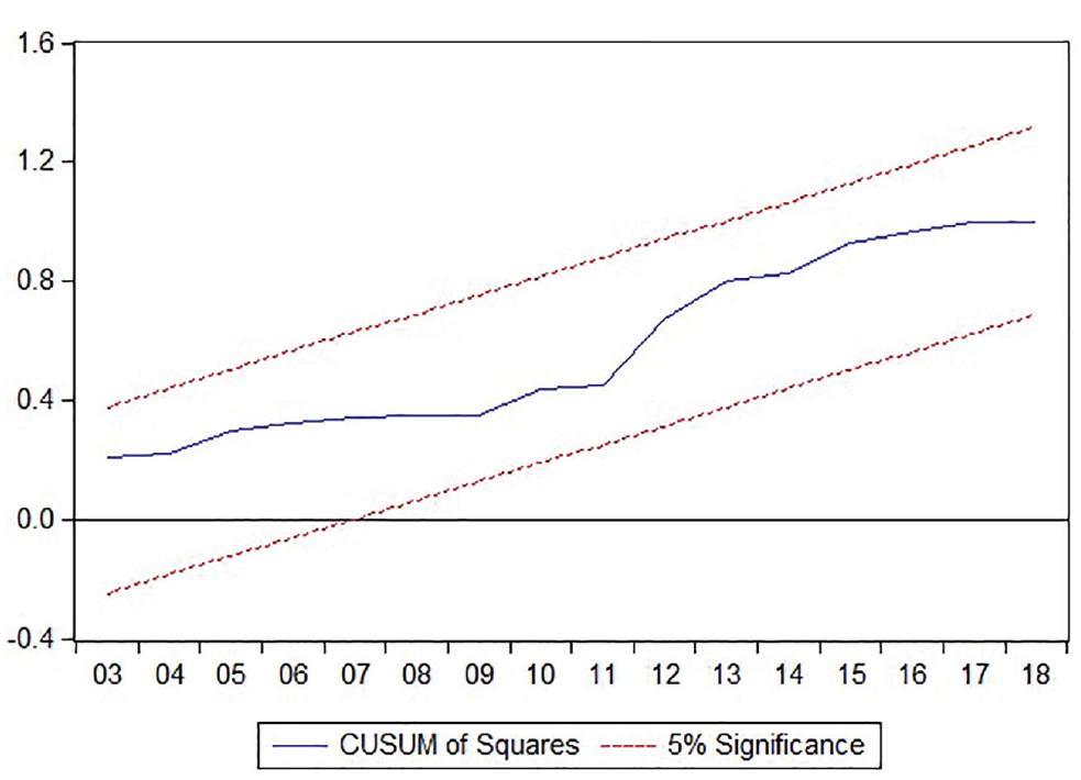
Cumulative total (CUSUM) squares test of the recursive residuals dashed red lines show critical bounds at the 5% significance level.
When the results of VECM short-term analysis are examined in Table 6,
Since there was no problem of variance (p = 0.2736), autocorrelation (p = 0.6271), or normality (p = 0.9630) in the model according to the diagnostic tests, the VECM model was created to determine short-term relationships. When the graphs in Figures 4 and 5 were examined, it was found that the short-term coefficients calculated in the VECM model had no structural breaks related to the variables and were stable, so the model could be estimated without using any artificial variables to express the breakage.
Granger Causality Analysis
Short- and long-term causality is tested by a Granger test in this section and the results are given in Table 7. When the Granger causality analysis results for the short-term VECM are examined, energy consumption is the reason for GDP; that is, the H0 hypothesis “not a cause” is rejected (p = 0,0366). VKT at the 5% significance level, DR at the 10% significance level, and POP at the 1% significance level are the reasons for GDP. At the 5% significance level, GDP and POP are the reasons for the NMV. At the 1% significance level, POP, VKT, GDP, EC, ACC, and NMV at the 10% significance level are the reasons for the DR.
Results of Vector Error Correction Model Granger Short-Run Causality
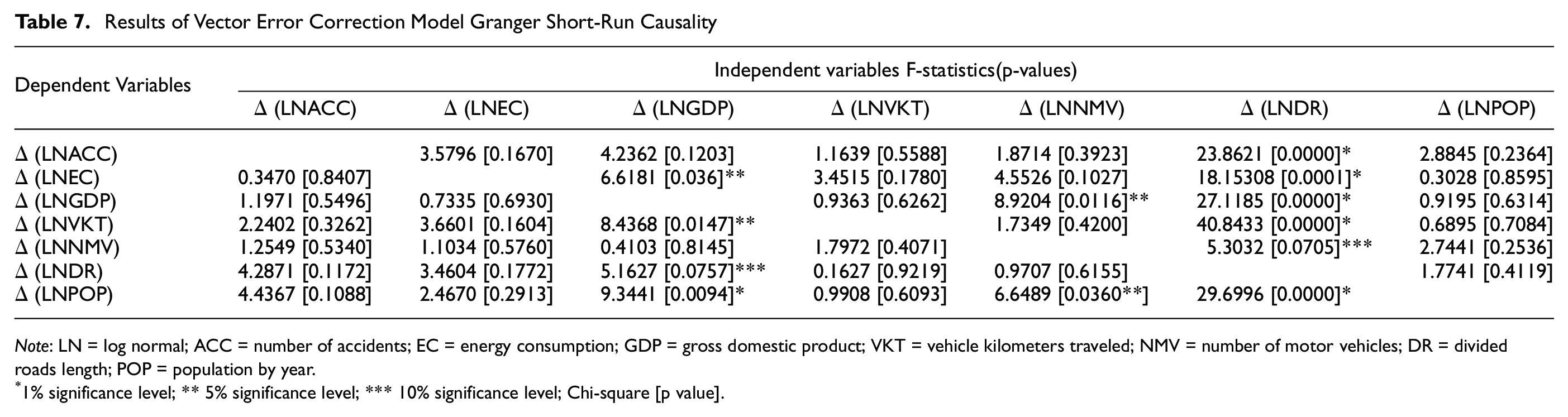
Note: LN = log normal; ACC = number of accidents; EC = energy consumption; GDP = gross domestic product; VKT = vehicle kilometers traveled; NMV = number of motor vehicles; DR = divided roads length; POP = population by year.
1% significance level; ** 5% significance level; *** 10% significance level; Chi-square [p value].
Conclusions
This article fulfills an important need in the literature by capturing dynamic relationships between selected socioeconomic variables and the frequency of traffic accidents in Turkey. During the 1970 to 2018 period, the contribution of the increase in energy consumption (EC), per capita GDP, vehicle kilometers traveled (VKT), the number of motor vehicles (NMV), divided road length (DR), and population (POP) to the number of traffic accidents (ACC) was examined. Eviews 10 program was used to analyze the data. The ADF unit root test was used to test the stationarity of the data. The ARDL boundary test approach was used to verify whether there was a long-term relationship between the time series of traffic accident data and socioeconomic variables. In addition, the VECM model was used to test whether there was a short-term relationship, and the Granger causality test was used to statistically evaluate the causality aspect of the relationship between variables. The analyzed socioeconomic variables, both the ARDL and the VECM results, statistically confirm the long-term relationship between EC, GDP, VKT, the increase in the NMV, DR, and ACC frequency with POP.
According to the long-term estimation results of the ARDL model, the variable of the number of motor vehicles has a statistically significant effect on the number of accidents at the 1% significance level. Energy consumption and annual population number variables have a statistically significant effect on the number of accidents at the 10% significance level.
However, the variables of GDP, VKT, and DR do not have statistically significant effects. The analysis determined that a 1% increase in the number of motor vehicles increases the number of accidents by 2.83% based on a long-term perspective and that it has a positive relationship with traffic accidents.
When the VECM short-term analysis results are examined, when
When the Granger causality analysis results are examined for the short-term VECM, energy consumption is the reason for GDP; that is, the H0 hypothesis “not a cause” is rejected (p = 0.0366). Similarly, VKT at the 5% significance level, DR at the 10% significance level and POP at the 1% significance level have a causative relationship with GDP. At the 5% significance level, GDP and POP have a causative relationship with the NMV.
At the 1% significance level, POP, VKT, GDP, EC, ACC, and NMV at the 10% significance level have causative relationships with the DR.
Footnotes
Author Contributions
The authors confirm contribution to the paper as follows: study conception and design: Salih BEKTAS; data collection: Salih BEKTAS; analysis and interpretation of results: Salih BEKTAS; draft manuscript preparation: Salih BEKTAS. All authors reviewed the results and approved the final version of the manuscript.
Declaration of Conflicting Interests
The author declared no potential conflicts of interest with respect to the research, authorship, and/or publication of this article.
Funding
The author received no financial support for the research, authorship, and/or publication of this article.
