



Abstract
Drones are increasingly being utilized to deliver medical supplies, and the COVID-19 pandemic has accelerated this trend. Drones arrive quickly by taking more direct paths and avoiding ground-based obstructions. However, drones are not completely reliable and may also experience failures and delays. For consumer products, delivery delays are an inconvenience, but for some medical supplies, delays may be fatal. This research focused on the drone reliability of one particular type of supply and event: automatic defibrillators for out-of-hospital cardiac arrests. A modeling framework was developed to analyze drone delivery reliability with stochastic demands and meteorological conditions. Using probability distributions based on real data from Portland, OR, this research quantified the failure rates as a function of drone range and meteorological conditions that included temperature, precipitation, and wind. Tradeoffs among drone reliability, fleet size, population size, and meteorological conditions were analyzed.
Drone deliveries are being tested across the globe to meet not only parcel delivery demands but also to open new service models and opportunities where traditional ground delivery methods are relatively slow and unreliable. The delivery of medical supplies is an area that has sparked high interest because such supplies are often subject to strict temporal constraints. For example, drones have already been employed for the delivery of medical supplies in Rwanda, a country that experiences heavy rains that often lead to road impassibility ( 1 ). Hospital supply chains in Rwanda now utilize drones for the delivery of blood from central storage facilities ( 2 , 3 ). Although blood deliveries are time-sensitive, some medical supplies are subject to even more stringent time considerations.
COVID-19 and the consequent lockdown have temporality removed some regulatory barriers for the deployment of drones. Drones are now being tested in several states such as Florida, North Carolina, North Dakota, and Virginia to deliver prescriptions, and there is a promising trial underway in Baltimore delivering kidneys for transplants ( 4 ). Even though there is the potential for a wide range of drone applications in the health sector, this research and case study focused on time-sensitive cardiac arrests.
Cardiac defibrillation ( 5 ) needs to be administered minutes after diagnosis to avoid patient death, but the majority (63%) of cardiac arrest cases occur outside of hospitals where defibrillators are not readily available. The survival rate for out-of-hospital cardiac arrest (OHCA) in 2016 was 12%, almost half that of the in-hospital rate (25%) ( 6 ). Currently, automatic external defibrillators (AED) weigh 1.1 kg (2.4 lb), take just 1.77 L (108 in. 3 ) of space, and come with instructions to guide nonmedical persons through the machine’s use ( 7 ). This makes AEDs an ideal candidate for drone delivery. However, the seriousness of cardiac arrest puts tight constraints on adequate arrival times. Even in hospitals, defibrillation survival rates after 3 min are reduced from 39% to 22%, and each additional minute reduces the chance of survival by approximately 4% ( 8 ). Currently, the average ground-based (ambulance) emergency response time in the United States is much longer than 3 min, with a mean of 7.0, 7.7, and 14.5 min for urban, suburban, and rural areas, respectively ( 9 ). As drones are not subject to typical ground road infrastructure restrictions, they may have a higher probability of timely response.
Pilots for medical supply deliveries using drones have begun in the United States ( 10 ), and recent research into drone deliveries of AEDs has attempted to quantify delivery times, estimate mortality rates, and optimize delivery networks through theoretical models ( 11 – 13 ). These studies have provided useful tools for AED delivery but have ignored key factors such as weather. Such exclusions and the lack of real-world data mean the viability of drone deliveries for time-sensitive supplies remains an open question.
This research focused on drone deliveries of AEDs for OHCA and fills a gap in recent research by using real-world data to model and assess the impact of weather on drone delivery reliability and to quantify the impact of fleet size and population on failure rates. Determining the number of drones required to service an area is challenging as the rate of cardiac events for an area is dependent on population size and time of day ( 5 ).
The remainder of this paper is structured as follows: first, demand and estimate failure rates are modelled as a function of drone fleet size and population for two types of drone operations: battery recharging and battery swapping. Second, temperature, precipitation, and wind using historical data from Portland, OR are modelled. Third, the impact of temperature, precipitation, and wind on range and drone delivery failure are quantified. Finally, conclusions, based on the results, are discussed with recommendations for future studies.
Modeling Demand, Fleet Size, and Failure Rate
The American Heart Association (AHA) provides a population mean

Modeling the number of occurrences in a given time interval is a common application of the Poisson distribution with parameter

Solving for

For any population,

Given this formulation, random OHCA events were simulated using a Poisson distribution with rate parameter
There was no statistically significant variation across months or seasons, but day-of-the-week and time-of-day did have significant variation. Incidence rate ratios (IRRs) with 95% CIs were used for simulation, where the highest increases were seen on Mondays (1.18, 1.38) and during the 8:00 to 9:00 a.m. hour (1.96, 2.59) (
15
). Combined, Monday mornings had an average rate increase of 2.91 over the yearly average OHCA rate. Normal distributions were assumed for each IRR, based on the central limit theorem of probability (
14
), and the time between consecutive OHCA events were simulated utilizing a Poisson process of rate
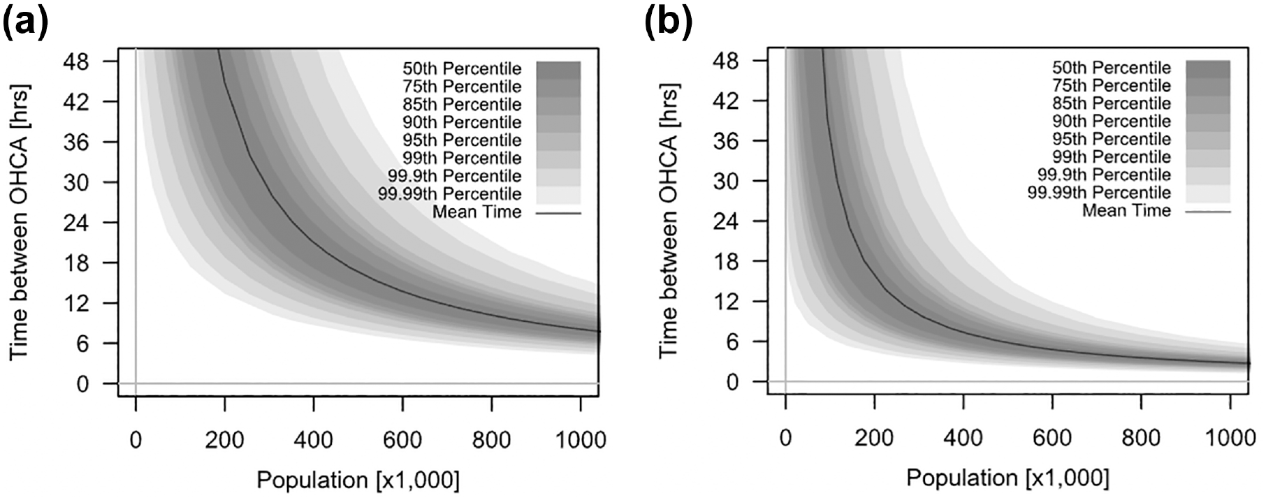
Time between consecutive out-of-hospital cardiac arrest (OHCA) events versus population for (a) U.S. average demand rate and (b) rate on Monday between 8:00 and 9:00 a.m.
Fleet Size, Drone Repositioning, and Battery Swapping Times
The number of required drones was based on the shortest time between events, given the nearly three-times increase over the average rates for Monday mornings, but also on the time it takes to serve a patient and reposition a drone. The calculated number of drones, therefore, was the minimum required during peak demand and above the minimum for all other days of the week and times of day. Two options were considered: in-drone battery recharging and battery swapping. For this study, we assumed that a high-performance multicopter MD4-3000 drone was utilized. Drone specifications are given in Table 1 ( 16 ).
MD4-3000 Drone Characteristics

Note: * wh = watt-hour, from source (17)
The optimal range was assumed to be 50 km (31 mi), which assumes ideal weather conditions and a cruise speed of 20 m/s (44.7 mph). With a 1.1 kg (2.4 lb) payload, the flight time will be approximately 42 min. The battery capacity of drones used in this study had a 21,000 mAh ( 17 ). The LiPo battery has a recommended recharge rate of 2A at greater than 90% charge efficiency ( 18 ). Therefore, the charge time following a complete drain of the battery for one of these drones is between 10 h 30 min and 11 h 40 min. However, batteries will not experience a full drain each time they are used, and there will be additional variability in the charge times based on distance traveled.
Given the random distribution of OHCA events and the combination of service and charge time of batteries, M/M/c queuing theory can be employed to determine the number of drones required. For service times, it was assumed that a drone must stay with a patient until the paramedics arrive (an average of 8 min) ( 9 ), stabilize the patient (averaging 2 min), have the automatic defibrillator repackaged for the return trip (averaging 5 min), and return to base (averaging 5 min of flight and landing time). In addition to these 20 min of service time, drones are additionally unavailable to service new patients while their batteries are being recharged (Case 1) or swapped for a fully charged battery (Case 2).
In Case 1, given an average of 10 min active flight time to and from a patient and an available flight time of 42 min, the average recharge time would be about 2 h 40 min. Adding the 20 min of service time, the average usage time was 3 h, which corresponds to an average of eight possible services per day. Using an M/M/c queuing model, failure was defined as the probability that there would be one or more people in the queue (i.e., a person is waiting to be served owing to drone unavailability). The rate of OHCA
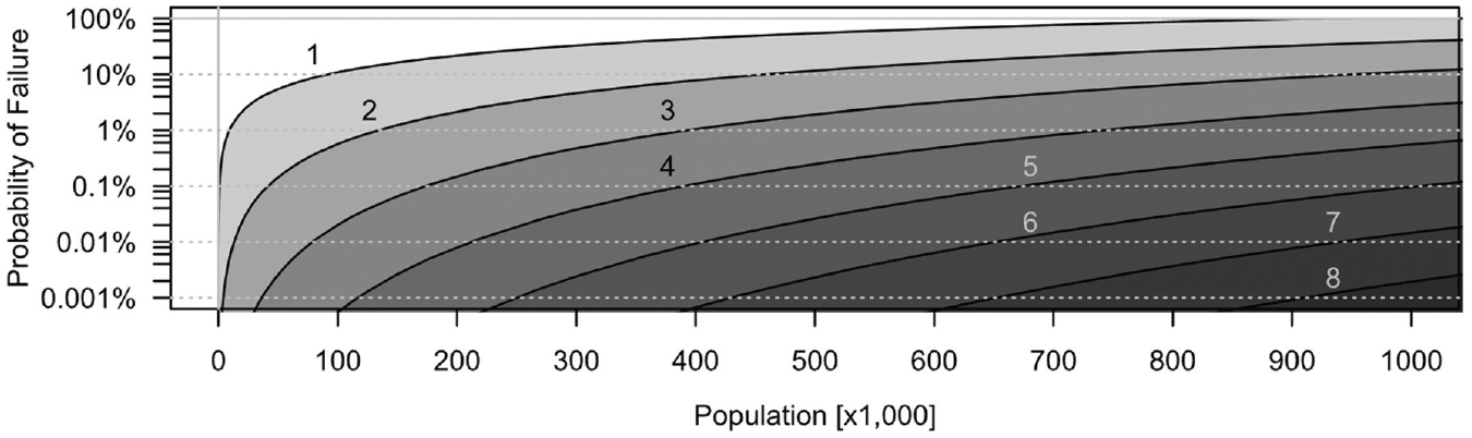
Case 1 (battery recharging): probability of failure versus population and number of drones given the demand rate on Mondays between 8:00 and 9:00 a.m.
In Case 2, after 20 min of average service time, each drone was assumed to be unavailable for an additional 10 min (30 min total) to allow for the battery to be swapped with a fully charged battery. Figure 3 gives the failure probabilities for Case 2 given M/M/c queuing theory using the Monday morning rate. By swapping batteries, the number of possible services per day increased by a factor of 6, from 8 (in Case 1, battery recharging) to 48 (in Case 2, battery swapping).
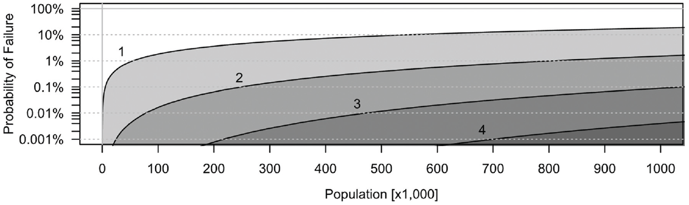
Case 2 (battery swapping): probability of failure versus population and number of drones given the demand rate on Mondays between 8:00 and 9:00 a.m.
For 100,000 people on Monday mornings, a single drone would fail to provide service 10.9% of the time in Case 1 versus just 1.8% of the time in Case 2. Picking an acceptable failure rate for vital medical supplies of <0.1%, three drones would be required in Case 1, and two drones in Case 2. For 300,000 people and a <0.01% failure rate, it would be five and three drones for Cases 1 and 2, respectively. This difference corresponds to notable cost savings; each drone can cost between $50,000 and $100,000 ( 19 ), but batteries cost between $300 and 600 ( 18 ). For 300,000 people and a failure rate of <0.01%, consider a theoretical requirement of one extra drone in both cases, and one or 10 spare batteries per drone in Cases 1 and 2, respectively. Equipment costs would be 30% less in Case 2. Lastly, other extreme conditions, such as those caused by wildfires, are potential issues, but were outside the scope of the paper given the lack of detailed long-term wildfire data, the unique complexity of this topic, and the unusual set of operating constraints. A further potential issue is maintenance time and the mechanical reliability of drones, but this topic was also outside of the scope of this paper owing to the lack of drone reliability data.
Weather Modeling
Modeling Temperature Data and Distributions
Historical temperature data for a region typically gives a mean, high, and low temperature for each daily record. Figure 4 shows a histogram of January and July daily high temperatures from historical tables from Portland, OR. Given the shape of the temperature histograms, each month’s high and low temperatures were assumed to follow a normal distribution. Therefore, historical data provide the ability to calculate means for high and low temperatures and their respective standard deviations for simulation. However, on a given day, high and low temperatures are highly correlated, and this must be considered for simulations.
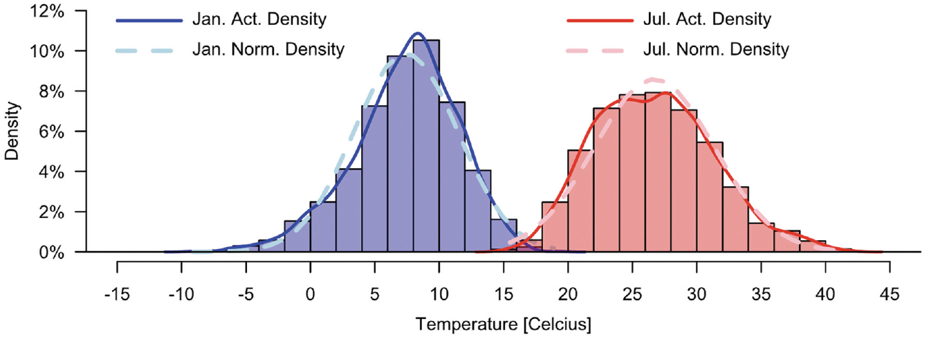
Histogram, density, and normal approximation of historical high temperatures for January and July.
To generate a pair of correlated random normal variables,

where

Using
Historical Monthly High and Low Temperatures (°C) and Correlation Factors
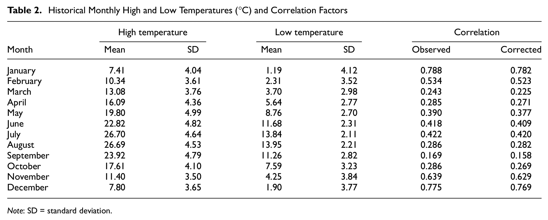
Note: SD = standard deviation.

The probability that the average daily and 8:00 a.m. temperatures are less than 0°C is important to the calculations of precipitation; as such, the increases are also important for future predictions. For any normally distributed variable,

In addition, the sum of any two normally distributed variables,

For average daily temperature, the distribution of average temperature can be found by averaging the distributions of high and low temperatures. Given means,

The probability that the average daily temperature is less than 0°C can be directly calculated for this normal distribution. This section presents the general statistical framework to analyze temperature. In the specific application and case study, at 8:00 a.m. (worst-case scenario), the probability was based only on the distribution of low temperatures.
Modeling Precipitation (Rain and Snow) Data and Distributions
Many regions have systems to measure rainfall. Often, the amount of rain per day and the amount of snow per day are included. For precipitation generally in the United States, 13 in. (33 cm) of snow equals 1 in. (2.54 cm) of precipitation. This conversion allows for total precipitation per day to be calculated. The same weather data set for Portland, OR, provided historical rain and snow measurements, which were combined. Table 3 shows the estimates for the mean and variance of precipitation on days with rainfall, and the calculated percent of days without rainfall for each month.
Probability of Zero Rain on a Given Day, and Daily Means and Variances of Precipitation for Each Month

As with temperature, precipitation can be aggregated by month to account for monthly variation and subdivided into two distributions: Bernoulli probability of precipitation versus no precipitation, and a gamma distribution for the quantity of rain, given some rainfall (
23
). Given the daily average,

A scalar constant applied to a gamma distribution is still gamma (
24
). For an hourly distribution,
For example, there was a 9.2% probability that the average daily temperature in January 2020 would be less than 0°C and a 32.6% probability of no rain. As such, the probability of snow was 6.2%, which corresponds to an average of 1.9 snowy days in January. However, during 8:00 a.m., there was a 30.5% probability temperatures would be below 0°C in 2020. Given the same probability of some rain, there was a 20.6% probability of snow during that hour, which corresponds to 6.4 mornings with some snow.
Modeling Wind Data and Distributions
A key factor that influences aviation performance is wind, and drones are highly susceptible because of their limited power and weight. The distribution of wind speeds can be modeled using a variety of known probability distributions with the Weibull ranking being among the best ( 25 ); however, several models have been shown to be adequate. The creation of wind models is dependent on both the amount of historical data and the temporal granularity. For example, the inclusion of only a daily mean will not be sufficient to define most parametric models. However, a generalized understanding of wind effects does not require the accuracy of several climate models. As such, the choice of a probability distribution should be based on what can provide a reasonable approximation based on the available data ( 26 ).
There are long time series for Portland wind data, including historical average speeds, maximum gusts, percent calm, and direction. Gradient descent optimization was employed to find distribution parameters that provided reasonable approximations of historical trends. In Portland, different times of the year have different distributions of wind, which will directly influence failure odds. The distribution of wind speeds over a year is given in Figure 5.
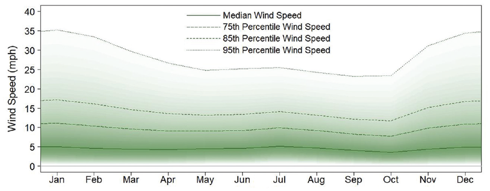
Simulated mean and confidence interval of wind speed in Portland, OR.
Wind direction is also important. In Portland, winds mostly blow in the east-southeast direction during the winter months and the northwest direction during the summer months (see Figure 6). This factor is important for determining a drone’s range at different times of the year. In January, areas to the northwest of a depot will be restricted by a headwind, whereas the opposite is true in July.
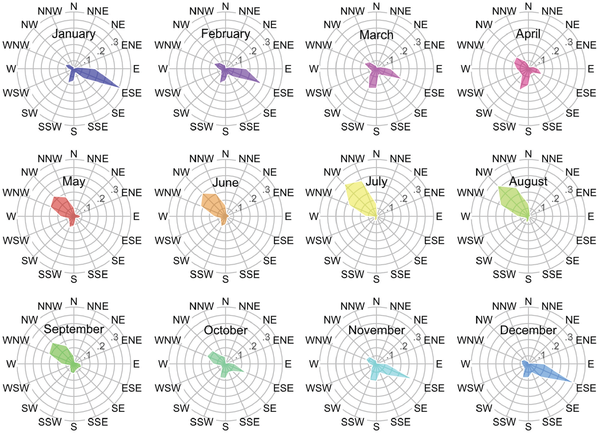
Probability of wind direction for each month in Portland, OR.
Range Reliability Modeling
The range of a drone is determined by its weight, flying efficiency, and battery capacity. For applications with a central hub, this range is half the distance a drone can travel, as a return trip must be accommodated. The following gives the energy necessary for level flight ( 16 ):

where
From Equation 1 it is possible to observe that energy consumption is directly proportional to drone mass and travel time and distance. The range estimations of this research considered the defibrillator 1.1 kg (2.4 lb) payload.
Modeling the Impact of Temperature
Temperature can have a significant impact on drone performance because drone lithium-ion batteries show optimal performance at approximately 20°C (68°F) but perform significantly worse at lower temperatures (see Figure 7). For lithium batteries, the output voltage is dependent on its operating temperature ( 27 ). In this study, battery available energy or capacity was assumed to decrease following a parabolic curve. The maximum (100%) will be at 20°C (68°F) and the minimum (50%) at −20°C (−4°F). At higher temperatures, the capacity decreases linearly from 100% to 95% from 20°C (68°F) to 55°C (131°F). Battery makers recommend no operation outside this temperature range ( 18 ).
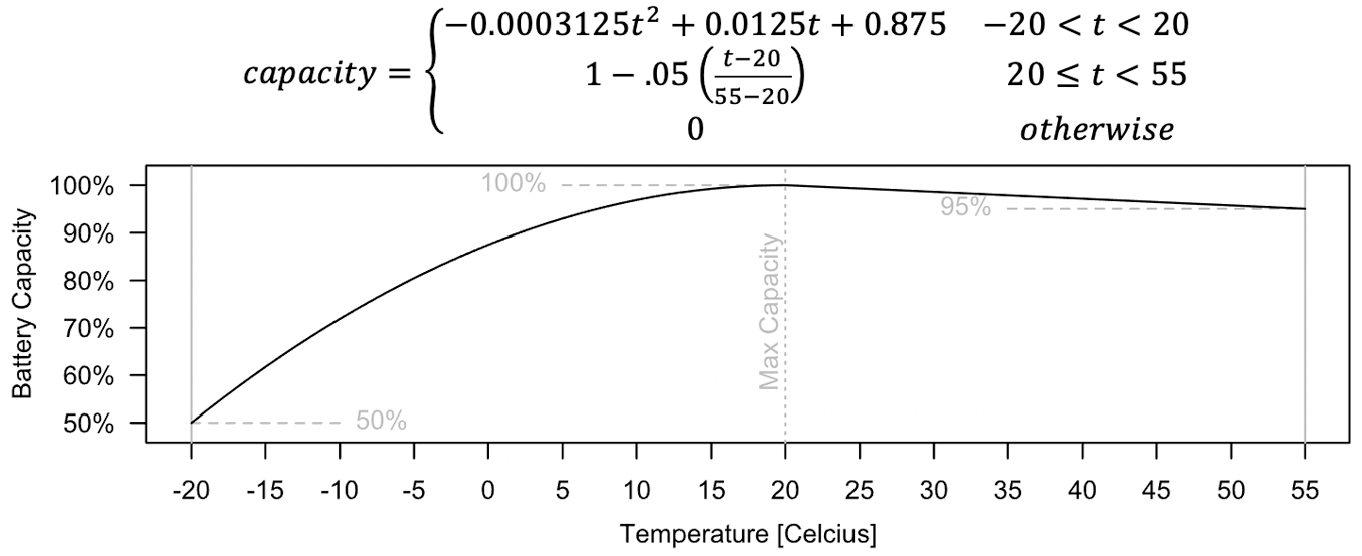
Battery capacity versus temperature and equations.
In addition, battery capacity degrades linearly with the number of cycles up to a point. Often, the degradation accelerates when a battery reaches 80% of optimal capacity. At this point, the battery is considered unreliable and is no longer used. Before this point, the battery will have above 80% optimal capacity, but the exact amount will be unknown for any specific trip. As such, a random uniform distribution from 0.8 to 1.0 can be used in association with temperature for simulation to define the initial condition of the battery with an assumption that faulty or unreliable batteries will not be used.
OHCA events are more frequent during the 8:00 a.m. hour, which is typically the coldest hour of the day. As such, only the distribution of low temperatures is needed in this study. Figure 8 shows the means and CIs for daily high and low temperatures.
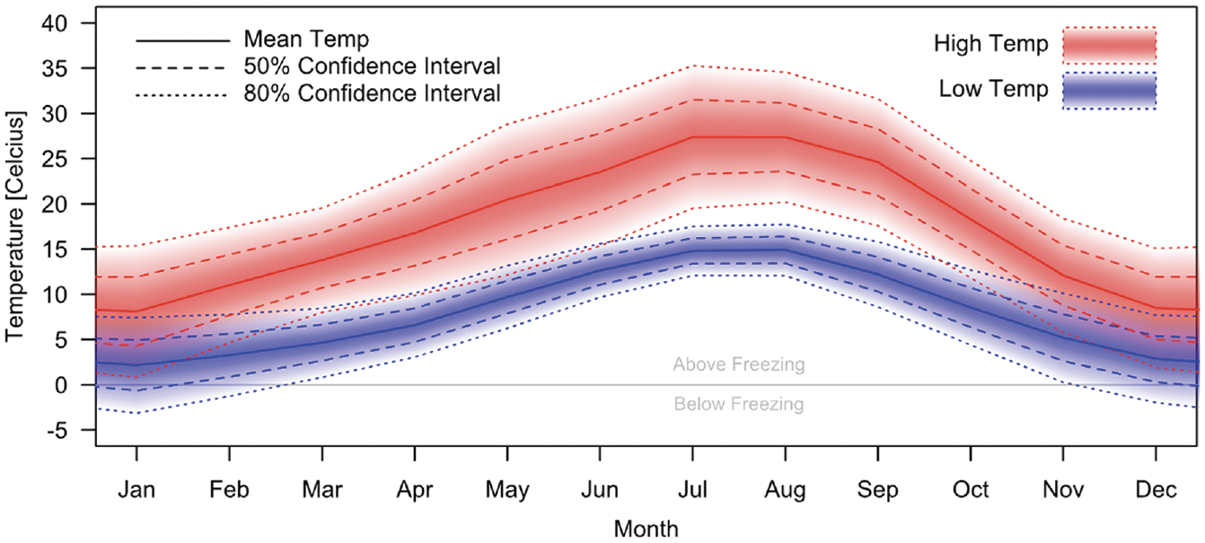
Means and confidence intervals for high and low temperatures by month.
Figure 9 shows the probability of failure as a function of the total distance traveled, assuming an ideal 42-min flight time. The left and right edges of the shaded regions are defined using distributions of the low and high temperatures, respectively. The purple area is based on the yearly average highs and lows, whereas the blue region represents the worst-case (i.e., coldest) temperatures in January. The potential range of a drone will be half the total available flight distance, as return trips must be accommodated. The probability of failure is the percent of simulated trips that failed to reach a given range.
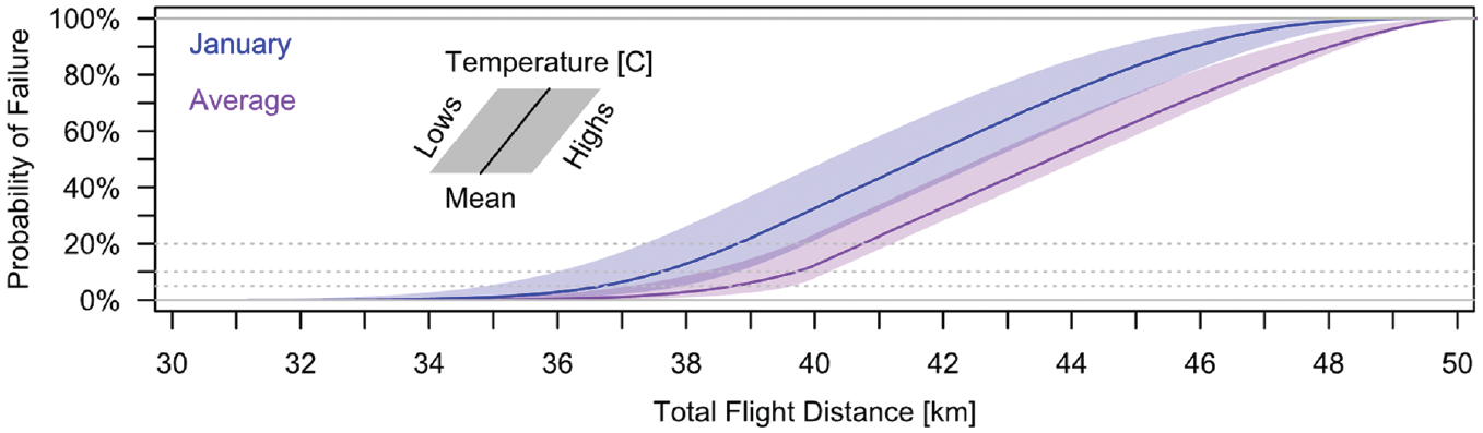
Probability of failure owing to temperature and available battery charge versus flight distance.
Winter will have the worst-case flight ranges as compared to the yearly averages. Yet, the range in the worst case was still larger than the maximum allowable in relation to time constraints for urgent medical deliveries. Even allowing for 14.5 min of flight time—the average ambulance arrival time in rural areas—more than 95% of drones would have enough charge for the 35-km (22-mi) trip, 17.5 km (11 mi) in each direction.
In addition, the available range corresponded to a large service area. The 3-min delivery area covered 40 km2 (15.7 mi2), whereas 7 min (the urban ambulance average response time) allowed for an area of 222 km2 (86 mi2). This is functionally the size of many cities. Based on Portland weather conditions, large cities would require just a few drone hubs for full coverage.
Modeling the Impact of Precipitation
Several modern drones advertise some resistance to rain. As such, not all precipitation events would be considered failures. Considering rain alone (i.e., no snow), defining a specific cutoff for the permitted amount of rain would result in different failure odds. Figure 10 shows probability failure (plotted logarithmically) as a function of the maximum allowable precipitation rate. As an example, if drones are not sent during heavy rain, then drones will be unavailable (a failure condition) 4% of the time in January and <0.1% of the time in July.

Probability of failure as a function of rainfall rate cutoff.
Most drone manufacturers recommend not flying drones during snowfalls. As such, all snowy weather would cause a failure condition. However, if the amount of snow is considered such that some snowfall is acceptable, the failure rates would also be dependent on the precipitation cutoff (see Figure 11).
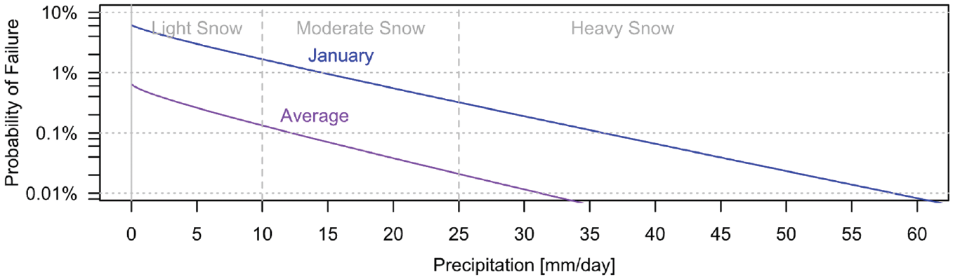
Probability of failure as a function of snowfall rate cutoff.
The cutoff points for snow and rain do not need to be equal. For example, if drones are permitted to fly in snow up to 10 mm/day (light snow) and rain up to 25 mm/day (light and moderate rain), then drones in January would be unavailable about 2% of the time because of snow and about 4% of the time owing to rain.
Modeling the Impact of Wind
For winds, the worst case is a headwind where the flight path is directly against the wind’s direction of travel. In the best case, the drone has an increased speed resulting from a tailwind. Given a wind bearing, its speed, and a drone’s flight speed, an angle-side-side triangle is formed (Figure 12). This arrangement requires an algorithm to solve as there might be 0, 1, or 2 possible answers. The following algorithm can be used to solve for the fastest feasible flight path, if possible. It combines the law of cosines and solves for the unknown using the quadratic formula.
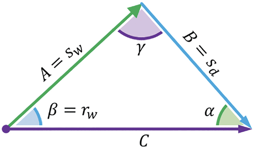
Setup and notation to solve an angle-side-side triangle, where
Beginning with the law of cosines, where side
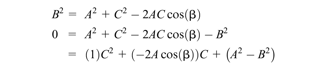
Solve for
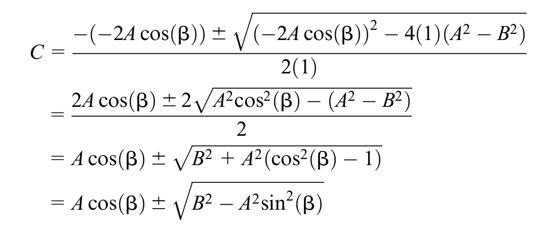
Mathematically, there are potentially two solutions,

However, in the context of flight speed triangles, negative and imaginary solutions are not applicable, and the fastest speed is preferred. Given that
As an example, assume a drone speed of 20 mps, wind speed of 30 mps, and a wind direction 30° away from the travel direction; both triangles in Figure 13 are valid solutions where the drone flies at a 20 mps and is able to reach the destination. The key factor is the effective travel speeds and initial flight bearings. A drone using the initial travel bearing from the second triangle would reach its destination three-times faster than a drone using the initial bearing from the first.

Two valid solutions to an angle-side-side triangle problem.
For headwind and tailwind simulations, flight times were held constant for arbitrarily selected 2-min and 10-min cases. For each trial, distance traveled within the time limit was recorded. The probability of delivery failures from wind was calculated based on the percent of trips that failed to reach a given distance within the allowable time. The shaded regions of Figures 14 and 15 show a range of failure probabilities between a simulated headwind versus a simulated tailwind and the result using a random bearing as the central line. As the flight time increased, the probability of failure also increased. In Figure 15, the y-axis of Figure 14 is transformed from linear to logarithmic.

Probability of failure versus radius from wind with linear y-axis.

Probability of failure versus radius from wind with logarithmic y-axis.
At a 20% acceptable failure rate for 2-min deliveries, the worst case for the range decreased from 2.4 km (1.5 mi) to about 2 km (1.2 mi)—a reduction of 16%. At a 5% acceptable failure rate, the range further reduced to about 1.3 km (0.8 mi). Although the theoretical range of drones is large (see Figure 9), the practical range for timely deliveries is a limiting factor.
Figure 15 shows that the average potential failure from wind is above 0.1% for a 2-min or 10-min trip. Wind plays a key role in determining acceptable failure rates and for determining a potential range for drone deliveries. Notably, having multiple hubs would reduce failure rates from the wind as different hubs could be employed depending on wind direction. Headwinds and potential failure from one direction could be tailwinds and success from another.
Conclusions
For the delivery of time-sensitive supplies, drones might provide the means to bypass many obstacles experienced by ground transportation. However, drones are subject to their own set of constraints that limit the likelihood of successful deliveries. Although packages from an online retailer can be delayed by hours without substantial ill effect, even short delays in the context of medical supplies can be fatal. This research utilized real-world data to examine the impact of stochastic demand and weather conditions on drone delivery reliability.
The number of drones needed is highly dependent on charge times, use of battery swapping, and population in the service area. The specific application of drones to deliver defibrillators must consider that the average OHCA demand rate increases 2.91 times on a Monday morning. This worst-case scenario and economic considerations should be used to define the required equipment for a service area. Additional consideration should also be given to potential mechanical failures and maintenance schedules. Given the equipment costs, one potential solution is a requirement for one extra drone over the calculated minimum, extra batteries, and equipment to check battery health. Lastly, it is important to note that failure because of extreme weather conditions cannot be addressed by simply having more available drones. Extreme weather conditions that would result in a failed delivery for one drone, would result in a failed delivery for any other drone because drones cannot operate under extreme weather conditions. In summary, proper fleet sizing could address variability in demand as well as variability in weather conditions but will not eliminate delivery failures resulting from extreme weather conditions when drones cannot operate.
In this case study, wind was a key factor; even the average winds of Portland in January would cause failures, defined by travel time constraints more than 1% of the time. The direction of winds also changes depending on the time of year. The placement of drone hubs should consider ranges defined both by temporal constraints given by OHCA events survival rates as well as probabilistic failure odds caused by winds. Studies that examine multiple hubs could also consider potential failure rates and repositioning strategies considering the seasonality of weather conditions.
The temperature in Portland was not as crucial as wind in relation to reliable drone deliveries. The large potential delivery range of high-quality drones combined with strict delivery time limits reduced the negative effects of temperature and charge cycles. Therefore, temperature, as it relates to battery function, could be ignored for these types of deliveries since the potential for failure remained low. For example, a 14 km (8.7 mi) trip (28 km or 17.4 mi both ways) would have less than 0.001% failure odds owing to temperature and charge decay in the worst case. Although extreme temperatures have limited negative effects on batteries, wildfires, a cause of such extreme conditions, could potentially limit drone operations owing to difficult operating conditions and “no-fly orders” issued by federal, state, and local wildland fire management agencies and the Federal Aviation Administration (FAA) ( 28 ). Wildfires are an important issue, but outside of the scope of this paper owing to the lack of detailed historical data required to model and predict wildfire intensity, winds, location, and so forth. These issues are compounded by a dynamic problem from greenhouse gas emissions and their effect on wildfire characteristics and seasonality.
Precipitation failures are highly dependent on the level of precipitation considered too high to send a drone. The rate of failure, defined by the probability of not sending a drone, changes throughout the year and by time of day. If a drone is rated for higher water resistance, the failure rate will be lower. Furthermore, temperature is important as it relates to precipitation, as snow has larger adverse effects on drone operations compared with rain.
This paper has examined several of the mechanical and meteorological impacts on drone deliveries to examine which factors are most important and to define limits. The results indicated that successful drone deliveries of AEDs were highly influenced by wind speeds, wind direction, and precipitation rates; however, ambient temperature may mostly be ignored for short and strict delivery time limits. Furthermore, battery swapping could be highly effective at reducing equipment requirements given worst-case demand.
Given adequate historical data about weather and demand, drone delivery operators should be able to plan efficiently to meet peak demand periods without unacceptable failure rates or excessive costs. Winds will remain an obstacle during some parts of the year unless drone speeds can be improved. Although drones could provide fast delivery times for the vast majority of cases, some failures would be difficult to avoid. Ideally, service areas should remain small enough that travel times are not limited by distance, and overlap of service hubs would provide alternative delivery routes when wind direction is not ideal.
Future research could also examine the likelihood that the delivery of automatic defibrillators would be operable, given that only one-third of OHCA are witnessed by another person. This paper assumed 100% reporting for OHCA events; as such, the rate,
Furthermore, there is an access and equity question associated with a drone’s ability to deliver to some areas. For example, airports are often restricted flight zones that do not allow drone operations. Such areas are also areas with higher proportions of lower-income communities. Future research could examine where a delivery system could be employed and what ground delivery systems would be required locally to adjust for access differences. In addition, future research efforts should analyze how COVID-19 and subsequent lockdowns have greatly increased opportunities to deploy fleets of drones for time-sensitive deliveries.
Footnotes
Author Contributions
The authors confirm contribution to the paper as follows: study conception and design: M. Figliozzi, T. Glick; data collection: T. Glick, M. Figliozzi; analysis and interpretation of results: T. Glick, M. Figliozzi, A. Unnikrishnan; draft manuscript preparation: T. Glick, M. Figliozzi, A. Unnikrishnan. All authors reviewed the results and approved the final version of the manuscript.
Declaration of Conflicting Interests
The authors declared no potential conflicts of interest with respect to the research, authorship, and/or publication of this article.
Funding
The authors disclosed receipt of the following financial support for the research, authorship, and/or publication of this article: This research was funded by the Freight Mobility Research Institute, a U.S. Department of Transportation University Transportation Center.

Opinions given as well as any errors or omissions are the sole responsibility of the authors.