
Abstract
The emergence of connected and autonomous vehicles (CAV) is of great significance to the development of transportation systems. This paper proposes a multiple-factors aware car-following (MACF) model for CAVs with the consideration of multiple factors including vehicle co-optimization velocity, velocity difference of multiple PVs, and space headway of multiple PVs. The Next Generation Simulation (NGSIM) dataset and the genetic algorithm are used to calibrate the parameters of the model. The stability of the MACF model is first theoretically proved and then empirically verified via numerical simulation experiments. In addition, the VISSIM software is partially redeveloped based on the MACF model to analyze mixed traffic flows consisting of human-driven vehicles and CAVs. Results show that the integration of CAVs based on the MACF model effectively improves the average velocity and throughput of the system.
Keywords
Connected and autonomous vehicles (CAV) are thought to be a vital component for future transportation systems because of the possibility of precise control of individual vehicles and the resultant positive effects such as smoothing traffic flow, increasing throughput, and improving traffic safety ( 1 – 7 ). However, the driving behaviors of CAVs are likely different from those of human-driven vehicles (HV) because of their autonomy and connectivity. For example, CAV platooning may lead to smaller headways between two consecutive CAVs compared with a pair of disconnected HVs. Further, the connectivity between vehicles (and maybe even between vehicles and infrastructure) makes it possible for a CAV to obtain information of surrounding vehicles within the communication range rather than just information of vehicles closely around. While not available in HV traffic, this information likely affects the driving behaviors of CAVs. To accurately control individual CAVs, and thus to realize the potential benefits of CAVs, fundamental efforts are needed to understand the driving behaviors of CAVs.
Car-following model is one of the traditional topics in urban transportation studies focusing on the longitudinal driving behaviors of vehicles. Given a stream of vehicles on a single-lane highway, car-following models describe how a following vehicle (FV) follows preceding vehicles (PV). In early studies on car-following behaviors of HVs, the FV’s motion is assumed to be determined by its own state and the state of the closest PV, such as the General Motors’ (GM) model, the optimal velocity (OV) model, the full velocity difference (FVD) model, the intelligent driver model (IDM), and Gipps’s model ( 8 – 12 ). With the emergence of CAVs, some scholars have proposed car-following models for connected vehicles based on traditional car-following models. Among them, probably the most well-known are the adaptive cruise control (ACC) model and the cooperative adaptive cruise control (CACC) model ( 13 , 14 ). These two models consider the acceleration and speed of only the closest PV. Besides, Hasebe et al. proposed an extended OV model that allows each vehicle to be affected by the information of an arbitrary number of PVs and FVs ( 15 ). Ge et al. considered backward-looking effects, and proved that the stability of traffic flow is affected by both forward-looking and backward-looking information ( 16 ). Yu et al. extended the FVD model by incorporating headway interaction, velocity difference, and acceleration of the PV ( 17 ). In addition to considering the optimized speed functions related to multiple PVs, these three models take into account other factors of the PVs (e.g., the distance between PVs, the speed difference, and the acceleration of PVs). Recently, some scholars have gradually started to show interests in car-following models for AVs. Gerardo et al. modeled the car-following behaviors of AVs by considering the information of one PV ( 18 ). Wen-Xing et al. proposed a new car-following model for AV flow using the mean expected velocity field ( 19 ). Fu et al. proposed a human-like car-following model for autonomous vehicles (AVs) by considering the cut-in behavior of other vehicles in mixed traffic ( 20 ). These three models are mainly based on the characteristics of AVs, and other factors, such as cut-in behavior and mean expected velocity field, are also taken into account.
However, most of previous research on car-following models are based on classic models and thus typically consider only a few factors. For example, the traditional OV model assumes that the driving behavior of the FV is only affected by the closest PV. In fact, the driving behavior of the FV will also be affected by other factors, such as the velocity difference and space headway of other PVs. These factors have not been considered in car-following models for HVs because of HVs’ inability to exchange information. However, multi-vehicle information interaction can be achieved in a CAV environment, and thus multi-dimensional state information of multiple vehicles can be obtained simultaneously. Further, human driver factors can be neglected in a CAV environment. Therefore, efforts in developing car-following models that capture multiple key factors in the CAV environment are indispensable.
To bridge this research gap, a multiple-factors aware car-following (MACF) model for CAVs is proposed. The contributions of this study are summarized as follows:
A CAV car-following model is proposed by considering the joint influences of multi-factors, including vehicle co-optimization velocity, velocity difference of multiple PVs, and the space headways of multiple PVs.
It is proved that the proposed model has a larger stability domain than traditional models. The model is calibrated using the Next Generation Simulation (NGSIM) dataset. Then, a theoretical stability analysis is performed on the model. Subsequently, a numerical simulation experiment is carried out to verify the stability of the MACF model.
The proposed MACF model is incorporated into VISSIM (a widely used microscopic traffic simulation software) by encapsulating the component object model (COM) and rewriting the vehicle attributes and simulation operation module. With this, simulation experiments are carried out to explore the impacts of the MACF model on traffic flow.
The remainder of this article is organized as follows. Classic car-following models are first reviewed. Second, the MACF model is proposed and the parameters of the model are calibrated using NGISM dataset. Then the stability of the model is investigated through theoretical analysis and simulation experiments. Next, the MACF model is integrated to the VISSIM software to study mixed traffic systems consisting of HVs and CAVs. The last section summarizes the conclusions and discusses future research directions.
Review of Classic Car-Following Models
Compared with other classic car-following models, factors considered in the OV model and its variant FVD model (e.g., space headway) are easier to obtain in the CAV environment. Therefore, these models are selected as the benchmark in this paper. Further, the proposed MACF model also considers safety requirements during vehicle operations, and thus a brief review of the relevant safety distance models is also offered.
The core idea of the classic OV model is that the expected optimal velocity of an FV is related to the headway between this FV and its closest PV. The difference between the expected velocity and the current velocity of the FV has a direct impact on the car-following model. Bando et al. proposed the first OV car-following model, which can be formulated as Equation 1 ( 9 ):

where
Bando’s OV model well describes the acceleration and deceleration process of an FV. However, this model ignores the velocity difference between the FV and the closest PV, which may result in a risk of rear-end collisions. To solve the problem, Jiang et al. proposed an FVD model that considers the effect of positive velocity difference as Equation 2 ( 10 ):

where
k = the reaction coefficient of the velocity difference between the FV and the closest PV;
Jiang’s model eliminates rear-end collisions, but it does not consider the direct influence of safety requirements on the car-following behavior. The safety distance car-following models, for example Gipps’ model, were proposed to address this issue ( 12 ). The main idea is that the FV needs to maintain a safety distance from the closest PV so that the driver has sufficient reaction time to take action when the closest PV brakes suddenly. The Gipps’ model considers many influencing factors in human driving behavior (e.g., the safe spacing and acceleration between vehicles). In particular, velocity is used to characterize the response of the FV to the state of the closest PV, which can be formulated as Equation 3:
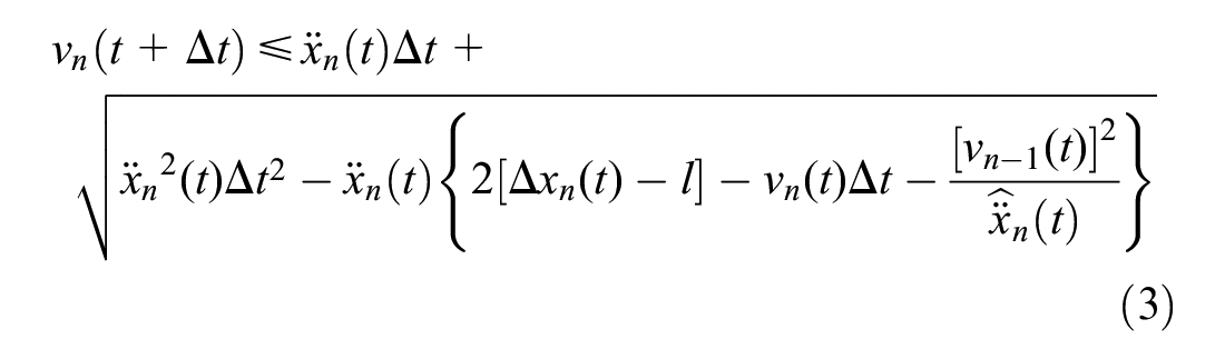
where
Gipps did not use real data to determine the parameters in the model, but assumed that these values are subject to Gaussian distributions.
The above models only consider the relationship between the state of the FV and the closest PV. Factors related to other vehicles (i.e., those preceding the closest PV) are not considered. In the CAV environment, vehicle-to-vehicle communication allows the vehicle to collect information of these vehicles that also affect the car-following behaviors. Besides, the driver factors no longer exist in a pure CAV environment. Thus, to accurately describe the car-following behavior in a CAV system, a car-following model is proposed with the consideration of the joint influences of multiple factors, including vehicle co-optimization velocity, velocity difference of multiple PVs, and the space headways of multiple PVs.
Methods
The Model
Assumptions
In the CAV environment, characteristics related to human drivers, such as reaction time, personal preferences, and driving habits, no longer exist. Therefore, some basic assumptions are introduced:
CAVs operate in a continuous traffic flow facility with a single lane, and thus there is no lane change and overtaking behavior.
CAVs can accurately obtain information in real time, such as the position, velocity, and acceleration of multiple vehicles within a certain distance (related to the sensing distance of the sensing devices installed on and the communication range of CAVs).
No human drivers are involved in the motion control of the vehicle. That is, the driver’s reaction process will not be considered.
Information transmission delay between CAVs is ignored.
Model Formulation
In the CAV environment, information exchange can be achieved among vehicles, and human driver factors can be ignored. Thus, three influence factors in the car-following model are reorganized as follows.
Factor 1: Vehicle co-optimization velocity
The classic optimal velocity function mainly depicts the one-to-one mapping relationship between the desired velocity and the space headway between the FV and the closest PV. However, in the CAV environment, the optimized velocity function is also related to the space headway between the FV and the vehicle following the FV. The speeds of the FV, the closest vehicle following the FV can be cooperatively optimized. This leads to a cooperative velocity optimization function that should be incorporated in the MACF model.
Factor 2: Velocity difference of multiple PVs
In the CAV environment, a vehicle can simultaneously acquire the velocity differences of multiple PVs in a certain range. When the motion state of a PV changes, all vehicles following this PV within a certain distance will receive the information immediately. With the information, the FVs then adjust their accelerations and velocities, so that the traffic flow recovers to the optimal velocity state. To capture this phenomenon, the MACF model should consider the velocity differences between the FV and multiple PVs.
Factor 3: Space headway of multiple PVs
In the actual driving environment, the velocity difference of the two consecutive vehicles is perceived as the change in their space headway. According to Spyropoulou, while pursuing the desired velocity, an FV needs to keep a safety distance from the PV to avoid collisions ( 21 ). This holds for all vehicles preceding the FV being investigated. As a result, the space headways of multiple PVs need to be included as a direct feedback item to build a car-following model for CAVs.
Consider a vehicle indexed as n in a stream of CAVs. Let m be the number of vehicles preceding vehicle n. The value of m is dependent on the sensing distance of the sensors on the vehicle. Further, let i be the index of the i th PV of vehicle n. Note that the PVs are indexed in an ascending order based on their distances to vehicle n.
Combining the three factors mentioned above, the MACF model is formulated as follows.
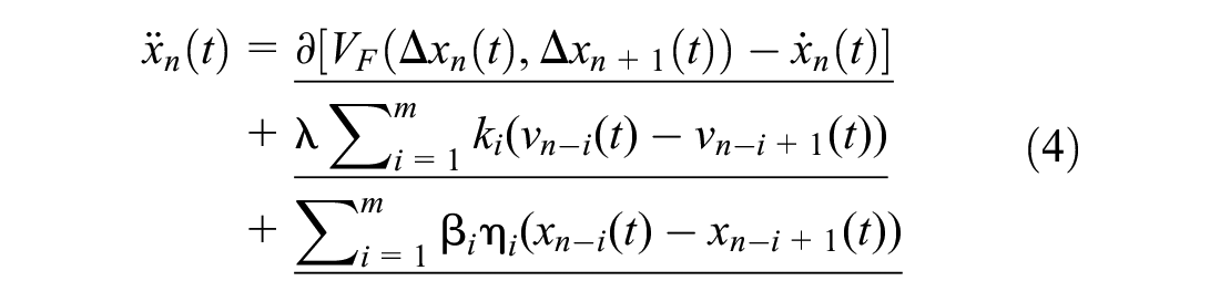
where
In Equation 4, the first, second, and third terms refer to factors 1, 2, and 3 defined above, respectively. Below, the definitions of the key parameters in this model are illustrated.
The cooperative velocity optimization function is formulated as Equation 5:
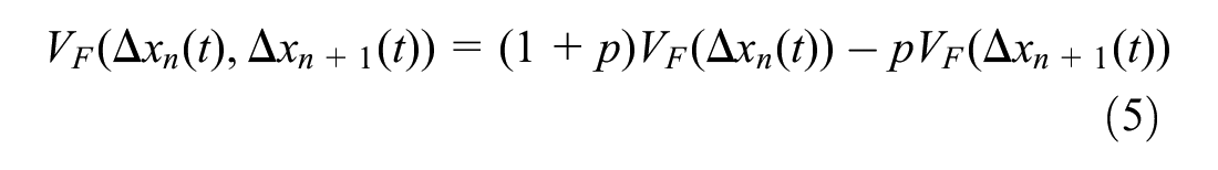
where
p = the smoothing coefficient to coordinate the velocities between different vehicles.
According to Xiao and Gao, and Li et al., the weighting coefficient reflecting the impact of the velocity difference between vehicles

This function reveals that
Finally, The MACF model adopts the space headways of multiple PVs as a direct feedback term. When the headway is greater than the minimum safety distance of the car,
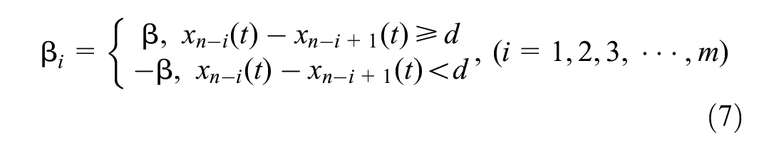
where
d = the minimum safety space headway that can be computed as Equation 8:
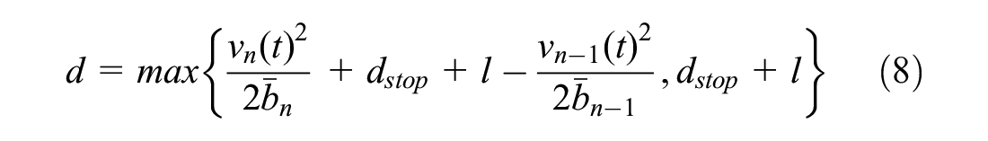
where
Parameter Calibration
In the MACF model, parameters that need to be calibrated include the sensitivity coefficient of the sensors installed on vehicle
Data Source
Since CAVs have not been commonly deployed, it is difficult to obtain large-scale realistic car-following data in an actual CAV environment to calibrate the parameters. To address this issue, a typical solution is to calibrate CAV car-following models with available vehicle trajectory data of HVs. This solution treats HVs as CAVs by assuming that they virtually obtain information of other vehicles and drive autonomously. Note that such information is collected in the HV trajectory data, but in CAV traffic it will be collected via sensors or vehicle-to-vehicle communication. Popularly used is the open source dataset collected for the NGSIM project supported by the U.S. Federal Highway Administration. This dataset has been used to calibrate various CAV models, for example, the velocity control model, the lane-changing model, the cooperative adaptive cruise control, and the collision warning model ( 23 – 26 ). These studies have shown that it is feasible and reasonable to calibrate CAV models with HV trajectory data. Thus, the “US 101 Dataset” from the NGSIM dataset is adopted for model calibration. This dataset contains vehicle travel trajectory data in a research section in the US 101 Expressway from 7:50 to 8:35 a.m. on June 15, 2005. It is divided into three sub-data sets in each 15 min. In each sub-dataset, information includes the attributes (e.g., ID, length, width, type) and trajectories (e.g., time-varying velocity, acceleration, space headway to the PV) for all vehicles traversing the research section within the 15 min. Please refer to Gu for details of the dataset ( 27 ).
Data Preprocessing
The dataset includes trajectory data for vehicles that are not following other vehicles or changing lanes. These data are not applicable to the proposed MACF model, and thus must be removed from the dataset. Additionally, the selected data should also meet the following requirements:
The selected vehicle data should be extracted from the same lane.
Except for the first and last vehicles, all the selected vehicles should have PV and FV.
To ensure that the selected vehicle is in the car-following state, the headway between the PV and FV should not be too long. According to Wang and Chen, the critical headway is 150 ft, which is about 45.72 m ( 28 ).
The selected vehicles are all private cars.
After pre-processing, multiple sets of car-following data on multiple lanes are obtained as the sample data. This produces 150 sample data that could be used for model calibration.
Method and Results
There are mainly two methods for parameter calibration, including the maximum likelihood method and the least squares method ( 29 ). The maximum likelihood method is a statistical estimation method. Thus, the results have statistical characteristics, but partial errors impose biases on global parameter estimations. The least squares method transforms the problem of parameter calibration into optimizing a nonlinear function. This method aims to achieve the smallest global error, and thus the resultant model usually fits the actual data better. This paper adopts the idea of the least squares method to calibrate the parameters in Equation 4.
Instead of using the sum squared absolute error as the objective function as the least squares method, this paper adopts the root mean square error between the estimated acceleration value and the actual value. The root mean square error is formulated as the following Equation 9:

where
N = the number of samples (i.e., vehicles).
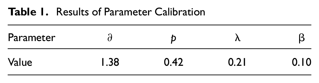
The genetic algorithm in MATLAB is adopted to find the minimum value of Equation 9 ( 30 ). The population size is set as 40, the maximum number of iterations as 200, the crossover probability as 0.6, and the mutation probability as 0.1. The results obtained are shown in Figure 1. It is seen that the algorithm achieves convergence at around the 121st generation, and the optimal fitness value is 6.59. With this, the calibration results of MACF model are obtained as summarized in Table 1:

Convergence curve of calibration process.
Results of Parameter Calibration
Stability Analysis
To further explore whether the MACF model can accurately characterize car-following behavior and evaluate the anti-jamming capability of the traffic flow in a CAV environment, next, the stability of the MACF model is mathematically and numerically investigated. Since the OV model, the FVD model, and the proposed MACF model consider similar factors (e.g., speed difference, optimal velocity), the OV model and the FVD model are used as benchmarks to evaluate the stability of the MACF model mathematically. Besides, the proposed MACF model is compared with the FVD model, the ACC model, and the CACC model via numerical simulation. The FVD model is defined by Equation 2, while the ACC model and the CACC model are from Marsden et al. and Xiao and Gao ( 13 , 14 ).
Theoretical Analysis
Consider a flow of CAVs traveling on a single lane. The vehicles are at a stable state if they travel at a constant velocity and all vehicles have the same headway. In this state, the position of each vehicle can be calculated by Equation 10:

where
n = the vehicle index;
b = the space headway;
At a certain moment, a small disturbance


where
Let


where
The first derivative of Equation 11 is:

The second derivative of Equation 11 is:

From Equations 13 and 14, the following is obtained:


Substituting the Equations 13 to 18 into the MACF model Equation 4, and linearizing the result equation, yields:
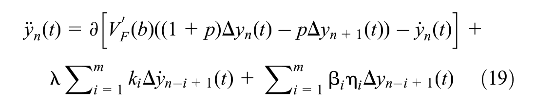
where
Let
Then:


Substituting Equations 20 to 24 into the Equation 19 yields:

To solve Equation 25, the parameter z is expanded to:

Then perform a second-order Taylor expansion on


Then substitute the first two terms of Equations 26, 27, and 28 into Equation 25, and the following is obtained:

Solving Equation 29 gives:

From Equation 30, it is known that, if
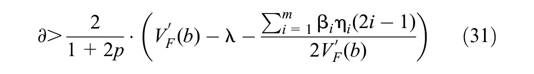
From Equation 31, it is seen that, when

In this case, the MACF model degenerates into the OV model, and stability condition Equation 31 is consistent with the stability condition of the OV model.
When

In this case, the MACF model degenerates into the FVD model, and the stability condition Equation 31 is consistent with the stability condition of the FVD model.
With the above theoretical analysis, the stability curves of the MACF model (
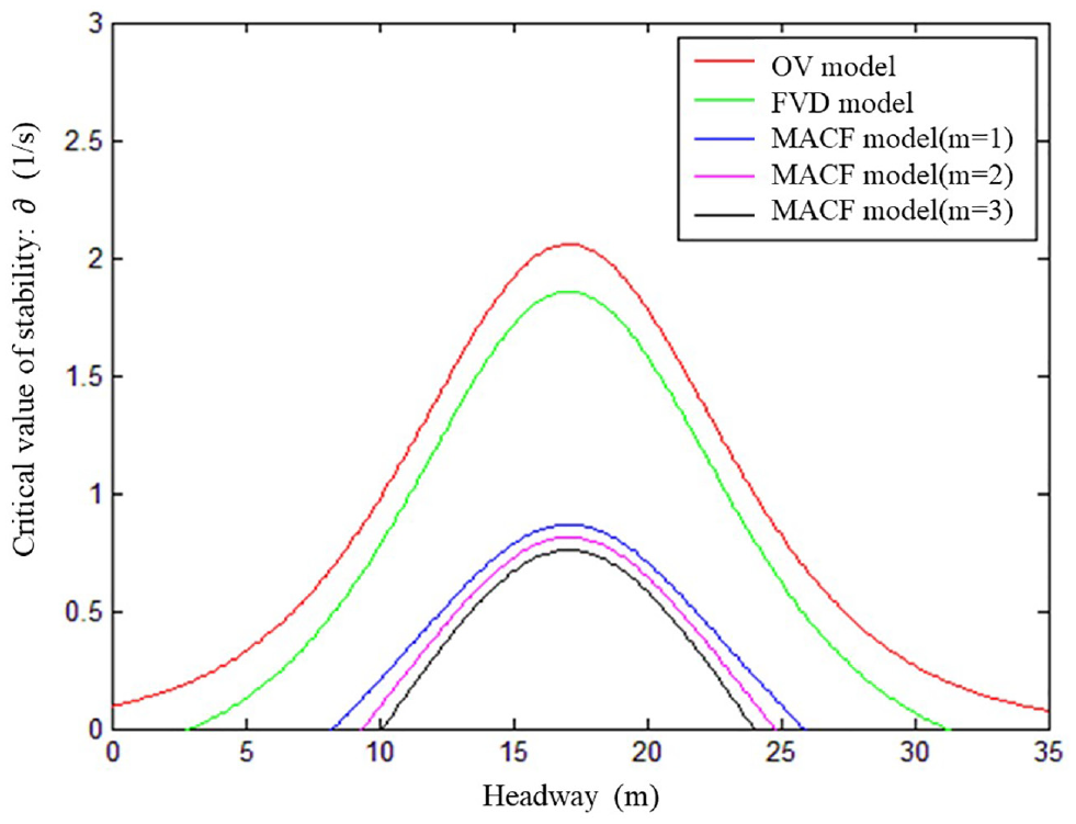
Stability curves of the optimal velocity (OV) model, the full velocity difference (FVD) model and the multiple-factors aware car-following (MACF) models (m = 1,2,3).
It is seen that the stability region of the FVD model is larger than that of the OV model. This is because the FVD model considers the velocity difference between the FV and the closest PV. Besides, the FVD model avoids the unreasonable phenomenon that the vehicle will back up. Further, the stability region of the MACF model is larger than those of both the FVD and the OV model. This improvement is, on one hand, attributed to the consideration of the velocity difference and the space headway of multiple PVs. On the other hand, the optimization velocity function also considers the space headway between the FV and the vehicle following the FW. In addition, it can be seen from Figure 2 that the larger the number of PVs being considered, the stronger the anti-interference ability of the MACF model. Thus, the MACF model is more stable.
Simulation for Stability
To verify the theoretical results of the stability analysis, Jiang et al. are followed, and a virtual loop with a single lane is designed to carry out numerical simulation experiments (
10
). The advantage of this loop setting is that the head vehicle and the tail vehicle can affect each other, and it is convenient to observe the stability of the model. It is assumed that the loop has a length of L =1,500 m. A total number of
Comparison of Vehicle Velocity
Figure 3 shows the velocities of all vehicles at different simulation times based on the MACF model, the FVD model, the ACC model, and the CACC model. First, the MACF model is looked at. When
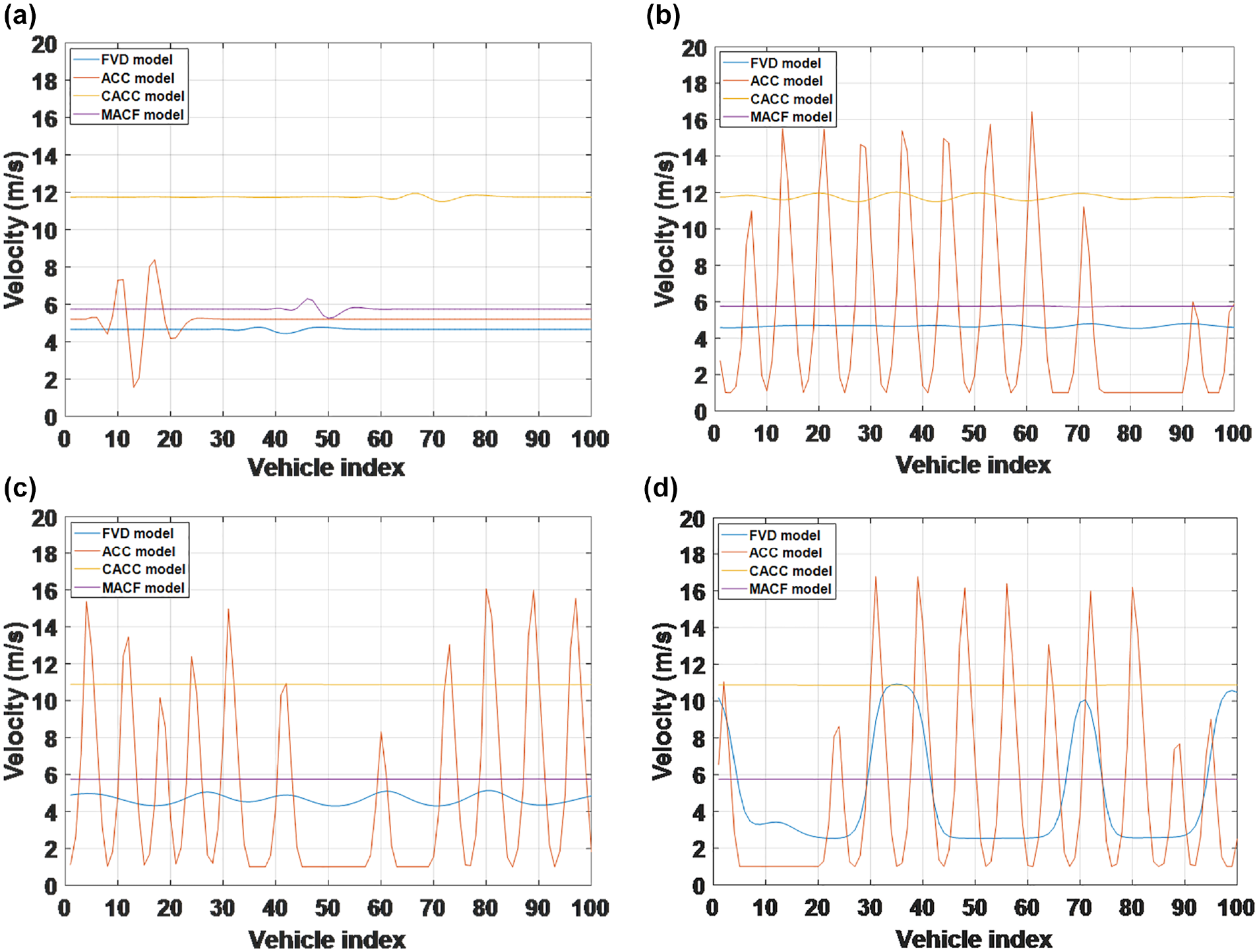
Vehicle velocity distribution at different times simulated by the multiple-factors aware car-following (MACF) model, the full velocity difference (FVD) model, the adaptive cruise control (ACC) model, and the cooperative adaptive cruise control (CACC) model. Vehicles are indexed from 1 to 100 based on their order in the fleet. 100 vehicles are observed at each time index (i.e., sub-figure): (a) t=300s (b) t=900s, (c) t=2000s, and (d) t=4500s.
Moving to the ACC model, when
In summary, the MACF, ACC, and CACC models all respond to the disturbance earlier than the FVD model. The MACF model and the CACC model can both restore the traffic flow to the stable state, but the former can do it more quickly. The FVD model and the ACC model cannot restore the traffic flow to the stable state until the end of the experiment. Therefore, the MACF model can more quickly respond to the disturbance and restore the traffic flow to the stable state compared with the other three selected car-following models.
Comparison of Vehicle Space Headway
Figure 4 presents the space headways between every two consecutive vehicles in the simulation system at different simulation times based on the MACF model, the FVD model, the ACC model, and the CACC model. For the MACF model, similar to the vehicle velocity profile, the influence of the disturbance on the traffic flow gradually dissipates over time. When
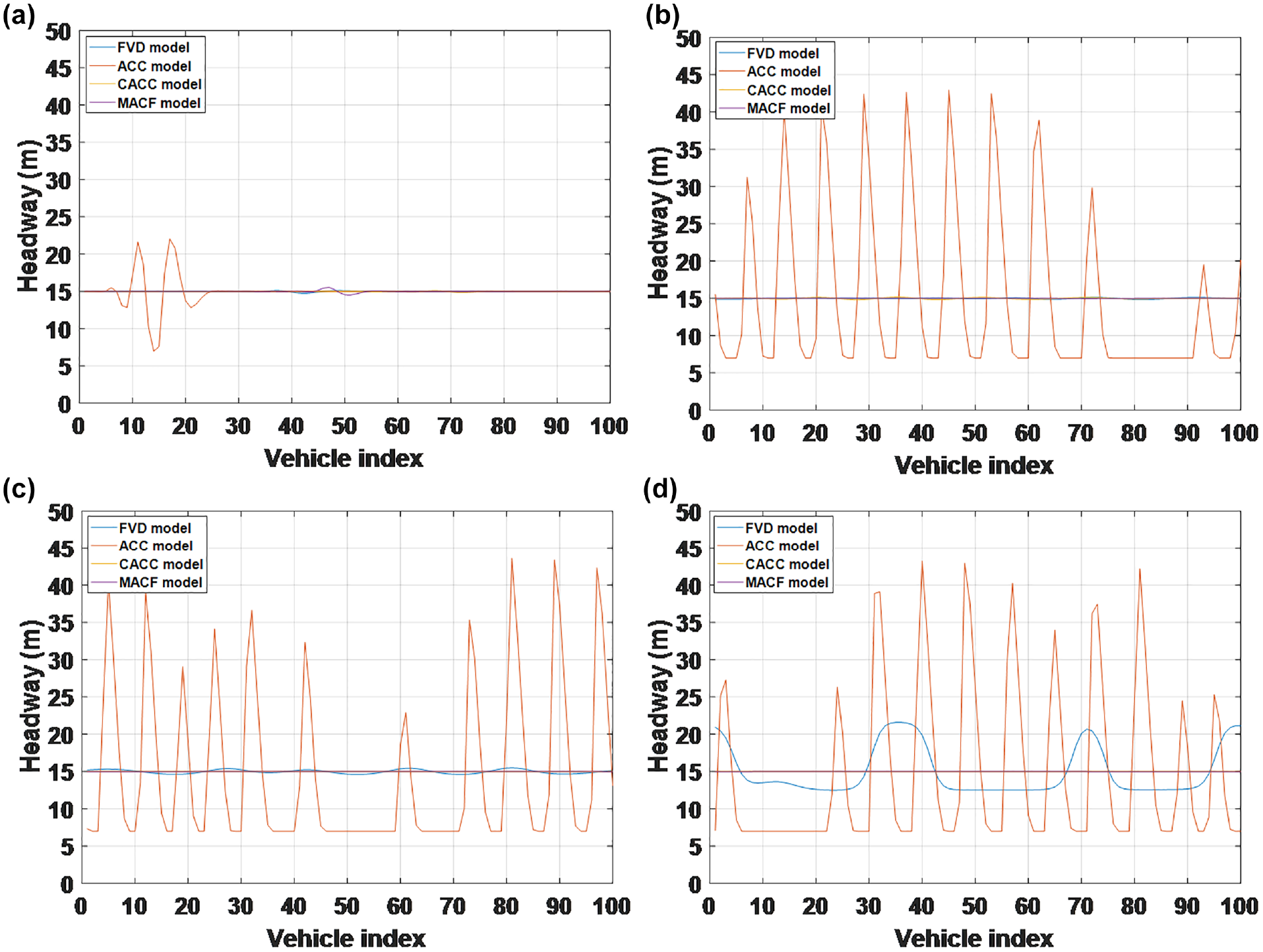
Vehicle space headway distribution at different times simulated by the multiple-factors aware car-following (MACF) model, the full velocity difference (FVD) model, the adaptive cruise control (ACC) model, and the cooperative adaptive cruise control (CACC) model. Vehicles are indexed from 1 to 100 based on their order in the fleet: (a) t=300s, (b) t=900s, (c) t=2000s, and (d) t=4500s.
For the ACC model, all vehicles are affected by the disturbance at
The above results mostly agree with those on the velocity distribution. They also show that the proposed MACF model is faster and can more quickly respond to the disturbance and restore the traffic flow to the stable state compared with the other three selected car-following models.
Comparison of VISSIM Simulation Outputs
Finally, a snapshot of the simulation outcomes from VISSIM at
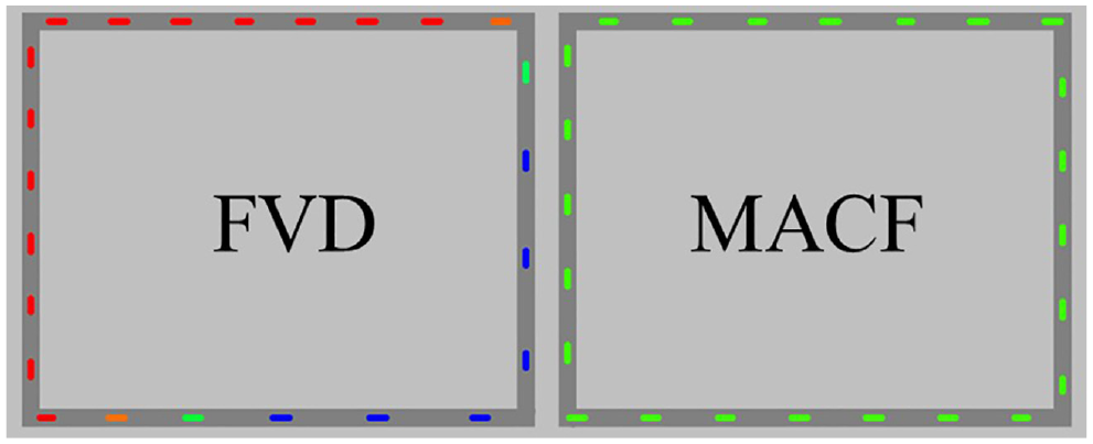
Stability simulation outputs at t = 4500 s simulated by the full velocity difference (FVD) model (left) and the multiple-factors aware car-following (MACF) model (right).
With the above results, it is concluded that the proposed MACF model has better stability than the FVD model. The improvement from modeling the NGSIM data with the MACF model is because the MACF model considers multiple factors that are not present in the FVD model. While the FVD model simply considers the information of the FV and the closest PV, the MACF considers information of the FV and multiple PVs. Information of multiple PVs is not considered in the FVD models because these models are proposed for HVs, which can only obtain information of the closest PV. However, CAVs can obtain information from multiple PVs that is incorporated into the MACF model. This information is collected via sensors and/or vehicle-to-vehicle communication in a CAV environment. Although the NGSIM data do not involve CAVs, the information of multiple PVs is collected. Thus, this information can be informed to the vehicles. As a result, the HVs operate as if they were collecting this information of multiple PVs as CAVs. The multiple factors, as the experiments reveal, do improve the string stability of the traffic flow. However, it is acknowledged that calibrating the proposed MACF model with HV data is limited, as it cannot reflect changes in driving behavior in a CAV environment. Yet, the focus of this paper is to propose a car-following model that considers multiple factors from multiple PVs resulting from the vehicle-to-vehicle communication characteristic of CAVs. It is not intended to propose a model to describe all possible changes brought by CAVs. Thus, it is considered that the simulation approach suffices. However, it would be interesting and meaningful to calibrate the model should trajectory data of CAVs become available in future studies.
Application: Analysis of Mixed Heterogeneous Traffic Flow
As an example application of the proposed MACF model, it is used to simulate a mixed traffic flow consisting of HVs and CAVs in VISSIM. Below, the experiment settings are summarized, and the main results are reported.
Simulation Settings
The simulation considers a single lane with a length of 2.3 km, a width of 3.75 m and a velocity limit of 60 km/h. During the simulation, a new vehicle arrives at the starting point of the road every
Pre-experiments show that, after driving for around 300 m, the traffic flow can almost reach the stable car-following state. Thus, the first 300 m of the road is defined as the buffer district, and the last 1 km is to collect data. The data is collected for 3,600 simulation seconds.
To investigate the impact of CAV proportion on the traffic operation, 11 different proportions (i.e., 0, 0.1, 0.2, 0.3, 0.4, 0.5, 0.6, 0.7, 0.8, 0.9, and 1) are considered. Further, to ensure that the results are representative, 30 simulations are run for each CAV proportion. In each simulation, the HVs and CAVs are randomly mixed. The vehicles are randomly generated as follows. At the beginning of the simulation, a fleet of 100 vehicles indexed from 0 to 99 is generated. Then, A (i.e., the proportion of CAVs) numbers is randomly drawn from 0 to 99. Vehicles with the drawn indexes are then labeled as CAVs. Next, all vehicles are stored in a virtual depot and dispatched to the simulated road every three simulation seconds. A new fleet will be generated and then added to the virtual depot when the depot is close to empty. This procedure is repeated until the end of the simulation. Note that, in the simulation vehicle, platooning effects are not considered, since it would require the design of complicated real-time platooning strategies. This would result in the problem being investigated to a new level of complexity that is out of the scope of this study. Further, average velocity and throughput are used across 30 simulation runs under each CAV penetration rate as the performance metric of the system.
The classic Wiedemann99 model in VISSIM software is selected to model the car-following behavior of HVs. The Wiedemann99 model is a classic “physiological-psychological driving model,” which is a good representation of the car-following state of an HV. The car-following behavior of CAVs are modeled with the proposed MACF model. The specific parameters in both models are calibrated in the previous section.
The experiments are carried out on a computer with a frequency of 3.0 GHz, a processor of I5-7500, and a memory of 8G. Visual C++2019 is used to develop the VISSIM4.3, which includes re-encapsulating the COM components of VISSIM and rewriting the vehicle properties and simulation operation modules, as well as recording and analyzing relevant data. To ensure the controllability and responsiveness, the program is completed by multi-threading technology and asynchronous operation.
Results and Discussions
Figure 6a plots the relationship between average vehicle velocity with the rate of CAVs. Figure 6b plots the relationship between traffic volume and the rate of MACF vehicles.
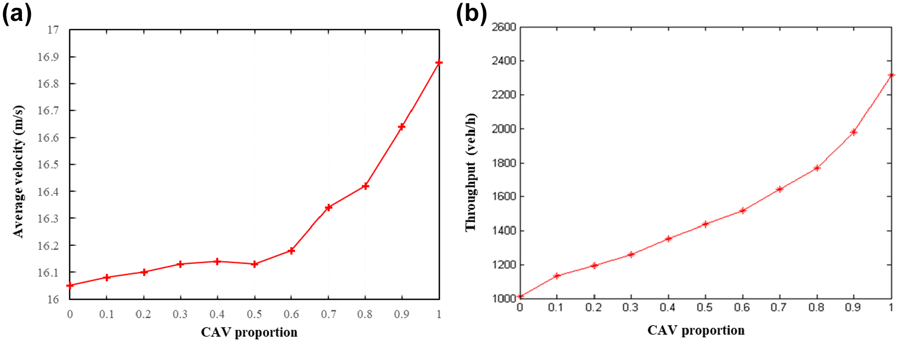
Average vehicle velocity (left) and average throughput (right) with varying connected and autonomous vehicle (CAV) proportion.
Figure 6a shows that the average velocity is at the minimum when the CAV proportion is 0% and gradually increases as the CAV proportion increases. When all vehicles are CAVs (i.e., the CAV proportion is 1), the average velocity reaches a maximum of 16.88 m/s. This result is consistent with the findings in Qu et al. ( 33 ). Further, it is observed that the average velocity increases at a faster rate after the CAV proportion reaches 60%. This is because, when the CAV proportion is less than 60%, HV still accounts for a large proportion of the traffic and thus the interactions between the HVs and CAVs hinder the improvement in system performance. When the CAV proportion is over 60%, the dominance of CAVs in the traffic enables better coordination between the vehicles, which results in a faster growth in the system performance. This result implies that separating HVs from CAVs (e.g., via setting CAV-dedicated lanes) to reduce their interactions may bring better benefits in a mixed traffic system.
In Figure 6b, the throughput of the system exhibits a similar trend. When the ratio of CAVs is 0, the throughput is the smallest (i.e., 1,010 vehicles). As the proportion of CAVs increases, the throughput increases, which is consistent with Yam and Yamamoto ( 34 ). When the proportion of MACF vehicles reaches 60%, the throughput of the system increases at a faster rate, as can be seen by the larger slope of the curve. Finally, when the CAV ratio reaches 100%, the throughput reaches a maximum of 2,318 vehicles, which is 2.3 times that of a 100% HVs.
To sum up, both the average velocity and throughput increases with the ratio of CAVs. This result is consistent with the findings in previous literature, verifying the validity of the proposed MACF model. Further, it shows that the addition of CAVs improves the velocity and throughput in mixed traffic flow.
Conclusion
This paper proposes an MACF model for CAV car-following behaviors. This model jointly considers three unique factors under the CAV environment—vehicle co-optimization velocity, velocity difference of multiple PVs, and the headways of multiple PVs. The NGSIM open source dataset and genetic algorithm are used to calibrate the parameters in the model. Next, theoretical analysis reveals a larger stability domain of MACF model than the traditional OV and FVD models. Numerical simulations using a virtual loop simulation are further conducted to assess the stability of the proposed MACF model, using the FVD model, the ACC model, and the CACC model as benchmarks. Results show that the MACF model quickly restore the traffic flow to the stable state from disturbances, compared with the benchmark models. Finally, the proposed MACF model is incorporated into VISSIM software to showcase the capability of the proposed MACF in studying mixed traffic systems. The results show that the average velocity and throughput in a mixed traffic system increases with the growth in the proportion of CAVs. However, the increase is not linear with the CAV proportion; both the average velocity and throughput increase at a faster rate after the CAV proportion reaches 60%. When society transitions to a pure CAV environment, the velocity and throughput in the transportation system are likely to be 1.05 and 2.3 times that in a pure HV environment. Thus, controlling CAVs based on the MACF model effectively improves the velocity and throughput of mixed traffic flow.
This study can be extended in a few directions. Trajectory data of HVs was used to calibrate the MACF model because of the lack of CAV data during this study. Although a common practice in the literature, it may introduce bias in the parameter estimates, since changes in driving behavior under the CAV environment cannot be captured. Thus, the next step would be to calibrate the model with data from CAVs. In the future, apart from numerical simulations, field experiments can be carried out in the future to verify the performance of the MACF model.
Footnotes
Acknowledgements
The authors would like to thank Professor You Feng at the South China University of Technology for his help in writing this article.
Author Contributions
The authors confirm contributions to the paper as follows: study conception and design: H. Ma, Y. Hu, H. Wu; data collection: H. Wu, J. Luo; analysis and interpretation of results: H. Ma, Y. Hu, Z. Chen, H. Wu; draft manuscript preparation: H. Ma, Y. Hu, H. Wu, Z. Chen, J. Luo. All authors reviewed the results and approved the final version of the manuscript.
Declaration of Conflicting Interests
The author(s) declared no potential conflicts of interest with respect to the research, authorship, and/or publication of this article.
Funding
The author(s) disclosed receipt of the following financial support for the research, authorship, and/or publication of this article: This paper is funded by the National Natural Science Foundation of China: The Research on the Mechanism of Vehicle Safety Coordination Control Based on Vehicle-Vehicle-Road Communication (51108192).