Car Ownership and the Built Environment: A Spatial Modeling Approach

Abstract

Car ownership is linked to higher car use, which leads to important environmental, social and health consequences. As car ownership keeps increasing in most countries, it remains relevant to examine what factors and policies can help contain this growth. This paper uses an advanced spatial econometric modeling framework to investigate spatial dependences in household car ownership rates measured at fine geographical scales using administrative data of registered vehicles and census data of household counts for the Island of Montreal, Canada. The use of a finer level of spatial resolution allows for the use of more explanatory variables than previous aggregate models of car ownership. Theoretical considerations and formal testing suggested the choice of the Spatial Durbin Error Model (SDEM) as an appropriate modeling option. The final model specification includes sociodemographic and built environment variables supported by theory and achieves a Nagelkerke pseudo-R² of 0.93. Despite the inclusion of those variables the spatial linear models with and without lagged explanatory variables still exhibit residual spatial dependence. This indicates the presence of unobserved autocorrelated factors influencing car ownership rates. Model results indicate that sociodemographic variables explain much of the variance, but that built environment characteristics, including transit level of service and local commercial accessibility (e.g., to grocery stores) are strongly and negatively associated with neighborhood car ownership rates. Comparison of estimates between the SDEM and a non-spatial model indicates that failing to control for spatial dependence leads to an overestimation of the strength of the direct influence of built environment variables.

Keywords

planning and analysis transportation demand management policy travel demand modeling transportation planning analysis and application access/accessibility land use and transportation mobility transportation planning policy and processes travel survey methods vehicle classification data public transportation planning and development accessibility model

Cars are ubiquitous in most societies as they offer their users freedom of movement over vast distances. However, the extensive use of cars by a large share of the population is now widely acknowledged to be a leading cause of greenhouse gas emissions responsible for the current climate crisis ( 1 ). It is also linked to negative health impacts through road fatalities and injuries, air pollution and stress ( 2 , 3 ). Car ownership itself is not necessarily perceived as an issue despite the extensive evidence that it is positively associated with higher use of cars and reduced use of other modes, see, for example, Sun et al. ( 4 ), Eluru et al. ( 5 ), Dieleman et al. ( 6 ), Sioui et al. ( 7 ).

Car ownership has been increasing steadily in most countries over the last decades, though there is evidence of a saturation point ( 8 ). In Canada, the number of cars has been increasing 1.8 times faster than the population since 2000. This holds true even in large urban centers. As an example, the number of non-commercial vehicles per 1,000 adults on the Island of Montreal increased by 10% (from 413 to 455) between 2000 and 2018 ( 9 ). This shows how relevant it remains to refine our understanding of car ownership.

Most recent research on the subject has been conducted using disaggregate models where the modeling unit is the household (see the work of Anowar et al. [ 10 ] for a comprehensive review). While those methods allow the researcher to gain insightful knowledge of the mechanism shaping household decisions, they must rely on expensive travel surveys of sometimes small sample sizes, and thus often need complementary survey data from aggregate level datasets. Survey data with sparse spatial distribution could be problematic, for example, when trying to assess the impact of localized changes in transportation infrastructure or accessibility because there might not be enough observations in the zone of influence of those changes. Furthermore, not all regions and cities have access to such detailed travel surveys. Despite some limitations in the interpretability of the data, aggregate modeling can rely on publicly available administrative data or census data where almost all registered vehicles in the studied region can be accounted for. Car ownership rates can thus be estimated at various geographical scales, allowing for a more precise analysis of spatial distribution. A high spatial resolution where the values are aggregated within small geographical units can be useful to investigate the spatial dependence shaping the phenomenon being analyzed.

One measure of spatial dependence is positive spatial autocorrelation, which happens when units that are close to each other present similar values of the investigated variable ( 11 ). This generally means that standard linear models cannot be used because doing this violates the assumptions of independence of observations and uncorrelated error terms. Spatial modeling methods are thus needed to account for and investigate those spatial interactions.

The main objective of this paper is to investigate the relationship between car ownership rates measured within small geographical units and various characteristics of the built environment relevant for transport and planning policy while controlling for spatial dependence.

The investigation starts by testing the hypothesis that the observed spatial correlation in car ownership rates observed at this spatial resolution is explained not only by within-neighborhood sociodemographic and built environment characteristics, but also such characteristics in nearby neighborhoods (i.e., contextual effects). Additionally, because individual transportation decisions have been recognized to be influenced by social interactions ( 12 , 13 ), car ownership decisions of households within a zone could be influenced by the behavior of other households within nearby zones (i.e., endogenous effects), thus potentially affecting the aggregate car ownership rates. This study considers built environment influences such as accessibility to local opportunities, transit and carsharing services. It then examines the impact of not controlling for spatial dependence arising from observed and unobserved factors. To achieve this, a modeling framework is proposed to identify a spatial model specification adequately suited for investigating these questions and to obtain robust estimates of the relationship between car ownership rates and built environment including accessibility. In this respect, aggregate models relying on data covering the entire region allow for precise analysis of the spatial distribution of car ownership and its influencing factors.

Literature Review

Car ownership has been shown to relate to personal and built environment characteristics, and in some cases policy ( 14 ). Age is found to influence car ownership, but not in a linear manner ( 4 ) and some cohorts seem more car-oriented ( 15 ). When modeled at the household level, income is a key determinant in car ownership, with higher income associated with more cars owned even when neighborhood income variables are included instead of household level income ( 16 ). This relationship might not be linear ( 14 , 17 ). Household size has also been shown to positively influence car ownership ( 18 ), as well as household structure such as being a couple or having a child ( 4 , 17 ). The presence of children in the household is not necessarily associated with higher numbers of vehicles when other variables are accounted for ( 19 ).

As to built environment variables, higher residential density or higher mixed density are associated with lower propensity for households to own several cars ( 4 , 17 , 20 ). Some have argued that when attitudes, travel preferences and residential self-selection are accounted for, built environment variables may not be significant factors explaining car ownership ( 21 ), while others have shown that even when controlling for those factors, built environment variables remain significant ( 20 ), even having a direct effect on the household’s car ownership decision ( 22 ).

Related to the built environment are the options provided through the transport network. The impact of transit on car ownership has also been frequently investigated, however with varying levels of precision. Some considered only the number of transit stops accessible within a threshold distance around the household ( 17 ), others added the number of kilometers of bus and rail line within that same buffer ( 16 ). More precise measures describing transit level of service have also been included, showing that higher levels of service are associated with lower car ownership ( 23 ). A lesser investigated, but nonetheless influential variable on car ownership is the availability of on-street and off-street parking in high-density areas, with higher parking availability of both types associated with higher car ownership levels ( 24 , 25 ). This suggests that parking management policies (such as context-based limits) should be used in tandem with the provision of public transportation to reduce the need for car ownership ( 26 ).

As discussed above, built environment features of neighboring areas may influence car ownership, but aggregated spatial modeling methods have rarely been employed to examine car ownership. For example, Clark and Finley ( 27 ) compared three spatial modeling methods—spatial error model (SEM), geographically weighted regression (GWR) and hierarchical Bayesian spatial model—to examine the relationship between household car ownership and income across England and Wales using census data. The modeling unit was electoral wards, with a total of 1,100 units across the country, and the explanatory variables were simply population density and household net income. In another paper, Clark ( 28 ) compared SEM with GWR using the same two variables, but at a finer geographical scale, where a total of 8,000 electoral wards across the country were used. In an exploratory study, Whelan et al. ( 29 ) tested a range of model formulations (linear, log-linear, s-shaped functions such as logistic or Gompertz and GWR) to model the number of cars per adult at the lower layer super output area (LSOA), a UK statistical unit with an average population of 1,500. Numerous sociodemographic variables were included (income, household structure, dwelling tenure, nationality) along with three policy-relevant variables: accessibility by public transport, on-street parking permit cost and coverage, and a measure of local accessibility to amenities. They concluded that all three variables had the expected sign (negative impact on car ownership rates) and magnitude. Except for the GWR formulation, the other models tested by Whelan et al. did not account for spatial autocorrelation. Spatial interaction effects from observed and unobserved factors have also been integrated in discrete choice models of household fleet composition by Paleti et al. ( 30 ). Their results show that a distance-based spatial interaction effect between households is statistically significant, improves model fit and leads to elasticity estimates considerably higher in magnitude than the non-spatial model. This difference in magnitude could lead to very different policy effect forecasts, clearly indicating the need to incorporate spatial dependence when modeling car ownership. Despite this important finding, very few discrete choice models of car ownership in the literature have controlled for spatial dependence in such a way, most likely because of the very complex model estimation requirements. Examining spatial dependence effects is more easily conducted using aggregate models where the entire region is divided into zonal units and car ownership is measured using a continuous outcome variable such as the average number of vehicles per household. A regression model incorporating spatial interaction effects could thus provide us with estimates of the relationship between the influencing factors and car ownership that are robust to the violation of assumption in regression arising from spatial dependence.

The review suggests that advanced state-of-the-art spatial modeling methods, such as the Spatial Durbin Model (SDM) or Spatial Durbin Error Model (SDEM), as suggested by LeSage and Pace ( 31 ) and LeSage ( 32 ), have not been used to model car ownership. Furthermore, previous aggregate car ownership models have been conducted using large geographical units. The smallest reported unit used was the UK’s LSOA ( 29 ) and in the U.S.A., the Transport Analysis Zone ( 33 ). The current paper makes use of administrative data provided by the Province of Quebec (Canada) car registration authority, Société d’assurance automobile du Québec (SAAQ), to model car ownership at a very fine geographical scale using state-of-the-art spatial modeling methods. This allows the use of several sociodemographic and built environment variables to explain local variation in household car ownership rates with the objective of examining the effect of spatial dependence.

As discussed above, various influences on car ownership levels have been found, but the variables considered in spatially aggregated studies have been limited. In this study, the finer grained spatial level allows inclusion of built environment influences at levels that better reflect short walking distances that are key for car-free (or reduced car) life.

Methods

Theoretical Considerations for Spatial Modeling of Car Ownership

Several reasons may explain the presence of spatial dependence where two cases close to each other have similar values (positive spatial autocorrelation) ( 11 ). Three reasons are of high relevance in understanding why car ownership exhibits spatial dependence. The first reason is spatial continuity, where the modeling unit of measurement is smaller than the scale at which the phenomenon varies. In the present case, the modeling unit is the Dissemination Area (DA) of the Canadian census where, on the Island of Montreal, 95% of units have a land area between 0.02 and 0.61 km². The boundaries defined by Statistic Canada for those areas are not specifically designed to model car ownership rates. This means that the size of the modeling unit can be smaller than the scale at which car ownership varies in space.

The second reason is that the spatial autocorrelation of the process being studied depends on the spatial relationship of observed and unobserved influencing factors. The car ownership rate measured within a spatial unit (e.g., census tract) is an aggregation of household behaviors (i.e., the choice of owning one or more cars). As detailed in the previous section, this behavior is influenced by (typically observed) individual and household characteristics (e.g., income, composition, age, education or race) as well as attitudes and lifestyle preferences (usually unobserved). The distribution of those population characteristics across a region, when measured within statistical units, is rarely random and tends to follow spatial distributions that could be the result of forced or self-selection of individuals into specific neighborhoods that fit their preferences or economic constraints. Built environment characteristics such as density, diversity and the type of dwellings are also factors influencing household car ownership decisions, all of which, when measured within spatial units, are likely to exhibit specific patterns of spatial dependence, most likely arising from spatial continuity.

A third important reason leading to spatial dependence is spatial spillover, where car ownership levels in one spatial unit might be influenced not only by conditions in that unit, as described in the previous paragraph, but also by conditions in neighboring units. This could be a result of social norms and interactions between individuals where, for example, car ownership decisions by those within one zone are affected by decisions of individuals within neighboring zones (endogenous effects) ( 34 ). Spatial spillover could also arise from the influence of exogenous conditions in neighboring units. For car ownership, those conditions can be the sociodemographic characteristics of the neighboring zones and, more importantly, the characteristics of the built environment such as density, diversity of land use, design of the streets, presence of local commercial, service or employment opportunities and accessibility to mobility resources such as highways, transit, on-street and off-street parking, carsharing and bikesharing.

Those different explanations for spatial dependence can be modeled by the inclusion of three main types of spatial interactions terms in a regression ( 35 ). Consider a situation where no spatial spillover is taking place and all the known influencing factors of the process being studied are measured. In such a case, a linear regression model with no spatial interaction term could be sufficient to explain all the observed spatial dependence in the dependent variable, leaving no residual spatial correlations, thus respecting the assumption of independent error terms. In reality, it is very likely that one or more influencing factors will be unobserved. Modeling the presence of unobserved spatially correlated variables is commonly achieved by adding a spatial autoregressive coefficient in the error term to reflect the dependence in the regression residuals. A model with only this effect is called an SEM and is defined by the following equation:

\begin{matrix} y = X_{i} β + u \end{matrix}

(1)

\begin{matrix} u = λ W + ε \end{matrix}

(2)

where, using vector notation, for n spatial units W is an n × n matrix where the non-null elements represent spatial units that are connected to each other, β is k × 1 vector of coefficients, λ denotes the average strength of the spatial correlation in the errors and ε is a vector of independently and identically distributed error terms.

The second type of interaction terms allows for the inclusion of endogenous effects arising from social interactions between households and individuals of adjacent zones. Such processes would be modeled through a simultaneous autoregressive model (SAR) where a spatial lag vector is added to the standard linear model that reflects the average value of the neighboring regions’ car ownership rates in explaining a region’s own car ownership level. The equation for the SAR models takes the following form:

\begin{matrix} y = ρ Wy + X β + ε \end{matrix}

(3)

where the parameter ρ represents the strength of the spatial dependence.

The third interaction includes the exogenous (or contextual) spatial spillover effect described above. This process is modeled by a model referred to as the SLX (spatial lag of Xs), which adds the term WXθ where θ is the vector of k × 1 coefficient vector of the lagged X variables to the standard linear model:

\begin{matrix} Y = X β + WX θ + ε \end{matrix}

(4)

While each of these three spatial models includes one type of spatial interaction, the contemporary approach to spatial modeling suggests testing more complex models involving two spatial interaction terms ( 35 ). These models are, first, the SACSAR model (also called the Kelejian-Prucha) which has a spatially lagged dependent variable (WY) and spatially autocorrelated error term (Wε). The second is the SDM, advocated by LeSage and Pace ( 31 ), which includes a lagged dependent variable (WY) and spatially lagged explanatory variables (WX). Finally, the SDEM, suggested by LeSage ( 32 ) as a good option for applied work, is a model with a spatially autocorrelated error term (λW) and spatially lagged independent variables (WX). Not properly modeling those different types of spatial interactions could lead to regression coefficients that are biased and inconsistent.

Model Specification for Small-Scale Aggregate Modeling of Car Ownership

The challenge of determining what model to use is to identifiy which of these possible specifications is best suited to examine the various reasons for the presence of spatial dependence. LeSage and Pace ( 31 ) and, in a later paper LeSage ( 32 ), make the case that the use of the SACSAR model has too many drawbacks for applied work and thus can be ruled out. They suggest that, for most empirical work, only two configurations are left as starting points: SDM and SDEM. Elhorst ( 35 ), referring to LeSage and Pace ( 31 ), indicates that the SDM will offer unbiased coefficient estimates even if the true data generating process is any of the other models (SAR, SEM, SDEM or SACSAR models). Despite this, empirically testing to determine which of SDEM or SDM would be best suited to model the studied phenomenon is not trivial because these two models are not nested. LeSage ( 32 ) suggests that choosing either of those configurations should be based on strong theoretical basis as to the nature of the spatial spillover effects influencing the outcome being studied.

Both models include explicit accounting of contextual neighboring influences through the inclusion of lagged exogenous variables (the Xs). Those lagged variables are usually the average values of the neighbors defined according to the spatial weight matrix. As described above, such influence is likely to be happening in the case of car ownership rates modeled at fine geographical scale. As described by LeSage ( 32 ), exogenous neighborhood effects are considered local spillover effects because there is no feedback mechanism involved. For example, if density increases in zone i, it might only affect car ownership rates in the zones that are first-order neighbors of zone i.

From a theoretical perspective, the main question left to ask to support the selection of either the SDEM or the SDM is whether some endogenous effects could be taking place. As described above, the support for the inclusion of such effect comes from the hypothesis that people’s car ownership decisions would be influenced by the car ownership decisions of their neighbors. This also requires the assumption that “the neighborhood” is considered to be a valid social reference group when it comes to consumption and transport related decisions. Goetzke and Weinberger ( 34 )’s work bring some evidence to this by trying to differentiate between contextual and endogenous effects in car ownership decisions using New York City data. Car ownership rates are first modeled at the block group level and then, in a second step, the estimated values are used as input in a binomial probit model of household car ownership. The endogenous and contextual effects being measured are thus between individual households and their immediate spatial surroundings, that is, the block group of the U.S. Census within which the observed households are located (zones that are very close in size to the DA of the Canadian census used in this paper). The credibility of that assumption of “the neighborhood” as a valid social reference group lies in the scale Goetzke and Weinberger ( 34 ) consider for defining the neighborhood. The block group, like the DA, represents the very streets on which people live. Seeing your neighbor’s cars (or lack of) sitting in their driveway or parked on the street or discussions with your immediate neighbors could affect your own decision. Their paper produced some evidence to support that hypothesis.

In the present case, the modeling unit is the Canadian DA and the “neighborhood” is defined as either the contiguous DA or as the K-nearest DAs (the spatial weight matrix selection methodology is described in the next section). In Montreal’s most central areas, selecting the 30 nearest neighborhoods corresponds roughly to a neighborhood scale of a 12 to 15 min walk. In more suburban areas, this area is larger because of lower density. While it cannot completely be ruled out, the hypothesis in this study is that the endogenous effect is unlikely at this scale. People’s decisions are influenced by social norms, such as how their neighbors behave ( 36 ). However, a household’s decision about how many cars to own (which could be extended to types) is unlikely to be meaningfully affected by the decisions of people living four to eight streets away (10–15 min walk). Evidence from the study of neighborhood networks shows that they rapidly decrease after the first intersection ( 37 ). In other words, the spatial scale of the current analysis would favor the use of the SDEM over the SDM. The SDEM also allows for controlling spatial dependence arising for unobserved influencing factors that are spatially correlated, such as measures of off-street or on-street parking or the attitudes and preferences of people in each DA. For these reasons, the SDEM serves well the objective of investigating the magnitude of the association between car ownership and the built environment at the current scale.

Another consideration supporting this choice is the ease of interpretation of the direct, indirect and total effects. Interpreting those effects is more straightforward for the SDEM than in the case of the SDM. One can simply interpret the regression level coefficients (β_k and θ_k for the lagged exogenous variables): the direct effect is the average influence of the independent variables of zone i on the dependent variable of zone i (β_k). The indirect effect is the average influence of the independent variables of neighboring zones (where the neighboring regions are defined by the row-standardized W matrix, θ_k). This also makes the comparison between the ordinary least-squares (OLS) model , SLX and SDEM coefficients valid ( 35 ), which is an objective of the current paper. On the other hand, the interpretation of the SDM effects relies on simulated direct, indirect and total impacts that are more complex and less intuitive since it has to account for feedback endogenous effects (e.g., Unit A → Unit B → Unit C → Unit A) propagating through the studied region.

A final critical element supporting the choice of the SDEM over the SDM in the current analysis is the inclusion of accessibility variables (sum of transport/commercial opportunities) measured within walking-distance buffers around the centroid of each zone. This method of calculation is common in disaggregate models and offers a very precise estimation of the influence of accessibility using realistic walkable connectivity. It is also more consistent across the region than relying on the number of opportunities within zones of varying size or within varying number of zones, depending on how the spatial weight matrix is specified. However, it implies that the calculation of those variables relies on elements that are not strictly contained within the boundaries of each zone (e.g., the sum of the number of bus stops within 400 m walking buffers of the centroid of zone i would contain some stops from zone i, but also stops located within neighboring zones). For this very reason, those explanatory variables should not be lagged because they already account for neighborhood effects and doing so would result in multiple counting, leading to biased coefficients. While it is possible to choose not to lag some specific exogenous variables, it is not possible to withdraw those variables from the feedback mechanism at play when a lag on the dependent variable is included, such as is the case for the SDM. This would result in multiple counting of the same effects, which could strongly bias the entire regression results.

With exogenous variables being lagged while others are not, the SDEM takes the following form:

\begin{matrix} Y = X β + WX θ + Z ν + u \end{matrix}

(5)

u = λ W + ε

(6)

where X is the vector of independent variables that are lagged and Z the vector of independent variables that are not lagged for the reasons described above. β represents the estimated direct coefficients of the explanatory variables that will be lagged, θ the indirect coefficients of those variables and ν the coefficients of the variables which are not lagged.

Modeling Framework

To examine the hypothesis that the built environment, the transit level of service, and carsharing availability explain part of the spatial dependence and variance in car ownership levels, a cross-sectional spatial modeling framework is proposed. The framework draws extensively from the recent spatial econometric literature and follows closely the procedure described by Elhorst ( 35 ). Elhorst’s framework is a mixture of the modern general-to-specific model specification search strategy recommended by LeSage and Pace ( 31 ) and the more classical specific-to-general strategy set forth by Anselin ( 38 ).

After a proper analysis of the spatial distribution of household car ownership rates and test for spatial autocorrelation using Global Moran’s I test, a linear regression model (OLS) with various sets of potential sociodemographic explanatory variables was run. Anselin (1988)’s Lagrange multiplier tests were used to check if the OLS model should be rejected in favor of either the spatial lag model (SAR) or SEM. As both tests were significant, the SDEM was selected over the SDM for theoretical considerations detailed in the previous sections. Likelihood ratio tests were then conducted to see if this more complex model could be reduced to either the SLX or the SEM. The chosen specification was then tested with varying neighboring structures. LeSage ( 32 )’s fifth principle was used and only simple spatial weight matrices were tested. The selection procedure was based on Stakhovych and Bijmolt’s ( 39 ) recommendation that goodness-of-fit measures and information criteria were good methods to identify a matrix very close to the true specification, especially when the spatial parameter value is high. This sensitivity analysis is also important because Stakhovych and Bijmolt ( 39 )’s findings also indicate that with high values of the spatial parameters (ρ or λ) the regression coefficients could be very sensitive to the weight matrix. While Bayesian model probability was suggested by LeSage and Pace ( 31 ) as able to identify the true specification among very similar matrices, it was deemed unnecessary to try to find the best possible matrix since similar matrices will be highly correlated because of their common elements ( 40 ). Queen’s contiguity matrix, K-nearest neighbors (where K = 10–40, by steps of 5) as well as a matrix of neighbors below threshold distances of 800, 1,000, 1,200, 1,400 and 1,600 m were tested. At this step, the optimal model specification has been confirmed. Candidates for built environment variables (Table 1) were added all at the same time. The objective of adding explanatory variables in two steps was to test if car ownership spatial dependence could be explained only with the inclusion of sociodemographic variables versus also considering the effect of built environment variables. The test procedure for model specification was run again to see if the addition of the built environment variables brought a change to the model specification. Then, each variable was removed one at a time to test if its presence offered a significant improvement to the model fit. Model fit was assessed using Akaike Information Criterion (AIC) values and likelihood ratio test. This step was repeated until no variable could be removed without decreasing significantly the fit of the model.

Table 1.

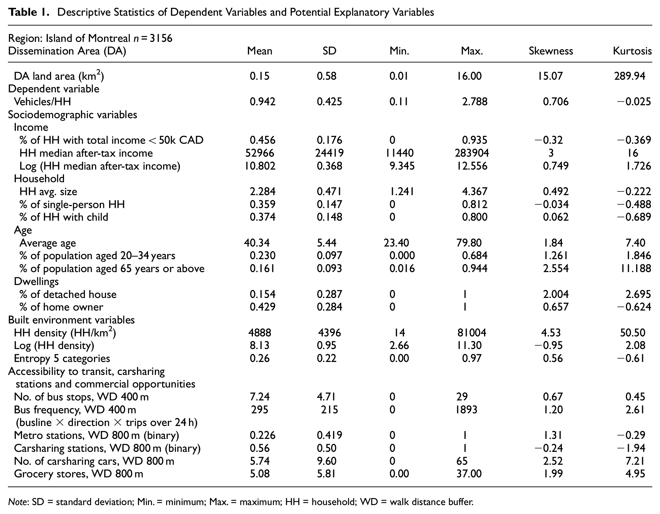
Descriptive Statistics of Dependent Variables and Potential Explanatory Variables

Region: Island of Montreal n = 3156 Dissemination Area (DA)	Mean	SD	Min.	Max.	Skewness	Kurtosis
DA land area (km²)	0.15	0.58	0.01	16.00	15.07	289.94
Dependent variable
Vehicles/HH	0.942	0.425	0.11	2.788	0.706	−0.025
Sociodemographic variables
Income
% of HH with total income < 50k CAD	0.456	0.176	0	0.935	−0.32	−0.369
HH median after-tax income	52966	24419	11440	283904	3	16
Log (HH median after-tax income)	10.802	0.368	9.345	12.556	0.749	1.726
Household
HH avg. size	2.284	0.471	1.241	4.367	0.492	−0.222
% of single-person HH	0.359	0.147	0	0.812	−0.034	−0.488
% of HH with child	0.374	0.148	0	0.800	0.062	−0.689
Age
Average age	40.34	5.44	23.40	79.80	1.84	7.40
% of population aged 20–34 years	0.230	0.097	0.000	0.684	1.261	1.846
% of population aged 65 years or above	0.161	0.093	0.016	0.944	2.554	11.188
Dwellings
% of detached house	0.154	0.287	0	1	2.004	2.695
% of home owner	0.429	0.284	0	1	0.657	−0.624
Built environment variables
HH density (HH/km²)	4888	4396	14	81004	4.53	50.50
Log (HH density)	8.13	0.95	2.66	11.30	−0.95	2.08
Entropy 5 categories	0.26	0.22	0.00	0.97	0.56	−0.61
Accessibility to transit, carsharing stations and commercial opportunities
No. of bus stops, WD 400 m	7.24	4.71	0	29	0.67	0.45
Bus frequency, WD 400 m (busline × direction × trips over 24 h)	295	215	0	1893	1.20	2.61
Metro stations, WD 800 m (binary)	0.226	0.419	0	1	1.31	−0.29
Carsharing stations, WD 800 m (binary)	0.56	0.50	0	1	−0.24	−1.94
No. of carsharing cars, WD 800 m	5.74	9.60	0	65	2.52	7.21
Grocery stores, WD 800 m	5.08	5.81	0.00	37.00	1.99	4.95

Note : SD = standard deviation; Min. = minimum; Max. = maximum; HH = household; WD = walk distance buffer.

Spatial dependence analysis and weighting schemes were conducted using the spdep package in R and spatial models were estimated using the package spatialreg ( 41 , 42 ).

Study Area

The region for the current analysis is the Island of Montreal, Quebec, Canada. It is a subregion of the Greater Montreal Area and it contains the City of Montreal as well as 15 other municipalities. According to the 2016 Canadian Census, the island has a population of 1,942,000 with an average population density of 3,889 persons/km² ( 43 ). In 2016, the transit system had three components: a metro system of four lines and 68 stations (64 located on the Island), a bus system of 218 lines and six lines of commuter trains converging toward the Central Business District. The modeling unit for the analysis is the DA, which is the smallest standard geographical unit for which all census variables are available. This spatial unit is smaller than the U.S. Census Tract, covers all of Canada and has an average population of 400 to 700, based on previous census data. The boundaries of the DA are those of the 2016 census. There is a total of 3,202 DAs on the Island of Montreal among which 3,156 (no missing values in 2016) are considered for the analysis. The unpopulated DAs are mainly parks and industrial areas which are not relevant for an analysis of residential car ownership.

Data Sources

Vehicle Data

The number of residential registered vehicles for 2016 aggregated at the DA level were obtained from SAAQ, the government authority regulating the use of motor vehicles in the Province of Quebec.

Census Variables

A set of sociodemographic variables was obtained from the 2016 Canadian Census at the DA level using the University of Toronto’s CHASS Data Centre.

Built Environment and Accessibility

The land-use dataset was obtained from the Communauté métropolitaine de Montréal (CMM) for the year 2016. The General Transit Feed Specification (GTFS) for 2016 were extracted from Transitfeeds.com. The dataset of carsharing stations was obtained from Communauto, the only station-based carsharing company operating in Montreal. The commercial opportunities were extracted from the Enhanced Point of Interest dataset obtained from DMTI Spatial. The specific extraction procedure can be supplied on demand by the authors. OpenStreetMap’s road and pedestrian network was used for the calculation of walking accessibility buffers. All datasets were integrated in a geospatial database in PostgreSQL, using PostGIS spatial extension.

Preparing the Variables

Dependent variable: The number of vehicles per household was used as the dependent variable. It was obtained by dividing the total number of residential cars and light trucks registered within a DA by the number of private dwellings occupied by residents. It was selected over the number of vehicles per adult because vehicle ownership is mainly a household level decision linked to household disposable income. One limitation of the dataset is that small business owners or people being provided with a company car and who are using these cars also for their personal use are not accounted for since these vehicles are registered as commercial. This would not be a problem if the proportion of such vehicles were distributed homogenously in the region, but this is unlikely to be the case. One assumption is that higher income households are more likely to have vehicles registered this way.

Figure 1 shows a map of the distribution of the number of vehicles per dwelling unit, assuming one household per dwelling in the studied region.

Figure 1.

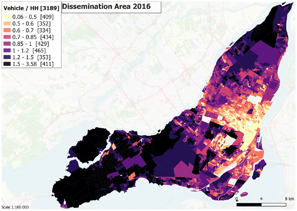
Distribution of vehicles per household on the Island of Montreal at the 2016 dissemination area (DA) level. In the legend, the value between [ ] indicates the number of DAs.

Explanatory variables: All potential sociodemographic and built environment variables (selected based on prior research) are listed in Table 1. The land-use mix entropy within each DA is estimated following the method described by Cervero and Kockelman ( 44 ) considering five land-use categories: residential, commercial, offices, leisure and/or parks, and institutional.

For maximum precision, accessibility to transit and to commercial opportunities were measured as cumulative opportunities within a buffer of space accessible by foot below a threshold distance. Using QGIS’s Network Analysis tool with OSM network accessible by foot (thus including park trails and other pedestrian “shortcuts”), polygons covering the space delimited by a network distance of 400 m and 800 m around the centroid of each DA were calculated. Those distances correspond respectively to about 5 and 10 min of walking at a normal pace. Following tests of association, the 400 m threshold was used for the number of bus stops and a measure of transit level of service: the frequency × direction × bus lines over a period of 24 h. The 800 m buffer was used for the presence of a metro station (binary variable), the number of grocery stores, the number of carsharing vehicles and the presence of at least one carsharing station (again following tests of association for the different thresholds).

While the land area of the dissemination areas is not a potential variable, its presence in the table shows a highly positively skewed distribution because of a few very large areas. In fact, 97.8% of DAs are smaller than the mean plus one standard deviation and the first quartile, median and third quartile values are respectively 0.038, 0.063 and 0.124 km². The log-transform of two highly positively skewed distributions (household median after-tax income and household density) are shown because the transformed variables are used in the models. As the sample size is large (>300), formal normality tests are not recommended ( 45 ). Visual inspection alongside absolute values for skewness (≤2) and of kurtosis (≤7) indicate that most non-binary variables follow a symmetric normal distribution with the exception of the number of carsharing stations and the percentage of the population aged 65 or above.

Results

Moran’s I for the dependent variable (and the null model) shows significant autocorrelation with a value of 0.70 with a row-standardized matrix of 30 nearest neighbors. The value increases to 0.78 when selecting 10 nearest neighbors and decreases to 0.67 when 50 are considered. This indicates that closer neighbors exhibit higher correlation, but the value remains high as the number of neighbors increases.

OLS Models with Sociodemographic Variables

Following the preliminary steps above, which confirmed an important spatial correlation in car ownership rates, several OLS models were estimated with different combinations of variables, one for each sociodemographic sub-category (Table 1). Two sets were retained for further analysis because, as we move through the identification process of the spatial model specification, the set of variables offering the best fit to the data might change. Set A contained four variables: percentage of households with total income of less than $50,000 CAD, percentage of detached houses, percentage of households with a child, and average age. Set B contained five variables: the logarithm of the household median after-tax income, the percentage of home owners, percentage of households with a child, the percentage of the population aged 20 to 34, and the percentage of the population aged 65 or above. In the OLS formulation, Set A with four variables appears to explain more variance, showing better model fit (R² = 0.8664, AIC = −2788.5) than set B with five variables (R² = 0.8411, AIC = −2227.4), and has a lower residuals autocorrelation (Set A: Moran’s I = 0.283, Set B: Moran’s I = 0.36), thus explaining on average across the region more spatial dependence. For both models, however, the studentized Breush–Pagan test values were highly significant indicating important heteroskedasticity.

Spatial Models Results

The Lagrange Multiplier tests for spatial error and spatial lag were conducted on the two OLS models. In both cases, regular and robust tests were all significant at a p-value < 0.0001, clearly indicating that OLS models must be rejected. All test results are reported in Appendix 1. As explained by Golgher and Voss ( 46 ), since all four tests are significant, it does not provide us with clear information on which specification (lag error or lag dependent variable) should be prioritized based on the data generating process.

Following the procedure and theoretical considerations described in the methodology section, a SDEM with lagged exogenous variables and a lag on the error term was estimated for both sets of sociodemographic explanatory variables. Likelihood ratio tests with simpler models (SEM and SLX) were significant, indicating that both models should not be reduced to a model with only one spatial interaction term.

Furthermore, contrary to the OLS formulation, the SDEM specification results indicated that Set B with five variables (M2b: λ = 0.874, LL = 2293, AIC = −4560 and Nagelkerke pseudo-R² of 0.924) presents a better fit to the data than Set A with four variables (M2a: λ = 0.831, LL = 2232, AIC = −4441 and Nagelkerke pseudo-R² of 0.921). This was also the case for the SEM, SAR and SDM specifications. Furthermore, this result holds even when removing either one of the age group variables of Set B. Set B was thus used for the next steps as it offers a better fit to the data when spatial interactions are incorporated.

A first sensitivity analysis for the spatial weight matrix for the SDEM indicates that the structure of 30 nearest neighbors offered the best model fit when only SD variables are included. This step will be repeated on the final formulation of the model.

Adding Built Environment and Accessibility Explanatory Variables

In a first formulation (M3b.1), the following variables were added all at once to the Set B of sociodemographic variables. Two variables were measured within each DA: the logarithm of household density and the entropy for five land-use categories. Four accessibility variables also were measured by a within-walking-distance buffer around the centroid of each DA: the sum of bus stops (400 m), the presence of a metro station (800 m), the sum of local and chain grocery stores (800 m) and the sum of carsharing vehicles within 800 m.

As previously explained, it does not make much sense to have lagged values of those variables as the walking distance buffers already captured neighboring influences. These four variables form the vector Z in Equation 4.

In the first formulation, only the number of carsharing vehicles within an 800 m walking distance radius had a non-significant direct impact. The model was run again (M3b.2), replacing the variable by a dummy variable representing the presence of one or more carsharing stations also within 800 m. This showed a marginal model fit improvement (AIC for M3b.1: −4788.5 versus M3.b.2: −4793.8), the dummy carsharing variable was now significant at p < 0.05 and there was no change in any other variable sign or significance. This could indicate that the presence of carsharing services in the vicinity is important, not the number of stations within reach. A third formulation was run to test if replacing the number of bus stops within 400 m by a measure of transit level of service (the sum of bus line × direction × trips over 24 h accessible at the stops within a 400 m buffer) would improve the fit of the model and better capture the influence of transit on household car ownership rates. This third model formulation (M3b.3) showed a fit improvement (AIC, M3b.2: −4793.8 versus M3b.3: −4821.4) possibly indicating that considering the level of service in addition to the accessibility to bus stops better captures the impact on car ownership rates. A lower value of the λ parameter regulating the strength of the spatial dependence in the error term is also observed (λ, M3b.2: 0.774 versus M3b.3: 0.767) which indicates that more spatial dependence is explained by the included explanatory variables.

Validating the Neighboring Matrix W

Following the recommendations of Stakhovych and Bijmolt ( 39 ), information criterion (AIC) and log-likelihood values were compared for various neighboring structures for this final SDEM specification. Confirming the previous results, a matrix of 30 to 50 nearest neighbors offers the best model fit and thus 30 was selected over larger numbers for simplicity (results of the sensitivity analysis are reported in Appendix 1).

Final Model Results for OLS, SLX and SDEM

The results for the final SDEM specification are presented in Table 2 alongside results for OLS and SLX models. Likelihood ratio tests with the simpler SEM (lagged error term only) and SLX (lagged explanatory variables only) models confirmed that the SDEM is still the best specification. Multicollinearity was assessed using the variance inflation factor (VIF). The average VIF is 2.67 for the included variables and no individual values are above five, ( 47 , 48 ). The highest VIF values are for the log-transform HH Median After-tax income (4.21) and the % of homeowners (4.25). A model without this last variable was tested. The model offered poorer model fit and the changes in the coefficients of built environment and accessibility variables were marginal. Thus the original model was retained. VIF values for the final model are reported in Appendix 1 alongside the matrix or zero-order correlations between variables.

Table 2.

Results for the ordinary least-squares (OLS) model, spatial lag of Xs (SLX) model and Spatial Durbin Error Model (SDEM) specifications for final variable selection

DV = vehicles/100 households	OLS			SLX			SDEM
	β coeff.	SE	p	β coeff.	SE	p	β coeff.	SE	p
(Intercept)	−114.2	15.0	^***	336.8	26.4	^***	111.0	60.9	NS
Direct effect
log(HH Median After-tax income)	20.7	1.36	^***	41.90	1.57	^***	40.21	1.43	^***
% of home owner	43.1	1.77	^***	25.65	1.77	^***	27.05	1.62	^***
% of HH with child	81.6	3.09	^***	49.84	3.64	^***	50.87	3.30	^***
% of pop. aged 20–34	22.6	5.00	^***	32.76	5.39	^***	32.95	4.91	^***
% of pop. aged 65 or above	47.2	4.09	^***	40.29	4.02	^***	40.65	3.67	^***
log(HH density)	−7.3	0.44	^***	−4.00	0.41	^***	−4.29	0.38	^***
Entropy 5 categories	−12.8	1.34	^***	−7.90	1.21	^***	−8.13	1.12	^***
Daily bus frequency, WD 400 m (line × dir. × trips over 24 h)/100	−1.33	0.13	^***	−1.06	0.12	^***	−0.87	0.13	^***
Metro stations, WD 800 m (0/1)	−4.74	0.73	^***	−3.94	0.66	^***	−2.89	0.81	^**
NB of grocery, WD 800 m	−0.77	0.05	^***	−0.35	0.05	^***	−0.30	0.08	^**
Carsharing station, WD 800 m (0/1)	−10.15	0.67	^***	−3.24	0.65	^***	−1.79	0.74	0.02
Indirect effect (lag variables)
log(HH Median After-tax income)	na	na	na	−51.84	2.85	^***	−36.67	5.47	^***
% of home owner	na	na	na	33.33	4.38	^***	34.81	9.05	^**
% of HH with child	na	na	na	33.88	5.89	^***	42.85	12.27	^**
% of pop. aged 20–34	na	na	na	17.45	10.4	0.09	−12.05	19.99	0.55
% of pop. aged 65 or above	na	na	na	45.26	10.3	^***	32.87	19.66	0.09
log(HH density)	na	na	na	−20.33	1.37	^***	−10.75	2.32	^***
Entropy 5 categories	na	na	na	−34.40	4.45	^***	−10.34	7.77	0.18
λ parameter in the error term	na	na	na	na	na	na	0.7671	na	^***
Moran’s I Test for residuals, KN30	0.225	SD = 51	^***	0.154	SD = 35	^***	−0.003	SD = −.54	NS
Nagelkerke pseudo-R²	0.896	na	na	0.920	na	na	0.931	na	na
Log-likelihood	1801	na	na	2215	na	na	2432	na	na
AIC	−3577	na	na	−4391	na	na	−4821	na	na
N	3156	na	na	3156	na	na	3156	na	na
# parameters	14	na	na	20	na	na	21	na	na
Breush–Pagan Test	38.687	DF = 11	^***	42.92	DF = 18	^**	41.78	DF = 18	^*
Likelihood ratio test: SLX/OLS	LR Ratio = 828.23, df = 7, p-value < 2.2e-16					na	na	na	na
Likelihood ratio test: SDEM/SLX	LR Ratio = 432.57, df = 1, p-value < 2.2e-16					na	na	na	na
Likelihood ratio test: SDEM/SEM	LR Ratio = 66.501, df = 7, p-value = 7.5e-12					na	na	na	na

Note: DV has been multiplied by 100 to ease the interpretation of aggregate coefficients; na = not applicable.

p ≤ 0.01

p ≤ 0.001

***

p ≤ 0.0001.

Additionally, the observed spatial spillover and the inconclusivity of the Lagrange Multiplier tests indicate that the presence of social interactions between modeling units (DA) cannot be ruled out. For this reason, the SDM was also run for this final model specification (M3b.3) and the results are available in Appendix 1. The first observation is that the model fits are very similar with the log-likelihood for the SDEM at 2,432 and for SDM at 2,451 and Nagelkerke pseudo-R² values are 0.9305 (SDEM) and 0.9314 (SDM). The second observation is that the strengths of the spatial parameters are also very similar. The parameter lambda for the SDEM is 0.767 and the rho for the SDM is 0.696. With both models being so close to each other, LeSage ( 32 ) indicates that Bayesian posterior model probabilities are needed to identify the true data generating process. For the considerations described in the Methodology section (interpretability of results, issues of double counting for the SDM and theoretical considerations of scale in the social interactions influencing car ownership decisions), the SDEM approach was the preferred model here and results are further analyzed.

Model Results: Controlling for Spatial Dependence

The first observation is that moving from the OLS to the SLX leads to an improvement in model fit as illustrated by the likelihood ratio and the reduction in AIC values, the latter controlling for the addition of the seven new parameters to be estimated. There is also a reduction in residual spatial dependence illustrated by a lower Moran’s I statistic for the residuals. This is a first indication that some of the observed spatial dependence in car ownership rates across the study area could be arising from contextual spillover effects within the 30 nearest neighbors. However, Moran’s test value remains significant (0.154) after controlling for those contextual effects, hinting at the presence of other sources of spatial dependence.

The results of the likelihood ratio (LR) test between the SDEM and SEM (note that only the LR test results are included in the table, not the coefficient and other model statistics of the SEM) indicate that the contextual spillover effects are present even when controlling for spatial dependence from unobserved factors. The LR ratio test between the SDEM and SLX and the high and statistically significant value of the spatial error parameter (λ) confirms the importance of controlling for residual spatial dependence that could arise from unobserved factors. Controlling for both types of spatial dependence results in a superior model fit and uncorrelated SDEM residuals.

One caveat is that, despite adding numerous explanatory variables supported by previous research and taking into consideration spatial autocorrelation through the error term and exogenous variables, the Breusch–Pagan test indicates heteroskedasticity. This is an important limitation because the use of a maximum likelihood estimator is inconsistent in the presence of heteroskedastic disturbance ( 49 ). To palliate this, Kelejian and Prucha ( 49 ) have developed a generalized form of the Generalized Method of Moments (GMM) estimator that allows for heteroskedastic innovation. The method has been implemented in the sphet package made available in R by Piras ( 50 ). The final SDEM specification was thus run again using the function of this package and the results showed minor differences in some of the coefficient estimates. However, all variables had the same sign and the same three indirect effects were not significant (entropy, percentage aged 20–34 and percentage aged 65 or above). The λ parameter is also very similar with a value of 0.752 (versus 0.767 for maximum likelihood). To respect space limitations, the results of this robust heteroskedasticity model are included in Appendix 1.

Results reported in Table 2 show that direct effects of variables included have statistically significant coefficients and all have the expected sign, except possibly for the percentage of population aged 20 to 34, across all three models. Three lagged variables are not significant for the SDEM: Entropy 5 categories, % of pop. aged 20 to 34, and % of pop. aged 65 plus, suggesting that the population age of neighboring areas might not be associated with car ownership within a DA and that the degree of land-use mix beyond each region’s border has no indirect influence beyond what is already captured by other included built environment variables (i.e., lagged household density and the buffer-based accessibility measures such as bus level of service within 400 m or the number of grocery stores within 800 m).

An important observation is the considerable difference in coefficient estimates between the OLS model and the SLX/SDEM because of the inclusion of statistically significant lagged explanatory variables. As for the difference between SLX and SDEM, sociodemographic variables are consistent between the two specifications. However, built environment and accessibility factors show larger differences between estimates, indicating that choosing the wrong model and not accounting for unobserved spatial autocorrelation could bias coefficients and lead to under- or over-estimated effects.

Relationship Between the Built Environment and Accessibility Characteristics on Car Ownership Rate when Controlling for Spatial Dependence

To avoid possible limitations concerning the interpretation of coefficients of aggregated values, sociodemographic characteristics were only used as control variables and are not discussed further, as the main purpose of this paper is to examine the influences on car ownership that could be addressed by city policies. To some extent, one could argue that policies could influence the percentage of households of different types through housing policy, but the focus here is on the transport and land-use influences. As mentioned earlier, with the possible exception of the age variables, all other variables show signs and magnitudes as expected, and thus serve their purpose well. It should be noted that the log-transformed income variable has a positive direct effect, but a negative indirect effect in both the SLX and SDEM. One possible and cautious explanation is the spatial distribution of income across the city where “islands” of wealth are surrounded by low and medium income DAs and vice versa. In those situations, clusters of high disposable income might better support a greater number and diversity of local shops and services, thus decreasing the need to travel far. The relationship between neighborhood income and car ownership rates has also been shown to vary based on density ( 27 , 28 ) or proportion of commuters using public transit ( 51 ). Studying spatial heterogeneity in the relationship between income and car ownership is, however, beyond the scope of the current paper.

To facilitate the appreciation of the relationship between the built environment and accessibility, it is good to keep in mind the distribution of the dependent variable. Across the 3,156 DAs of the Island of Montreal included in the models, the mean rate of car ownership is 94 vehicles per 100 households, with a standard deviation of 42. For the following paragraphs, if no model is specifically mentioned, the coefficients discussed are those of the SDEM.

Density: As expected, both direct and indirect effects of density are negatively associated with car ownership. However, interpreting the density coefficient in the traditional sense of regression might not be advisable because density is usually considered a proxy for a range of other characteristics less commonly observed (e.g., type of housing, parking availability, household composition). This means that it might not be density itself that is responsible for the lower level of car ownership. Furthermore, it cannot be assumed that a change in density affects behavior, or that it can be inferred from the current method. For example, if within a DA an old gas station is replaced by a condominium tower with limited parking per unit, households moving in might own on average fewer vehicles than households already living in the area, thus lowering the average rate of the entire DA. Another reason may relate to higher population densities supporting a wider range of local services, the is, the diversity in local options, that is not captured perfectly by the measures used in this paper. All those possible reasons for why density is negatively associated with car ownership cannot be distinguished using the current framework.

Thus, a cautious interpretation is that, in the current context, for two DAs identical in every aspect except density, the interpretation of the direct effect is that if unit A has a density 10% higher than unit B, it is expected to have a lower car ownership rate, on average, by 0.43 vehicles per 100 households. The indirect effect is that if unit A is surrounded by neighboring DAs with an average household density 10% higher than unit B, then it is expected to have a car ownership rate lower by 1.08 vehicles per 100 households. Both effects combined lead to a total effect of −1.51 vehicles per 100 households if a DA and its surroundings increase in density by 10%. Comparing this effect to the OLS estimate indicates that a model that does not control for spatial dependence could underestimate this effect.

Diversity is measured here using entropy for five categories of land use (residential, commercial, leisure and park, offices and institutional). A value of 0 indicates that the DA contains only one land-use type (residential) and a value of 1 indicates an equal balance of the five land-use types. All else being equal, the direct effect interpretation is that the difference between those two situations is associated with car ownership rates lower by 8.13 vehicles per 100 households. If this seems high compared with other coefficients, changing the diversity of a neighborhood so that the entropy value goes from 0 to 1 is not very realistic. Nonetheless, the results are important as it shows that higher diversity could lead to lower rates of car ownership. However, increasing diversity might require changes to zoning laws in many cities. The entropy measured here is an imperfect measure, and further investigation is needed to assess what combination of land-use categories could support reduced need for car ownership. Results for diversity are consistent with the literature ( 4 ).

Bus accessibility and level of service: On average across the region, a DA that sees an increase of 100 daily bus trips accessible at bus stops within 400 m (5 min of walking) is associated with a reduction of −0.87 vehicles per 100 households. While this might not seem like much, it is important to understand how this unit is calculated and what kinds of changes to bus level of service might lead to an increase of 100 units of this variable. Across the Island of Montreal, the average DA has 7.25 bus stops within 400 m and the average sum of bus trips over 24 h at those bus stops is 295. If one DA is within range of one bus line, with buses running in both directions every 20 min for 16 h per day, the value of this bus level of service variable will be:

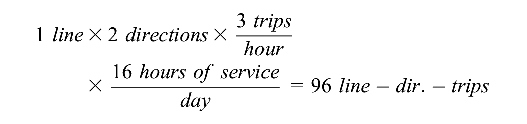
\begin{matrix} 1 line \times 2 directions \times \frac{3 trips}{hour} \\ \times \frac{16 hours of service}{day} = 96 line - dir . - trips \end{matrix}

With this example it becomes easier to interpret the coefficient estimate. Thus, on average in the sample, there are roughly three such lines accessible. If the transit agency was to add three trips/h on this line in both directions (in this case, reducing the headway from 20–10 min), this would be associated with a reduction of 96/100 ×−0.87 = −0.84 vehicles per 100 households for all DAs with centroids located less than 400 m away from the stops of that bus line. Comparing the OLS and the SDEM coefficient indicates that not controlling for spatial dependence could result in slightly overestimating this effect.

Accessibility to a metro station: In the current equilibrium of the studied area, a DA with access to a metro station within 800 m of walking distance (∼10 min at an average walking speed) can expect to have 2.9 vehicles fewer per 100 households compared with a DA identical in all other aspects, but without metro access. It is important to remain cautious in forecasting the impact of adding a metro line using cross-sectional models because such massive infrastructure projects can have complex endogenous effects between built environment, travel behavior and residential self-selection. For example, the opening of a metro line could spur investments in real estate development in the catchment area of that line, leading to an increase in density and diversity, but also a change in the type of housing (the latter of these is not captured in the data used here). The increased accessibility and changes in housing and land use could also lead to important aggregate changes in sociodemographic characteristics arising from population movements (e.g., households with a preference for transit moving close to the new line, lower-income population being forced out, etc.). Like other built environment characteristics, comparing the OLS and the SDEM coefficients indicates that not controlling for spatial dependence results in an overestimation of the association between the presence of a metro station and car ownership.

Station-based carsharing services: Assuming that carsharing is not susceptible to the same complex endogenous effects as metro stations, it is safer to interpret the changes in car ownership rates arising from an increase in accessibility to carsharing vehicles. Holding everything else constant, the SDEM results indicate that adding one station (containing one or more vehicles) within 800 m (∼10 min walk) of DAs which had previously no access, we could expect a reduction of −1.8 vehicles per 100 households. While other methods are needed to assess the causality of the relationship (i.e., are such stations located where people have low access to cars, or is the effect of having such service allowing households to avoid ownership?), the results obtained here are an indication that having access to station-based carsharing services could allow more households to live with fewer cars. The change could come from from self-selection or behavioral change.

Comparing the OLS and SDEM estimated coefficients in Table 2 shows that this variable is one of the most susceptible to controlling for spatial dependence. Failing to do so results in an important overestimation of the effect of carsharing on household vehicle ownership rates.

Local accessibility to grocery stores: The final variable of interest tries to capture the influence of having grocery stores within walking distance. In dense urban neighborhoods, grocery stores do not only consist of large superstores, but can include a myriad of smaller grocery stores. The hypothesis behind the inclusion of this variable was that, as the number of local grocery stores increases, it is more likely that one of the stores will satisfy people’s needs without a car. The exact behavioral mechanism at play cannot be inferred with the current aggregate cross-sectional framework, but results obtained here indicate that from a policy standpoint, increasing access to grocery stores should be further investigated as a possible means to support lower car ownership rates. Across the studied area, the results indicate that an increase of one grocery store within 800 m of walking distance is associated with a value of −0.3 vehicles per 100 households. This might not seem like much, but it is important to understand that one additional grocery store can influence behaviors in several DAs located in its vicinity. Finally, comparing the OLS with the SDEM estimates indicates that without controlling for spatial dependence, this variable would be overestimated.

Discussion and Conclusion

The relationship between household car ownership rates and built environment characteristics is examined in this paper using spatial econometric models that investigate spatial dependence at small geographical units (∼400–700 people) by combining census data with administrative data on registered vehicles. The fine resolution used here (i.e., the DA of the Canadian census) allows for the use of more explanatory variables than previous aggregate models of car ownership. The final formulation produces a Nagelkerke pseudo-R² of 0.93 with coefficients that are robust to the presence of strong spatial dependence. Results indicate that, across all model specifications, built environment characteristics (density, diversity), access to metro stations, bus level of service and station-based carsharing services along with accessibility to local commercial opportunities (grocery stores) are negatively associated with car ownership rates. This confirms previous findings from discrete choice modeling. This also suggests that interventions improving access and level of service of public transportation and accessibility to local opportunities could lead to lower levels of car need and therefore ownership. This agrees with past research indicating that households with fewer vehicles tend to travel less by car in both trips and travel distances (e.g., Sun et al. [ 4 ], Sioui et al. [ 7 ]), supporting the idea that reducing the need for car ownership could lead to reduced car use.

Zonal aggregate data is very useful to investigate the precise spatial distribution of car ownership rates and possible sources of spatial dependence and thus adequately control for the latter. This spatial correlation is something that household-level (disaggregate) data may misrepresent because of sparse sampling in space. A key finding of this paper comes from comparison of coefficient estimates of the OLS model and the SDEM for policy-relevant built environment and accessibility characteristics. The results suggest that not controlling for spatial dependence leads to an overestimation of the direct effect coefficient of all those characteristics, except density. On the other hand, considering the direct and indirect effects of density in the SDEM specification seems to indicate that the ordinary regression underestimates its effect. Additionally, the influence of income (unlike other sociodemographic variables considered), also appears to depend on context.

As for the investigation of sources of spatial dependence, the model inference confirmed that part of it arises from the spatial distribution of sociodemographic and built environment characteristics. Furthermore, testing model specifications with lagged explanatory variables (SLX, SDEM) shows that contextual neighborhood effects also play a role in explaining car ownership spatial dependence. However, the set of included explanatory variables measured within each modeling unit (the DA) and within the larger neighborhood (30 nearest neighbors) could not explain all the spatial correlation still observed in the regression residuals. While the SDEM can produce unbiased coefficient estimates by including a lagged error term that leaves the residuals of the final model clean, the process illustrates that some important spatially correlated variables are currently omitted. Alternatively, some of this unexplained spatial dependence could also arise from social interactions between households of neighboring modeling units. The high similarity in the goodness-of-fit and the strength of the spatial interaction terms between the SDEM (Table 2) and the SDM (Appendix 1) indicate that this possibility could not be ruled out.

Indeed, there is evidence in previous research of social interaction effects in individual and household transportation decisions ( 12 , 13 ), including car ownership decisions ( 34 ), however, those neighborhood interactions most likely fade quickly with distance ( 37 ). As such, the assumption within the current framework was that households within one modeling unit (DA) are unlikely to be influenced by the number of cars owned by households living 10 to 15 walking-minutes away (30 modeling units). Overall, the findings illustrate the importance in future research on car ownership of adequately controlling for spatial dependence from contextual spillover effects and from unobserved factors, confirming previous findings ( 30 , 34 ).

As with all such research, further improvements can be made. The first and most important limitation comes from the aggregate nature of the data and modeling framework. Despite the small size of the modeling unit, the current framework cannot capture the underlying process of household car ownership decisions. While the influence of environmental factors can be assessed on the sum of individual behavior (car ownership rates), controlling for sociodemographic characteristics in the current modeling framework relies on aggregate population measures. This is highly limiting and requires distributional assumptions for those variables that might not be realistic, and thus limit the interpretation of results for those variables.

A second limitation of the findings is that the buffer-based walking distance accessibility measures were calculated from the centroid of each DA, and despite their small size in most of the city, they might not adequately capture the real accessibility experienced by individual households.

An important technical limitation is the presence of heteroskedasticity in the final model specifications, spatial or not, potentially leading to biased coefficients. A potential cause is irregular areal partitioning and variation in population counts of the DAs. However, the results of an estimation procedure for the SDEM that is robust to heteroskedasticity (the GMM estimator) showed minor differences in coefficient estimates, but no change to any variable sign and significance thresholds.

Potential variables that were omitted from this study, whose effects might not be captured by the included variables are: (i) some measures of on-street and off-street parking supply, which have been shown by Guo ( 25 ) to influence car ownership above and beyond the typical income and household characteristics variables; (ii) attitudes toward cars, travel and lifestyle where people of similar thinking tend to cluster in the same neighborhoods ( 22 ); (iii) some measure of job accessibility by transit, by car, by bicycle or some possible combinations of those; (iv) some measure of employment location relative to each modeled DA; (v) the diversity in shop types; (vi) the type and design of infrastructure (e.g., restricting or facilitating high mobility); and (vii) the diversity in housing options. Techniques and data to readily investigate the potential influence of these variables should be explored further. Another important avenue for future research is to expand the current work and the work of Goetzke and Weinberger ( 34 ) to investigate the potential effects of neighborhood social interactions on household car ownership decisions. This should be conducted at a scale at which such interactions are most likely taking place (i.e., the street and street block) using a mixture of household-level data and finely aggregated measures of car ownership.

Additionally, investigating the effect of spatial dependence on car ownership should also consider spatial modeling methods that allow for spatial variation in the strength of the relationship between influencing factors (e.g., income) and car ownership, such as GWR or through the inclusion of spatial regime in the modeling framework. Other spatial resolution(s) should also be tested to assess if the observed impacts of included variables are likely to change, thus leading to different policy recommendations. It would also be highly relevant to validate the results obtained with similar data from other cities and other countries.

Supplemental Material

sj-docx-1-trr-10.1177_03611981211049409 – Supplemental material for Car Ownership and the Built Environment: A Spatial Modeling Approach

Supplemental material, sj-docx-1-trr-10.1177_03611981211049409 for Car Ownership and the Built Environment: A Spatial Modeling Approach by Jerome Laviolette, Catherine Morency, Owen D. Waygood and Konstadinos G. Goulias in Transportation Research Record

Footnotes

Acknowledgements

The authors would like to acknowledge the extensive comments received from two anonymous reviewers for TRR that strongly contributed to enhancing the quality of this paper and the reviewers of the version submitted for presentation at the Transportation Research Board Annual Meeting in January 2021.

Author Contributions

The authors confirm contribution to the paper as follows: study conception and design: J. Laviolette, C. Morency, O. D. Waygood, and K. G. Goulias; data collection: J. Laviolette; analysis and interpretation of results: J. Laviolette, C. Morency, O. D. Waygood, K. G. Goulias; draft manuscript preparation: J. Laviolette, O. D. Waygood, C. Morency, and K. G. Goulias. All authors reviewed the results and approved the final version of the manuscript.

Declaration of Conflicting Interests

The author(s) declared no potential conflicts of interest with respect to the research, authorship, and/or publication of this article.

Funding

The author(s) disclosed receipt of the following financial support for the research, authorship, and/or publication of this article: Funding was provided by the partners of Polytechnique Montréal Mobility Chair and Chair on Transportation Transformation, by the Fond de Recherche nature et technologie du gouvernement du Québec (FRQNT) and by the CIRRELT. The authors would like to thank the Société d’assurance automobile du Québec (SAAQ) for providing on request the main dataset for this study. The first author wishes to thank the GeoTrans Lab at the University of California Santa Barbara for the collaboration that made this study possible.

ORCID iDs

Jerome Laviolette

Catherine Morency

Owen D. Waygood

Konstadinos G. Goulias

Supplemental Material

Supplemental material for this article (Appendix 1) is available online.

References

The Intergovernmental Panel on Climate Change. Transport. In Climate Change 2014: Mitigation of Climate Change. Contribution of Working Group III to the Fifth Assessment Report of the Intergovernmental Panel on Climate Change. IPCC, Cambridge, UK and New York, 2014.

The World Bank. Transport for Health: The Global Burden of Disease from Motorized Road Transport. In Global Road Safety Facility. The World Bank: Institute for Health Metrics and Evaluation, Seattle, WA, 2014.

Nieuwenhuijsen

Bastiaanssen

Sersli

Waygood

E. O. D.

Khreis

Implementing Car-Free Cities: Rationale, Requirements, Barriers and Facilitators. In Integrating Human Health into Urban and Transport Planning: A Framework, Springer International Publishing, Cham, 2019, pp. 199–219.

Sun

Y.-L.

Susilo

Y. O.

Waygood

E. O. D.

Wang

D.-H.

Detangling the Impacts of Age, Residential Locations and Household Lifecycle in Car Usage and Ownership in the Osaka Metropolitan Area, Japan. Journal of Zhejiang University Science A, Vol. 15, No. 7, 2014, pp. 517–528.

Eluru

Pinjari

Pendyala

Bhat

An Econometric Multi-Dimensional Choice Model of Activity-Travel Behavior. Transportation Letters, Vol. 2, No. 4, 2010, pp. 217–230.

Dieleman

F. M.

Dijst

Burghouwt

Urban Form and Travel Behaviour: Micro-level Household Attributes and Residential Context. Urban Studies, Vol. 39, No. 3, 2002, pp. 507–527.

Sioui

Morency

Trépanier

How Carsharing Affects the Travel Behavior of Households: A Case Study of Montréal, Canada. International Journal of Sustainable Transportation, Vol. 7, No. 1, 2013, pp. 52–69.

Davis

S. C.

Boundy

R. G.

Transportation Energy Data Book: Edition 37.2. Oak Ridge National Laboratory, Oak Ridge, TN, 2019.

Laviolette

Morency

Waygood

E. O. D.

Persistance de l’automobilité ? Analyse en trois perspectives. Flux, Vol. 119–120, No. 1, 2020, pp. 142–172.

10.

Anowar

Eluru

Miranda-Moreno

L. F.

Alternative Modeling Approaches Used for Examining Automobile Ownership: A Comprehensive Review. Transport Reviews, Vol. 34, No. 4, 2014, pp. 441–473.

11.

Haining

R. P.

Spatial Autocorrelation. In International Encyclopedia of the Social & Behavioral Sciences, Pergamon, Oxford, 2001, pp. 14763–14768.

12.

Dugundji

Páez

Arentze

Social Networks, Choices, Mobility, and Travel. Environment and Planning B: Planning and Design, Vol. 35, No. 6, 2008, pp. 956–960.

13.

Dugundji

E. R.

Páez

Arentze

T. A.

Walker

J. L.

Carrasco

J. A.

Marchal

Nakanishi

Transportation and Social Interactions. Transportation Research Part A: Policy and Practice, Vol. 45, No. 4, 2011, pp. 239–247.

14.

Senbil

Kitamura

Mohamad

Residential Location, Vehicle Ownership and Travel in Asia: A Comparative Analysis of Kei-Han-Shin and Kuala Lumpur Metropolitan Areas. Transportation, Vol. 36, No. 3, 2009, pp. 325–350.

15.

Sun

Y.-L.

Waygood

E. O. D.

Huang

Do Automobility Cohorts Exist in Urban Travel? Case Study of Osaka Metropolitan Area, Japan. Transportation Research Record: Journal of the Transportation Research Board, 2012. 2323: 18–24.

16.

Anowar

Eluru

Miranda-Moreno

L. F.

Analysis of Vehicle Ownership Evolution in Montreal, Canada Using Pseudo Panel Analysis. Transportation, Vol. 43, No. 3, 2016, pp. 531–548.

17.

Potoglou

Kanaroglou

P. S.

Modelling Car Ownership in Urban Areas: A Case Study of Hamilton, Canada. Journal of Transport Geography, Vol. 16, No. 1, 2008, pp. 42–54.

18.

Kim

H. S.

Kim

Effects of Public Transit on Automobile Ownership and Use in Households of the USA. Review of Urban & Regional Development Studies, Vol. 16, No. 3, 2004, pp. 245–262.

19.

Bhat

C. R.

Pulugurta

A Comparison of Two Alternative Behavioral Choice Mechanisms for Household Auto Ownership Decisions. Transportation Research Part B: Methodological, Vol. 32, No. 1, 1998, pp. 61–75.

20.

Bhat

C. R.

Guo

J. Y.

A Comprehensive Analysis of Built Environment Characteristics on Household Residential Choice and Auto Ownership Levels. Transportation Research Part B: Methodological, Vol. 41, No. 5, 2007, pp. 506–526.

21.

Cao

Mokhtarian

P. L.

Handy

S. L.

Cross-Sectional and Quasi-Panel Explorations of the Connection Between the Built Environment and Auto Ownership. Environment and Planning A: Economy and Space, Vol. 39, No. 4, 2007, pp. 830–847.

22.

Van Acker

Mokhtarian

P. L.

Witlox

Car Availability Explained by the Structural Relationships Between Lifestyles, Residential Location, and Underlying Residential and Travel Attitudes. Transport Policy, Vol. 35, 2014, pp. 88–99.

23.

Becker

Loder

Schmid

Axhausen

K. W.

Modeling Car-Sharing Membership as a Mobility Tool: A Multivariate Probit Approach with Latent Variables. Travel Behaviour and Society, Vol. 8, 2017, pp. 26–36.

24.

Guo

Does Residential Parking Supply Affect Household Car Ownership? The Case of New York City. Journal of Transport Geography, Vol. 26, 2013, pp. 18–28.

25.

Guo

Residential Street Parking and Car Ownership. Journal of the American Planning Association, Vol. 79, No. 1, 2013, pp. 32–48.

26.

De Gruyter

Truong

L. T.

Taylor

E. J.

Can High Quality Public Transport Support Reduced Car Parking Requirements for New Residential Apartments?

Journal of Transport Geography, Vol. 82, 2020, p. 102627.

27.

Clark

Finley

Spatial Modelling of Car Ownership Data: A Case Study from the United Kingdom. Applied Spatial Analysis and Policy, Vol. 3, No. 1, 2009, pp. 45–65.

28.

Clark

Estimating Local Car Ownership Models. Journal of Transport Geography, Vol. 15, No. 3, 2007, pp. 184–197.

29.

Whelan

Crockett

Vitouladiti

A New Model of Car Ownership in London: Geo-Spatial Analysis of Policy Interventions. Proc., European Transport Conference, Glasgow Scotland, UK, 2010.

30.

Paleti

Bhat

C. R.

Pendyala

R. M.

Goulias

K. G.

Modeling of Household Vehicle Type Choice Accommodating Spatial Dependence Effects. Transportation Research Record: Journal of the Transportation Research Board, 2013. 2343: 86–94.

31.

LeSage

J. P.

Pace

R. K.

Introduction to Spatial Econometrics. Chapman and Hall/CRC, New York, 2009.

32.

LeSage

J. P.

What Regional Scientists Need to Know about Spatial Econometrics. SSRN, 2014. https://dx-doi-org.web.bisu.edu.cn/10.2139/ssrn.2420725.

33.

Holtzclaw

Clear

Dittmar

Goldstein

Haas

Location Efficiency: Neighborhood and Socio-Economic Characteristics Determine Auto Ownership and Use - Studies in Chicago, Los Angeles and San Francisco. Transportation Planning and Technology, Vol. 25, No. 1, 2002, pp. 1–27.

34.

Goetzke

Weinberger

Separating Contextual from Endogenous Effects in Automobile Ownership Models. Environment and Planning A: Economy and Space, Vol. 44, No. 5, 2012, pp. 1032–1046.

35.

Elhorst

J. P.

Applied Spatial Econometrics: Raising the Bar. Spatial Economic Analysis, Vol. 5, No. 1, 2010, pp. 9–28.

36.

Nolan

J. M.

Schultz

P. W.

Cialdini

R. B.

Goldstein

N. J.

Griskevicius

Normative Social Influence Is Underdetected. Personality and Social Psychology Bulletin, Vol. 34, No. 7, 2008, pp. 913–923.

37.

Grannis

From the Ground Up: Translating Geography into Community Through Neighbor Networks. Princeton University Press, Princeton NJ, 2009.

38.

Anselin

Spatial Econometrics: Methods and Models. Springer, Dordrecht, 1988.

39.

Stakhovych

Bijmolt

T. H. A.

Specification of Spatial Models: A Simulation Study on Weights Matrices. Papers in Regional Science, Vol. 88, No. 2, 2009, pp. 389–408.

40.

LeSage

J. P.

Pace

R. K.

The Biggest Myth in Spatial Econometrics. Econometrics, Vol. 2, No. 4, 2014, pp. 217–249.

41.

Bivand

Package ‘spatialreg’ : Spatial Regression Analysis. https://cran.r-project.org/web/packages/spatialreg/spatialreg.pdf.

42.

Bivand

Package ‘spdep’ : Spatial Dependence: Weighting Schemes, Statistics. https://cran.r-project.org/web/packages/spdep/spdep.pdf.

43.

Statistic Canada. Montréal, TÉ [Census division], Quebec and Quebec [Province] (Table). Census Profile. Ottawa. https://www12.statcan.gc.ca/census-recensement/2016/dp-pd/prof/index.cfm?Lang=E. Accessed July 23, 2020.

44.

Cervero

Kockelman

Travel Demand and the 3Ds: Density, Diversity, and Design. Transportation Research Part D: Transport and Environment, Vol. 2, No. 3, 1997, pp. 199–219.

45.

Kim

H.-Y.

Statistical Notes for Clinical Researchers: Assessing Normal Distribution (2) Using Skewness and Kurtosis. Restorative Dentistry & Endodontics, Vol. 38, No. 1, 2013, pp. 52–54.

46.

Golgher

A. B.

Voss

P. R.

How to Interpret the Coefficients of Spatial Models: Spillovers, Direct and Indirect Effects. Spatial Demography, Vol. 4, No. 3, 2016, pp. 175–205.

47.

Field

Miles

Field

Discovering Statistics Using R. SAGE Publications, London, UK. 2012.

48.

Dormann

C. F.

Elith

Bacher

Buchmann

Carl

Carré

Marquéz

J. R. G.

Gruber

Lafourcade

Leitão

P. J.

Münkemüller

McClean

Osborne

P. E.

Reineking

Schröder

Skidmore

A. K.

Zurell

Lautenbach

Collinearity: A Review of Methods to Deal with it and a Simulation Study Evaluating Their Performance. Ecography, Vol. 36, No. 1, 2013, pp. 27–46.

49.

Kelejian

H. H.

Prucha

I. R.

Specification and Estimation of Spatial Autoregressive Models with Autoregressive and Heteroskedastic Disturbances. Journal of Econometrics, Vol. 157, No. 1, 2010, pp. 53–67.

50.

Piras

sphet: Spatial Models with Heteroskedastic Innovations in R. Journal of Statistical Software, Vol. 35, No. 1, 2010, pp. 1–21.

51.

Trendle

Public Transport Access and its Implications for Household Car Ownership: A Case Study of the Sydney Greater Metropolitan Area. Australasian Journal of Regional Studies, Vol. 25, No. 2, 2019, pp. 196–222.

Supplementary Material

Please find the following supplemental material available below.

For Open Access articles published under a Creative Commons License, all supplemental material carries the same license as the article it is associated with.

For non-Open Access articles published, all supplemental material carries a non-exclusive license, and permission requests for re-use of supplemental material or any part of supplemental material shall be sent directly to the copyright owner as specified in the copyright notice associated with the article.

0.00 MB

0.09 MB