Review of Length Approximations for Tours with Few Stops

Abstract

The shortest tour distance for visiting all points exactly once and returning to the origin is computed by solving the well-known traveling salesman problem (TSP). Owing to the large computational effort needed for optimizing TSP tours, researchers have developed approximations that relate the average length of TSP tours to the number of points, n, visited per tour. The existing approximations are used in transportation system planning and evaluation for estimating the distance for vehicles with large capacities (e.g., delivery trucks) where n is relatively large. However, the average TSP tour lengths would be inaccurately estimated if the approximations were derived for a wide range of n values since the tour lengths increase at a decreasing rate (i.e., with $\sqrt{n}$ ) as n increases. A comprehensive review is presented here of existing studies approximating TSP tour lengths for low n values, which have become important for some recently favored delivery alternatives (e.g., deliveries by bikes, drones, and robots).

Keywords

traveling salesman problem tour length approximation transportation analysis transportation planning method

The shortest tour distance for visiting all n points exactly once and returning to the origin is computed by solving the well-known traveling salesman problem (TSP) ( 1 ). This problem belongs to the class of NP (nondeterministic polynomial)-hard problems in which finding the optimal path requires computation time that increases exponentially with the number of points, n ( 2 , 3 ). Owing to this large computational effort, researchers have developed approximations for the relation between the average length of TSP tours and n values. Since the distance approximation models are capable of analyzing complex transportation systems reasonably well, the approximations have been used in various transportation planning and system design applications, such as for public transportation services, facility location, and fleet sizing (Figure 1) ( 2 ).

Figure 1.

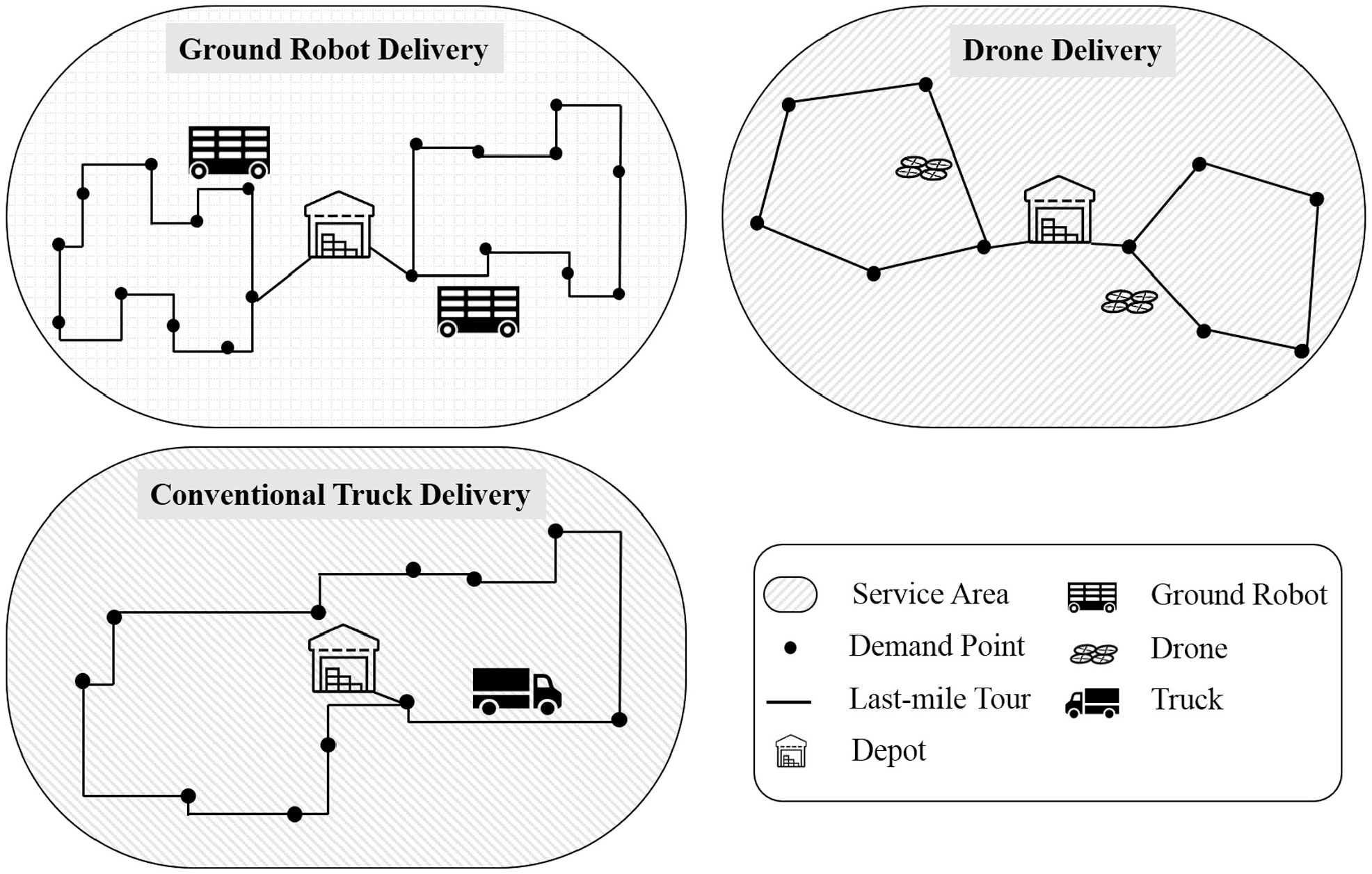
Some examples of delivery tours to a few points.

An approximation provides useful estimates and insights to operators and researchers who seek to reduce costs or improve system efficiency in large-scale problems. However, the approximation models estimated for a wide range of n tend to inaccurately approximate the average tour length if n, that is, the number of points served, is relatively small; the approximation coefficient, β, asymptotically approaches a specific value when n approaches infinity. The “small”n value (i.e., few stops) could be subjective depending on the intended applications. This study chose to emphasize small n values since approximations that seek to cover large ranges of n, possibly to infinity, tend to yield poorer results for the small n values needed in many practical applications, such as flexible-route passenger services (e.g., carpool, dial-a-ride, and airport shuttle [4, 5]), deliveries of large items (e.g., large household appliances), deliveries by robotic vehicles with small capacity (e.g., drones), deliveries by environmentally friendly vehicles (e.g., bike deliveries [6]), or tours by service and repair workers.

Even for vehicles with a large capacity (i.e., trucks), Holguín-Veras and Patil showed that more than 50% of truck routes had fewer than six stops, whereas 95% of the truck routes had fewer than 20 stops in Denver, CO ( 7 ). Although these types of vehicles may not handle economically many shipments per tour, new businesses adopting new technologies have grown because of their advantages, which include speed, responsiveness, and freshness for some items. Therefore, the tour length for these transportation alternatives may not be reliably approximated. The approximations for few n points are promising for analyzing new types of vehicles and delivery alternatives because actual tours serve relatively few customers, particularly with vehicle loading capacity or working period constraints.

This study summarized existing studies in (1) approximation methods for TSP tour lengths with relatively low n values and (2) experimental settings for obtaining TSP tour length approximations. After existing studies on approximations are explored, solution methods for deriving the approximations are explained. That includes experimental procedures, such as the generation of visited points, solution algorithms/heuristics, and estimation methods (e.g., ordinary least squares [OLS] regression and neural network). From the review, the gaps in the current knowledge and possible improvements in approximation models are identified.

Literature Review

This study chose to emphasize small n values because approximations that seek to cover large ranges of n, possibly to infinity, tend to yield poorer results for the small n values in many practical applications, such as flexible-route passenger services, deliveries of large items (e.g., large household appliances), deliveries by robotic vehicles with small capacity (e.g., drones), or tours by service and repair workers.

The study selectively reviewed 22 papers approximating TSP tour lengths with low n values and seven papers were chosen for their experimental approaches or solution methods. Excluded from the approximation studies were (1) those dealing solely with many points (i.e., n > 100) and (2) those that applied rather than developed approximation methods. However, the study did include a few research activities discussing large n values if the research pioneered the field or was worth mentioning for its experiments. For experimental approaches, the study focused on comparing solution methods.

Overview of Average TSP Tour Length Approximation

Approximations for the TSP Tour Lengths

The average distance between two points in both Euclidean and rectilinear space can be mathematically derived. Here, the Euclidean space allows vehicle movements in straight lines between any pair of points, whereas rectilinear space refers to movements that are restricted to two orthogonal coordinates. Although an average TSP distance with three points could still be analytically computed, estimating the tour lengths becomes challenging as the number of points, n, increases.

In early studies of distance approximation models, Mahalanobis suggested that average TSP tour lengths for visiting a set of points, n, in a region served by a single vehicle asymptotically converged to $\sqrt{n}$ with large n, where the points, n, were scattered at random within the space ( 8 ). Later, Marks mathematically proved the approximation by providing a lower bound for the expected value of the distance, as shown in Equation 1 ( 9 ),

Average TSP Tour Length ≅ β \sqrt{\frac{A}{2}} \frac{n - 1}{\sqrt{n}}

(1)

where β is a coefficient and A is the zone size.

With a large n, the coefficient, β, found by Marks then was roughly 0.7071 ( 9 ). Beardwood et al. later estimated the constant β to be 0.749 for $\sqrt{nA}$ (Beardwood’s formula) in Euclidean space, with mathematical proof and numerical experiments by constructing tour instances ( 10 ). Note that irregular networks can be analyzed with the Euclidean β coefficient multiplied by an appropriate circuity factor. After Stein estimated β at 0.765 through Monte Carlo experiments, several researchers estimated the coefficients using different algorithms ( 11 ). For instance, Ong and Huang reported that β converged to 0.7425 with normalized TSP tour lengths ( 12 ).

Fiechter estimated the coefficient β at 0.7298 for large values of n ranging from 500 to 100,000 ( 13 ). Lee and Choi showed β to be 0.721 ( 14 ), whereas Percus and Martin estimated β to be 0.7120 ± 0.0002 in Euclidean space ( 15 ). Johnson et al. generated large sets of points with n up to 100,000 and found the coefficient, β, to be 0.7124 within the 95% confidence intervals of ±0.0002 ( 16 ). Note that the estimated β is correlated with the value of n ( 17 ). Applegate et al. estimated the coefficient, β, by running a regression on the optimized TSP solution instances for randomly generated n ranging from 100 to 2,000 ( 1 ). Lei et al. ( 18 ) used a similar approach to Applegate et al. ( 1 ) in which n ranged between 20 and 90. With the two studies combined, the estimated β asymptotically approached an interval ranging from 0.7256264 to 0.8584265 and had a downward trend as n increased, as shown in Table 1. Another loose bound was found between 0.75983 and 0.98398 ( 19 ).

Table 1.

Summary of Studies with Beardwood’s Formula

Authors	Solution method	Estimated coefficient^*	Problem type	Number of points, n	Special considerations
Marks ( 9 )	Theoretical derivation	0.7071	TSP	NA	NA
Beardwood et al. ( 10 )	Theoretical derivation	0.749	TSP	NA	NA
Christofides and Eilon ( 20 )	NA	NA	VRP	10–70	NA
Stein ( 11 )	Partition heuristic	0.765	TSP	NA	NA
Daganzo ( 21 )	Theoretical derivation	0.9	TSP	NA	Shape of a space^*****
Ong and Huang ( 12 )	3-optimal heuristic	0.7425	TSP	5–NA	NA
Brunetti et al. ( 22 )	Cavity method	0.7251	TSP	50–800	NA
Chien ( 23 )	Exact solution	0.88^**	TSP	5–30	Shape of a space
Fiechter ( 13 )	Parallel tabu search	0.7298	TSP	500–100,000	NA
Lee and Choi ( 14 )	Multicanonical annealing	0.7239~0.8075	TSP	50–40,000	NA
Kwon et al. ( 24 )	Exact solution	−^**	TSP	10–80	Shape of a space
Percus and Martin ( 15 )	Chained local optimization	0.7120 ± 0.0002	TSP	12–100	NA
Johnson et al. ( 16 )	Iterated Lin–Kernighan	0.7124 ± 0.0002	TSP	100–100,000	NA
Finch ( 19 )	NA	0.75983~0.98398	TSP	NA	NA
Hindle and Worthington ( 25 )	Cheapest insertion	−^***	TSP	5–50	Point distribution
Robusté et al. ( 26 )	Three heuristic algorithms^*** *	−^***	TSP, VRP	15–139	Shape of a space
Figliozzi ( 27 )	Monte Carlo simulation	−^***	VRP	NA	Point distribution, and depot location
Applegate et al. ( 1 )	Cutting-plane method	0.7241373~0.7764689	TSP	100–2,500	NA
Cavdar and Sokol ( 32 )	Exact solution	−^***	TSP	NA	Point distribution, shape of a space
Mei ( 28 )	Cutting-plane method	−^***	TSP, VRP	NA	Point distribution
Lei et al. ( 18 )	The Concorde TSP Solver	0.7773827~0.8584265	TSP	20–90	NA
Nicola et al. ( 29 )	Pilot method	−^***	TSP, VRP	25–1,000	Time window, demands

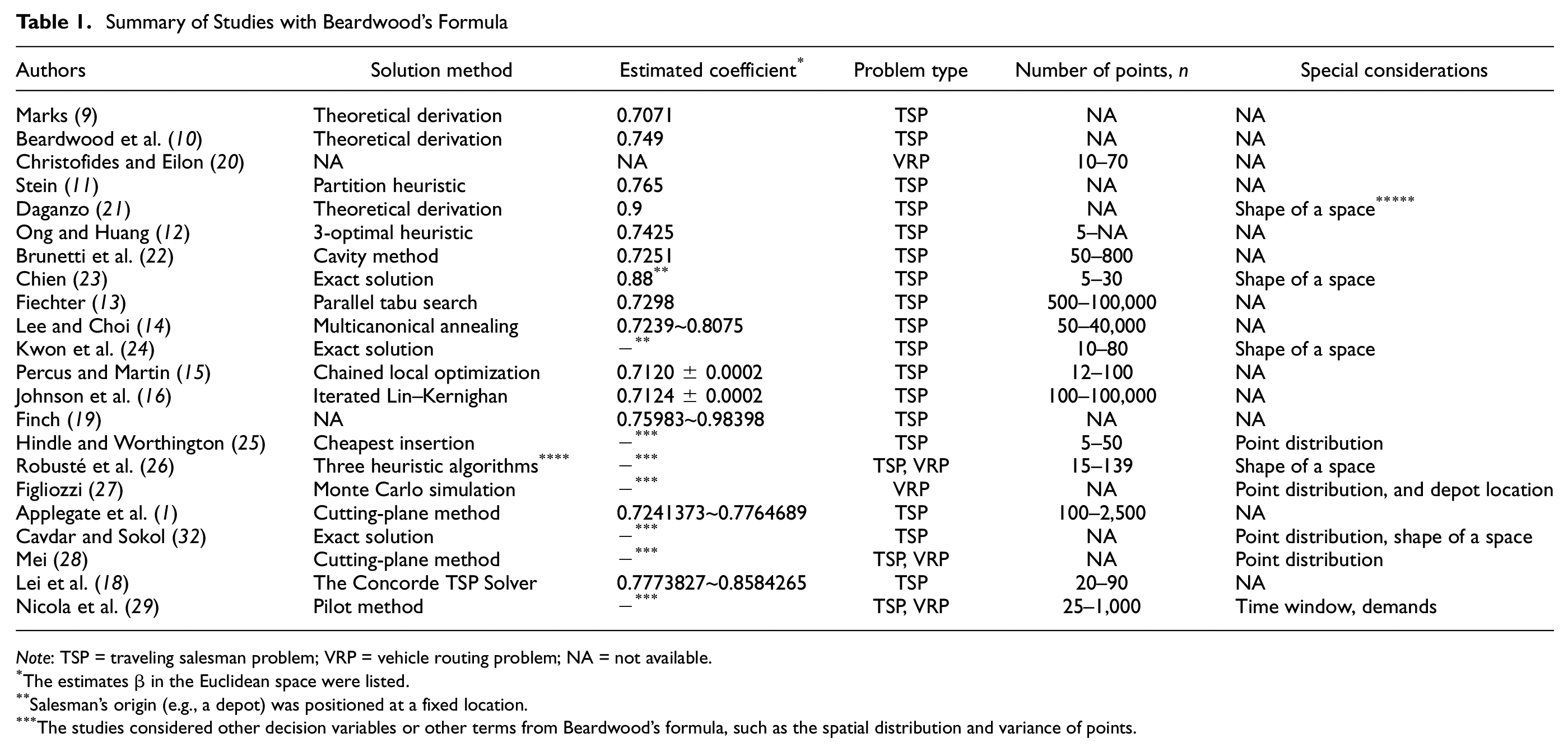
Note: TSP = traveling salesman problem; VRP = vehicle routing problem; NA = not available.

The estimates β in the Euclidean space were listed.

Salesman’s origin (e.g., a depot) was positioned at a fixed location.

***

The studies considered other decision variables or other terms from Beardwood’s formula, such as the spatial distribution and variance of points.

Although most of the coefficients cluster around 0.7, a few studies showed outlying values exceeding 0.8 for the following reasons:

Experimental settings (e.g., coefficients derived from worst-case TSP tour lengths [19]) and

Shapes of area (e.g., elongated [21] and sectorial-shaped area [23]).

This is further explained below.

Approximations for TSP Variants and Vehicle Routing Problem Tour Lengths

For the TSP variants and vehicle routing problem (VRP), several researchers have attempted to estimate the coefficient, β, through both analytical and experimental studies for different operational settings, such as considered vehicle capacity, zone shape, geometry, or point distributions. The major difference between the TSP and VRP is whether the problem considers vehicle loading capacities, time constraints, or time windows ( 30 ). The TSP solution would have a single route served by one vehicle, whereas the VRP has multiple routes possibly served by multiple vehicles. As such, the number of vehicles should be known a priori for VRP problems. Alternatively, a single TSP route can be split into several equal tours with an optimistic assumption that a penalty in relation to extra travel distance does not exist ( 31 ).

Christofides and Eilon first incorporated a vehicle capacity per tour in the formula and suggested approximations to the VRP tour length based on the shape and area of a region ( 20 ). Daganzo proposed an intuitive approximation for a generic irregular service zone, which was divided into multiple subareas containing clusters of points ( 21 ). A vehicle route was developed to serve each cluster. In this setting, he estimated β at 0.9 for Euclidean- and 1.15 for rectilinear space. Although β for the Euclidean space might overpredict the tour distance, it suites spaces with typical shapes.

Chien derived the constant β at 0.88 through empirical simulations and multiple regressions ( 23 ). The paper considered 16 different shapes varying in the (1) elongation and (2) angle of space. Rectangular areas with different length-to-width ratios from 1 to 8 were proposed in Figure 2a. Sectorial-shaped areas were developed with eight central angles from 45° to 360°, as illustrated in Figure 2b. The starting point (i.e., a depot) was positioned at the lower left side of the service area. From generated TSP instances, the best-fitted coefficients for Beardwood’s formula were derived through OLS regression.

Figure 2.

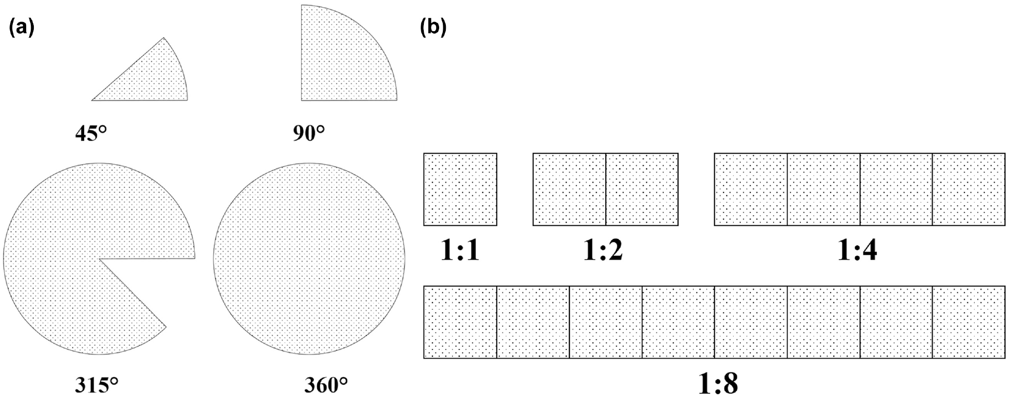
Shape of areas developed by Chien ( 23 ): (a) elongation for rectangular areas and (b) angle of sectorial-shaped areas.

Aside from the widely used form of Beardwood, later studies included various terms in the models, such as a length-to-width ratio or area of the smallest rectangle that covered all points. Kwon et al. ( 23 ) carried out both simulations and OLS regressions to test the previous variations (i.e., Beardwood et al. [10], Daganzo [21], and Chien [23]). To the best of our knowledge, most tour length approximations are based on regression methods since an increase in the TSP tour lengths associated with n values is nonlinear and can be effectively fitted with the square root form to obtain a reasonably good R². However, another approach was attempted by Chien ( 23 ). That research team also compared results from the regression with a neural network (NN) model for estimating the TSP tour length; the latter model provided slightly better approximations than the former. It is noted that the NN model was difficult to interpret geometrically owing to its characteristic as a so-called black box. Alternative expressions for estimating TSP tour lengths were developed by Hindle and Worthington, as presented in Equation 2 ( 25 ),

Average TSP distance = a \times n + b \times \ln (n) + c

(2)

where a, b, and c are constants in a 100 × 100 unit square: a = 3.63, b = 85.78, and c = 62.67. Two models were proposed based on demand patterns, namely uniformly random and probabilistic point distribution. The probabilistic demands were designed to simulate point distributions and settlement patterns.

Anther expression for the approximation is considered by Cavdar and Sokol, as presented in Equation 3 ( 32 ),

\begin{matrix} L ≅ 2.791 \sqrt{n (cstde v_{x} \cdot cstde v_{y})} \\ + 0.2669 \sqrt{nA (stde v_{x} \cdot stde v_{y}) / (\bar{c_{x}} \cdot \bar{c_{y}})} \end{matrix}

(3)

where

cstdev_x and cstdev_y are the standard deviations of x (horizontal) and y (vertical) coordinates from center point,

stdev_x and stdev_y are the standard deviations of the x and y coordinates,

$\bar{c_{x}}$ and $\bar{c_{y}}$ are the average distances of points to the central x and y coordinate, and

A is a zone size.

By incorporating the dispersion of points from the center, the approximation can estimate average TSP tour length without having the exact point distribution. However, compared with Beardwood’s variants (i.e., $β \sqrt{nA}$ ), the use of the model can be complicated for the computation of variables. In addition, the authors report that the estimated TSP tour lengths are underestimated if n < 1,000.

Special Considerations in Tour Length Approximations

Later studies for TSP approximations considered zone shape, geometry, or point distributions. An extended version of Daganzo’s approximation ( 21 ) that considered circular and elliptical spaces was proposed by Robusté et al. ( 26 ). Figliozzi proposed VRP tour length approximations using six different spatial distributions ( 27 ). His models also considered time windows, demands, and depot location. The study showed that time windows negatively affected the accuracy of the models; the time windows increased travel distance not only because the number of routes was increased but also because the distance between points per route was increased. Cavdar and Sokol developed approximations, where the point distribution was not uniform and random ( 32 ). The approximation models consisted of a few variables (e.g., the standard deviations of coordinates and of distances between the point and center in a region). The models were tested with different spatial distributions, including uniform and triangular distribution. In addition, the models also performed well for various shapes of a space, such as a triangular or polygonal service zone. Mei incorporated spatial distributions in approximating the tour lengths ( 28 ). The average nearest neighbor index was introduced for measuring the dispersion of points; the index utilized the distance between the centroid and each point. As the point distribution changed from dense (e.g., clustered) to dispersed, the estimates for β increased linearly. Nicola et al. proposed approximations based on regression models by adding more variables, such as time windows, vehicle capacities, and demands ( 29 ). The proposed model was compared with the previous models from Cavdar and Sokol ( 32 ) and Hindle and Worthington ( 25 ).

Guidelines for Using Tour Length Approximations

Larson and Odoni pointed out that all these expressions could provide a good approximation if (1) one of the measurements (e.g., width) of space was not much greater than the other measurement (e.g., length) of a region, and (2) no obstructions or boundaries existed in the region ( 31 ). Such conditions for a tour’s operating zone were generally called “fairly compact and fairly convex.” For rigorous definitions of this rule of thumb, numerous measures for both compactness and convexity had been proposed in the literature. Compactness measures were borrowed from geometric concepts, such as perimeters, areas, centroids, and vertices ( 33 ). Some measures are as follows: (1) length–width ratio: the ratio between the length and width of the minimum bounding rectangle; (2) convex hull: the ratio of the area between space and minimum bounding convex hull (i.e., the smallest convex polygon containing all the given points); and (3) Polsby–Popper: the ratio of the area of the space to the squared perimeter of the space. Similarly, convexity measures have been based on the area or boundary of space ( 34 ). A boundary-based convexity measure is computed as the ratio of the perimeter of space and that of convex hull. An area-based convexity measure computes the normalized average visible area of space, divided by the area of the space ( 35 , 36 ). The latter method is slightly more challenging to compute.

Most approximation errors here tend to approach zero as n increases, that is, asymptotically approaching a certain number. The convergence for TSP tour length approximations can be observed between n = 20 and n = 316,228 ( 1 , 16 , 18 ). The estimated coefficients, β, only decrease with increases in n values. Therefore, when using the approximations for small n, the users must account for discrepancies (e.g., lower/upper confidence intervals [15, 16], treatments for violating approximation assumptions, or adjustment factors reflecting point distribution).

Experimental Approach

Experimental Procedures: Point Generations, Heuristics, and Sample Size

Except for the theoretical derivations of Beardwood’s coefficients in Table 1, this section shed light on the derivation of the estimates, β, from experiments. The experimental method is illustrated in Figure 3. First, n points are generated according to a given distribution in a unit space whose area is one. For the point generation, most studies focus on a random and uniform distribution, while the shape of space is limited to a unit square. Random numbers provided in recent simulation programs are generated with the congruential algorithm, which has been widely used in programming to mimic randomness ( 36 ). By generating two random numbers uniformly distributed in the interval (0, 1), the numbers are regarded as an x- and y coordinate of a point in the space; each point in the x–y plane with both x and y between 0 and 1 is equally likely to be selected. Second, a solution method is chosen to compute optimized TSP tour lengths. For every TSP run, the visited points are regenerated after the TSP solution is obtained. From Table 1, no clear preference or explanation is apparent from researchers in choosing the solution method. Furthermore, no consensus exists on the “best” heuristic algorithm for solving the TSP instances, as shown in Table 2; ranks imply the shortest TSP solution, whereas percentage differences show the ratio between the best solution and the solution obtained by the selected heuristic method. For instance, a simulated annealing (SA) algorithm performed better than a genetic algorithm (GA) about 1.7% in accuracy from Adewole et al. comparison ( 38 ). This is done mainly because the results sensitively vary with some parameter values of heuristic methods and computation time.

Table 2.

Comparison of Heuristic Algorithms

n	Authors	Category	Solution method														Note
			SA	TS	GA	MA	BCO	ACO	FA	CS	HC	PSO	NN	GH	HS	LK
10	Adewole et al. ( 38 )	Rank	1	NA	2	NA
10	Adewole et al. ( 38 )	Difference, %	0.0	NA	1.7	NA
10	Gupta ( 39 )	Rank	1	2	7	6	8	3	3	3	NA
10	Gupta ( 39 )	Difference, %	0.0	0.0	−5.6	−5.7	−5.2	−5.7	−5.7	−5.7	NA
10	Damghanjiza and Mazidi ( 40 )	Rank	5	NA	1	NA		2	NA		4	3	NA				Not a random point generation
10	Damghanjiza and Mazidi ( 40 )	Difference, %	NA	NA	NA	NA		NA	NA		NA	NA	NA				Not a random point generation
15	Adewole et al. ( 38 )	Rank	1	NA	2	NA
15	Adewole et al. ( 38 )	Difference, %	0.0	NA	24.9	NA
15	Ansari et al. ( 2 )	Rank	1	NA				2	NA
15	Ansari et al. ( 2 )	Difference, %	0.0	NA				5.7	NA
16	Gupta ( 39 )	Rank	7	8	3	6	5	4	2	1	NA
16	Gupta ( 39 )	Difference, %	−19.4	−19.4	−2.2	−7.3	−4.4	−2.2	−2.2	0.0	NA
20	Adewole et al. ( 38 )	Rank	1	NA	2	NA
20	Adewole et al. ( 38 )	Difference, %	0.0	NA	50.2	NA
20	Abdulkarim and Alshammari ( 41 )	Rank	NA		1	NA							2	3	NA		Elongated space
20	Abdulkarim and Alshammari ( 41 )	Difference, %	NA		0.0	NA							32.8	8.4	NA		Elongated space
20	Ansari et al. ( 2 )	Rank	1	NA				2	NA
20	Ansari et al. ( 2 )	Difference, %	0.0	NA				39.0	NA
25	Adewole et al. ( 38 )	Rank	1	NA	2	NA
25	Adewole et al. ( 38 )	Difference, %	0.0	NA	4.4	NA
25	Ansari et al. ( 2 )	Rank	1	NA				2	NA
25	Ansari et al. ( 2 )	Difference, %	0.0	NA				11.9	NA
25	Gupta et al. ( 42 )	Rank	NA			3	NA		1	NA					2	NA
25	Gupta et al. ( 42 )	Difference, %	NA			18.5	NA		0.0	NA					11.2	NA
29	Gupta ( 39 )	Rank	6	8	3	4	7	5	2	1	NA
29	Gupta ( 39 )	Difference, %	111.6	159.4	0.1	0.4	128.4	10.3	0.1	0.0	NA
30	Gupta ( 39 )	Rank	3	5	3	7	6	8	2	1	NA
30	Gupta ( 39 )	Difference, %	0.5	0.8	0.5	3.8	2.3	7.4	0.5	0.0	NA
30	Ansari et al. ( 2 )	Rank	1	NA				2	NA
30	Ansari et al. ( 2 )	Difference, %	0.0	NA				25.4	NA
40	Adewole et al. ( 38 )	Rank	1	NA	2	NA
40	Adewole et al. ( 38 )	Difference, %	0.0	NA	3.3	NA
42	Ansari et al. ( 2 )	Rank	1	NA				2	NA
42	Ansari et al. ( 2 )	Difference, %	0.0	NA				20.3	NA
50	Adewole et al. ( 38 )	Rank	1	NA	2	NA
50	Adewole et al. ( 38 )	Difference, %	0.0	NA	32.9	NA
50	Ansari et al. ( 2 )	Rank	1	NA				2	NA
50	Ansari et al. ( 2 )	Difference, %	0.0	NA				23.4	NA
50	Gupta et al. ( 42 )	Rank	NA			3	NA		1	NA					2	NA
50	Gupta et al. ( 42 )	Difference, %	NA			35.0	NA		0.0	NA					21.6	NA
51	Gupta ( 39 )	Rank	7	8	4	6	5	2	3	1	NA
51	Gupta ( 39 )	Difference, %	197.6	215.5	4.0	6.9	4.5	0.0	1.6	0.0	NA
59	Damghanjiza ( 40 )	Rank	5	NA	1	NA		2	NA		4	3	NA
59	Damghanjiza ( 40 )	% Difference	NA	NA	NA	NA		NA	NA		NA	NA	NA
60	Adewole et al. ( 38 )	Rank	1	NA	2	NA
60	Adewole et al. ( 38 )	Difference, %	0.0	NA	24.0	NA
75	Gupta et al. ( 42 )	Rank	NA			3	NA		1	NA					2	NA
75	Gupta et al. ( 42 )	Difference, %	NA			50.4	NA		0.0	NA					39.2	NA
100	Abdulkarim and Alshammari ( 41 )	Rank	NA		2	NA							3	1	NA
100	Abdulkarim and Alshammari ( 41 )	Difference, %	NA		9.3	NA							14.4	0.0	NA
100	Gupta et al. ( 42 )	Rank	NA			3	NA		1	NA					2	NA
100	Gupta et al. ( 42 )	Difference, %	NA			45.7	NA		0.0	NA					36.8	NA
100	Crisan et al. ( 43 )	Rank	NA					1	NA							1
100	Crisan et al. ( 43 )	Difference, %	NA					0.0	NA							0.0

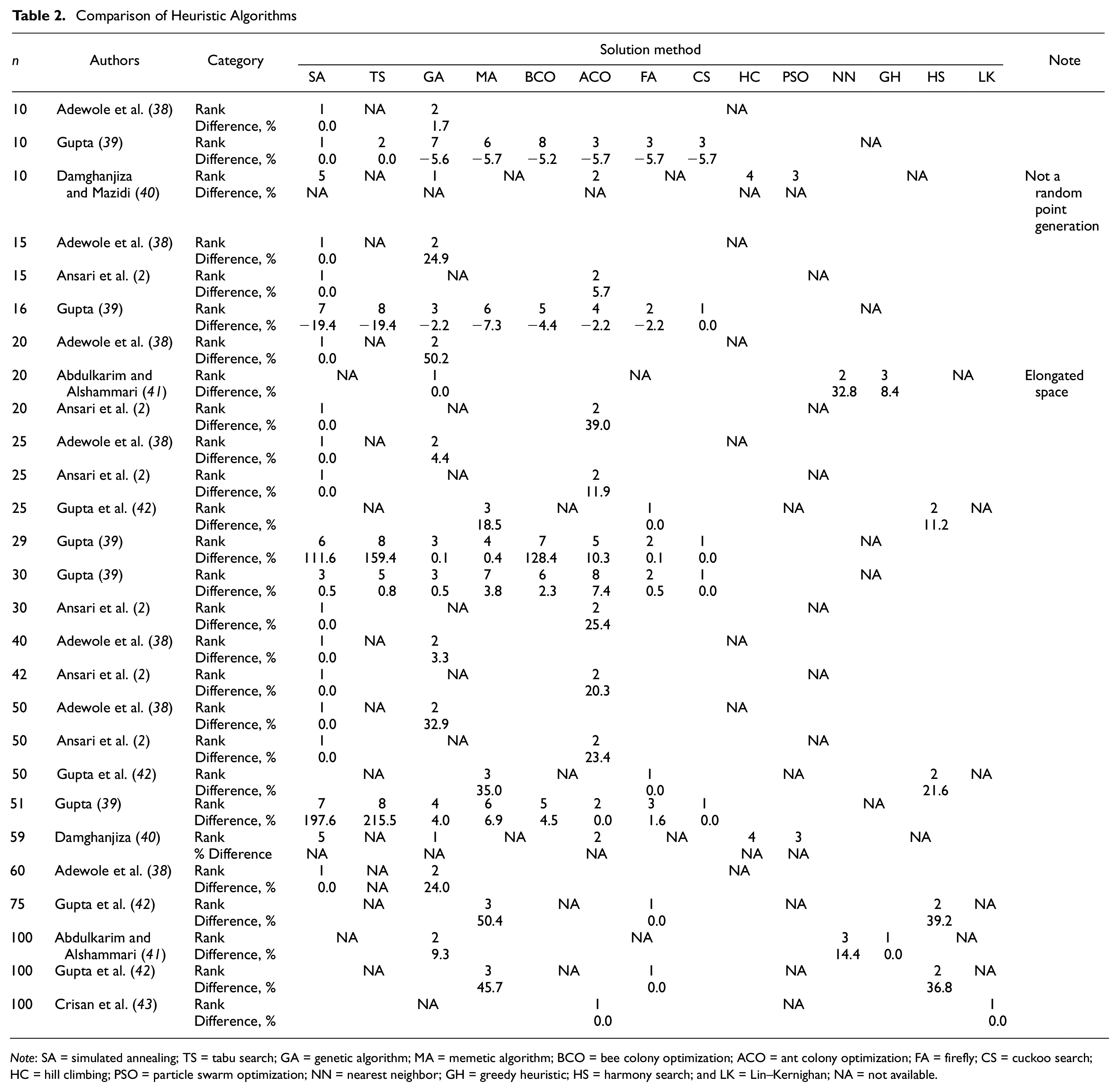
Note: SA = simulated annealing; TS = tabu search; GA = genetic algorithm; MA = memetic algorithm; BCO = bee colony optimization; ACO = ant colony optimization; FA = firefly; CS = cuckoo search; HC = hill climbing; PSO = particle swarm optimization; NN = nearest neighbor; GH = greedy heuristic; HS = harmony search; and LK = Lin–Kernighan; NA = not available.

Figure 3.

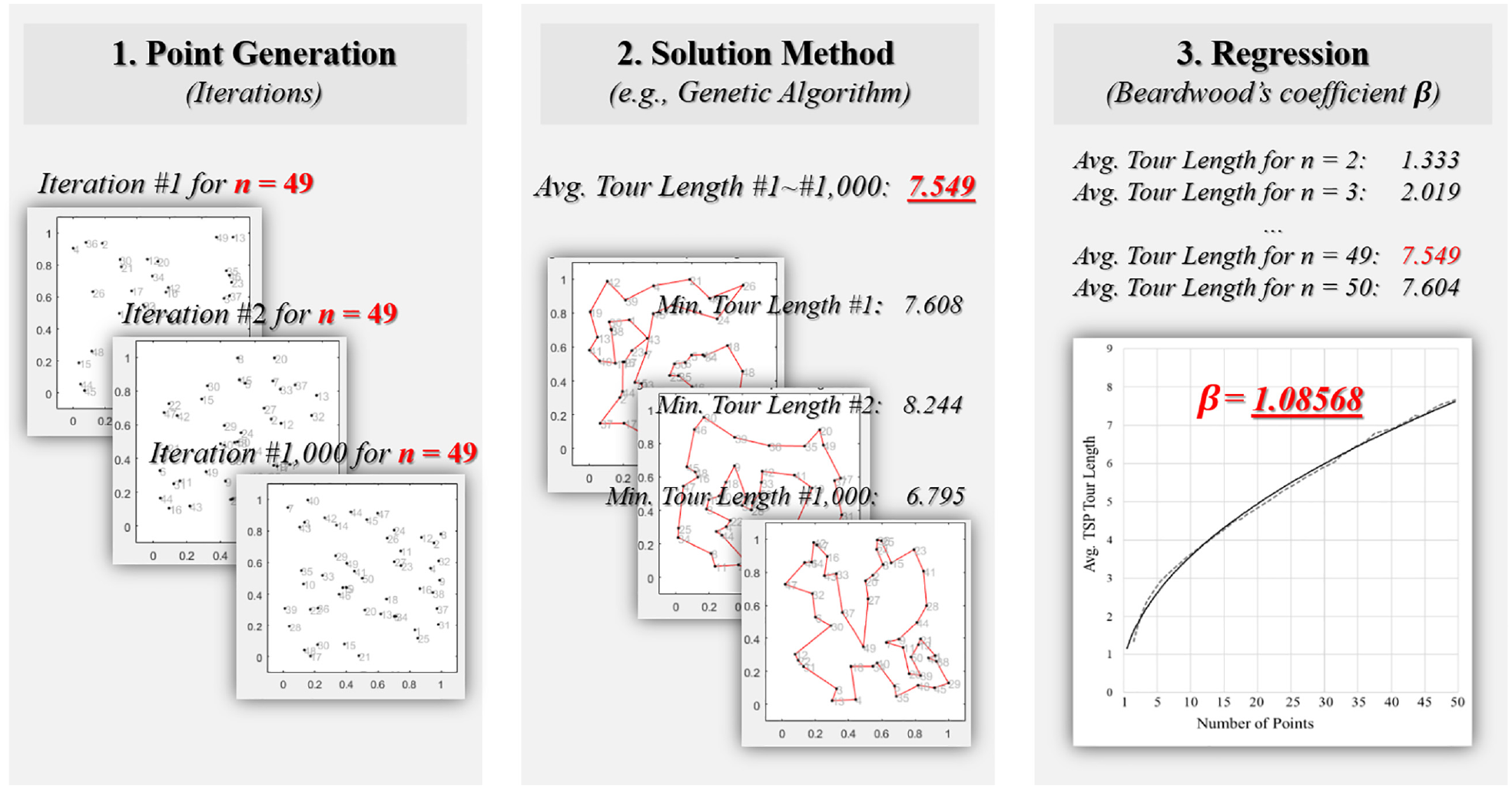
Overall process for estimating Beardwood’s coefficient β.

In Adewole et al., an SA procedure for the optimized TSP tour lengths ranging from an n of 10 to 60 performed better than a GA ( 38 ). The GA provided a good solution if the time was sufficient, meaning that a large population size was provided. In contrast, Damghanijazi and Mazidi showed that the GA performed best in searching for the TSP solution for 10- and 59-points; the SA and hill climbing methods were the worst ( 40 ). More comparisons for the performance of heuristics have been conducted by Gupta ( 39 ), Ansari et al. ( 2 ), Abdulkarim and Alshammari ( 41 ), and Gupta et al. ( 42 ). Crisan et al. examined the quality of the TSP solutions based on a structure of a TSP instance; the instances were classified as semistructured, and unstructured (randomly uniform) ( 43 ). The study then used a population-based ant colony optimization and a local search Lin–Kernighan heuristic for n ranging from 100 to 2,900. At n = 100, both heuristics provided the same optimized tour length. For a study conducted by Antosiewicz et al., six well-known metaheuristic algorithms were compared for n values ranging from 20 to 80 ( 44 ). The key idea was to find the best solution method when the computation time was restricted (e.g., 100 s). The authors presented several criteria for performance (e.g., accuracy, computation time, and standard deviation); however, none of the algorithms outperformed the others for all the suggested criteria. Third, repeated iterations on a given n are produced. After the predefined iterations for each n are reached (e.g., 1,000 runs per n values), the TSP tour lengths for each n values are averaged. Then, the repeated runs move next for n + 1. Finally, the averaged TSP tour length is fitted with OLS regression.

In brief, this study summarized and compared 14 metaheuristics from the literature as TSP solvers. However, researchers reached no consensus on choosing the best performing algorithm/heuristic for TSP instances. Instead, each algorithm has unique features and parameters that may be preferred for a particular research purpose.

The recommended sample size (i.e., the number of intervals in the 3rd column of Table 3) for running a regression should exceed 23, according to Green ( 45 ). Green compiled a comprehensive guide for choosing the minimum sample size as a function of the number of independent variables and effect size (e.g., a correlation between two variables); the effect size referred to standardized measures of the size of the mean difference, which generally used in multiple regression analysis. Several metrics could be used for deriving the effect size, such as Cohen’s d (t distribution) or ω (χ² distribution). If the effect size was small, many observations was needed. Sample sizes ranged from 23 (large effect size), to 53 (medium effect size), and 400 (small effect size). Alternatively, the number of iterations, N_i, is simply derived from Equation 4, where N_x is the number of estimates,

N_{i} \geq 50 + 8 \cdot N_{x}

(4)

Table 3.

Summary of Studies with Experiments for TSP/VRP Tour Approximation

Authors	Number of points, n	Number of intervals	Increment for n	Iterations per n^*	Shape of space	Problem type
Ong and Huang ( 12 )	5–NA	NA	Irregular	25	Square	TSP
Brunitti et al. ( 22 )	50–800	5	2x^**	500–20,000	Square	TSP
Fiechter ( 13 )	500–100,000	8	Irregular	10–30	Square	TSP
Lee and Choi ( 14 )	50–40,000	14	Irregular	4–1,300	Square	TSP
Kwon et al. ( 23 )	10–80	8	10	10	Irregular	TSP
Percus and Martin ( 15 )	12–100	8	Irregular	5–20	Square	TSP
Johnson et al. ( 16 )	100–316,228	7	$\sqrt{10}$ x^**	2–2,098	Square	TSP
Hindle and Worthington ( 25 )	5–50	46	1	500	Square	TSP
Applegate et al. ( 1 )	100–2,500	13	Irregular	10,000	Square	TSP
Lei et al. ( 18 )	20–90	8	10	100	Square	TSP
Nicola et al. ( 29 )	25–1,000	NA	NA	130–400	Square	VRP

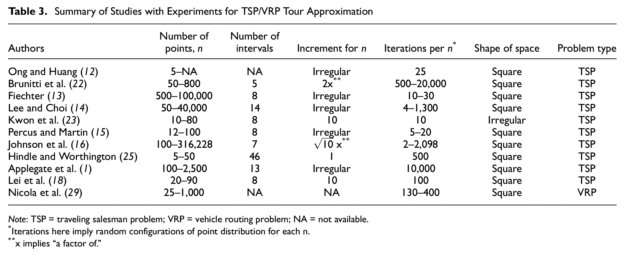
Note: TSP = traveling salesman problem; VRP = vehicle routing problem; NA = not available.

Iterations here imply random configurations of point distribution for each n.

x implies “a factor of.”

This guideline for estimating the instance size is simple and easy to use for a parsimonious model.

Literature with Experimental Approaches

Table 3 summarizes the experimental settings for tour length approximations from the literature. The number of points, n, in Table 3 is a range of n considered in estimating the coefficient, β. The number of intervals shows how many samples exist within that range (i.e., minimum point to maximum point), whereas the increment for n is a growth rate from min to max n. Note that irregular means n grows randomly in successive intervals.

Ong and Huang used 25 iterations for each n value starting from n = 5 ( 12 ). In their experiments, the sample variance of the optimized TSP tour length was shown to fluctuate, as shown in Figure 4. Although the variance was not discussed in detail for that study, Yang et al. presented the standard deviations of TSPs to model the travel time reliability (i.e., of tour lengths) ( 46 ).

Figure 4.

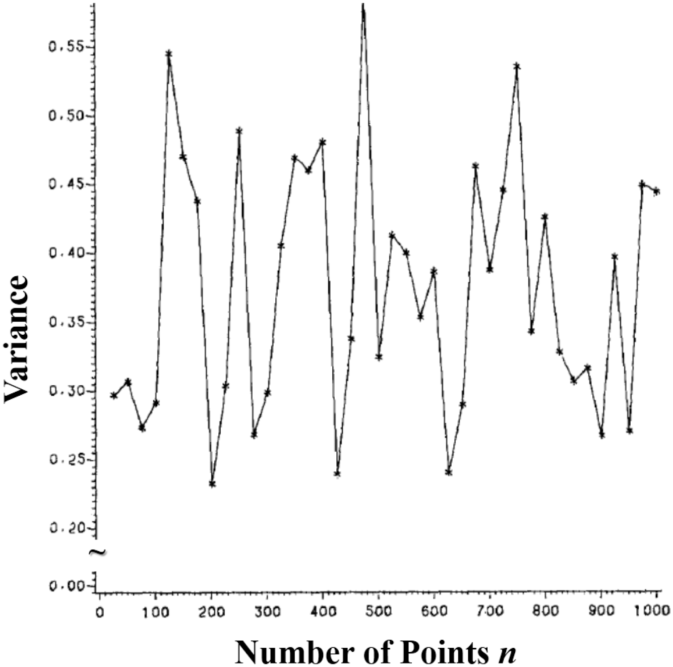
Sample variance of optimized traveling salesman problem (TSP) tour lengths by Ong and Huang ( 12 ).

Brunetti et al. found TSP solutions for their selected n values, which were 50, 100, 200, 400, and 800 ( 22 ). For each n, iterations ranged from 500 to 20,000. Lee and Choi conducted different iterations for the selected 14 intervals of n values, where the values ranged from 50 to 40,000 ( 14 ). As few as four iterations were used for large n values (i.e., n = 40,000), whereas 1,300 iterations were conducted for small n values (i.e., n = 50).

Using the eight intervals of n, Fiechter ran 10 to 30 iterations for each n ( 13 ). As Kwon et al. separated training and testing sets for the optimized TSP tour lengths, the number of instances was smaller than in other studies ( 23 ). For Johnson et al., n ranged from 100 to 316,228 points, increasing by factors of $\sqrt{10}$ ( 16 ). The exact TSP tour lengths were obtained for n values between 100 and 316. Then, the number of iterations decreased as n increased. Percus and Martin derived the TSP instances for the eight n values between 12 and 100; iterations were conducted between five and 12 runs ( 15 ). Unlike other researchers, Hindle and Worthington conducted the iterations with n increments of one ( 25 ).

Applegate et al. ran 10,000 iterations for generating the TSP instances visiting each n values ( 1 ). In their experiments, an increment of 100 was chosen for n between 100 and 1,000. Beyond n = 1,000, the increment of 500 was selected between 1,500 and 2,500 for n values. In Lei et al. experiments were conducted with 100 iterations for each n ranging from 20 to 90 ( 18 ). The number of iterations for large n increased in Nicola et al. ( 29 ). As half of the TSP instances were used for test sets, the unused instances were excluded in Table 3. In brief, the number of iterations per n was arbitrary. Some researchers suggested descriptive statistics (e.g., mean or standard deviation) and normality test for the obtained TSP instances ( 3 , 11 , 13 ). From this, one can better understand the central tendency and variability of the generated TSP instances. In addition, the instances with few n values can be compared with those for large n values.

Summary

This study reviewed existing tour length approximations dating back to 1940. Before Beardwood et al. developed their common formula in the late 1950s, the existing studies focused on theoretical derivation of the TSP tour length approximation ( 10 ). As more advanced computers and efficient solution methods were introduced, researchers explored accurate coefficients for the formula. After Daganzo considered realistic aspects of tours ( 21 ), recent studies have focused on various conditions (e.g., shape of service area or spatial distribution). The following section discusses some remaining gaps in the literature.

Most reviewed studies focused on the derivation of asymptotic coefficients for the TSP tour length; the estimated coefficients were based on a relatively large number of points visited per tour, at least five or more visited points in the 5th column of Table 1 ( 12 , 23 ). However, without using the approximations estimated with appropriate n values, the approximated distances would be inaccurately estimated. First, this is attributed to a downward trend of the square root form $\sqrt{n}$ , As more optimized TSP instances from large n values are used for fitting a regression, smaller coefficients would be estimated. Second, a larger increment (observable in the 4th column of Table 3) results in a less accurate value of the coefficient, β, because of the missing samples. Additional (smaller) intervals improve estimates for nonlinear relations by reducing interpolation errors.

In experimental approaches for Beardwood’s coefficients, the number of iterations for obtaining the optimal TSP tour length significantly varied in the existing studies, as shown in the 5th column of Table 3. Kwon et al. ( 23 ), Applegate et al. ( 1 ), and Lei et al. ( 18 ) used the same runs across all n values, whereas others did not present any criteria for the number of iterations (e.g., fewer iterations for large n values, and vice versa). Therefore, consistent runs would help in providing descriptive statistics of each n (e.g., mean, median, standard deviation, skewness, or kurtosis); the dataset of the optimum tour lengths can be investigated further, such as by using sample variance provided in Ong and Huang in Figure 4 ( 12 ). If the computation cost is affordable, large runs (e.g., 1,000 iterations per n value) would provide more reliable estimates of β.

In addition, the estimates for β change not only with the value of n but also with other factors (e.g., the point distribution or shape of space). Approximations considering many variables (e.g., distribution-free approximations) may be less flexible than Beardwood’s formula because of the required variables that are often unavailable or known a priori, such as the number of vehicles, length-to-width ratio, predetermined number of routes, or standard deviations of a point distribution in space. Adding more variables may increase the accuracy of the approximations as well as their complexity. If approximations become too complicated, solving the exact solution may be preferable. Therefore, researchers should consider such tradeoffs for approximations.

For approximating a TSP tour length with few points, users can apply the results from Kwon et al. ( 23 ), Percus and Martin ( 15 ), and Hindle and Worthington ( 25 ). As summarized in Table 3, the recommended approximations are derived from small n values with a reasonable number of intervals. Readers should understand whether the tour lengths for the visited points can be appropriately approximated; zone shape and distribution of points should be consistent with those used in the previous studies to derive such approximations.

In brief, the approximations estimating average tour lengths for relatively small n values are needed for analyzing and planning transportation systems whose vehicles have limited carrying capacities. The review conducted for this study found that several factors affect the value of the coefficient, β. It would worth investigating to what extent each factor changes β and possibly integrate all factors within a single equation. The new approximations may consider some potential extensions beyond the existing literature, as suggested below.

Distance metrics: at least two types of distance measures can be considered, namely Euclidean and rectilinear. In Euclidean space, movement directions are unrestricted and, therefore, the shortest air distances apply. In rectilinear space where movements are restricted to two orthogonal coordinates, as in rectangular grid street networks, travel distances are longer. For irregular networks distances can be approximated by multiplying Euclidean distances with appropriately computed circuity factors.

Shape of service area: although an exact shape of service area varies with roadway geometry, the basic shape categories to be considered are square and circular. The elongations of service areas can be further investigated with changes in their length-to-width ratios.

Distribution of points: the effects of concentrations of points, n, toward a particular direction (e.g., nonuniform distribution of the points) or in certain clustering patterns may be explored.

Approximations for tour distances with time windows or constraints on the sequence of visits.

Approximations for tours by vehicles with limited capacity, which may constrain the sequence of pickups and dropoffs.

Investigations of solution accuracy or discrepancies between approximations and exact solutions.

Footnotes

Author Contributions

The authors confirm contributions to the paper as follows: study conception and design: Y. Choi, P. Schonfeld; data collection: Y. Choi; analysis and interpretation of results: Y. Choi, P. Schonfeld; draft manuscript preparation; Y. Choi, P. Schonfeld. All authors reviewed the results and approved the final version of the manuscript.

Declaration of Conflicting Interests

The authors declared no potential conflicts of interest with respect to the research, authorship, and/or publication of this article.

Funding

The authors received no financial support for the research, authorship, and/or publication of this article.

ORCID iDs

Youngmin Choi

Paul M. Schonfeld

References

Applegate

Bixby

Chvatal

Cook

The Traveling Salesman Problem: A Computational Study. Princeton University Press, Princeton, 2006.

Ansari

Basdere

Ouyang

Smilowitz

Advancements in Continuous Approximation Models for Logistics and Transportation Systems: 1996–2016. Transportation Research Part B: Methodological, Vol. 107, 2018, pp. 229–252. https://doi.org/10.1016/j.trb.2017.09.019

Korte

Vygen

Combinatorial Optimization: Theory and Algorithms. 2008. https://doi.org/10.1007/978-3-540-71844-4_21. Accessed July 26, 2020.

Chang

S. K.

Schonfeld

Optimization Models for Comparing Conventional and Subscription Bus Feeder Services. Transportation Science, Vol. 25. No. 4, 1991, pp. 281–298. https://doi.org/10.1287/trsc.25.4.281.

Kim

Schonfeld

Integration of Conventional and Flexible Bus Services with Timed Transfers. Transportation Research Part B: Methodological, Vol. 68, 2014, pp. 76–97. https://doi.org/10.1016/j.trb.2014.05.017.

Choi

Schonfeld

Lee

Shin

Innovative Methods for Delivering Fresh Food to Underserved Populations. Journal of Transportation Engineering, Part A: Systems, Vol. 147, No. 1, 2021, p. 04020140. https://doi.org.10.1061/JTEPBS.0000464.

Holguín-Veras

Patil

G. R.

Observed Trip Chain Behavior of Commercial Vehicles. Transportation Research Record: Journal of the Transportation Research Board, 2005. 1906: 74–80.

Mahalanobis

A Sample Survey of the Acreage under Jute in Bengal. The Indian Journal of Statistics, Vol. 4, No. 4, 1940, pp. 511–530. https://www-jstor-org-443.web.bisu.edu.cn/stable/40383954.

Marks

A Lower Bound for the Expected Travel Among m Random Points. The Annals of Mathematical Statistics, Vol. 19, No. 3, 1948, pp. 419–422. https://www-jstor-org-443.web.bisu.edu.cn/stable/2235651.

10.

Beardwood

Halton

Hammersley

The Shortest Path through Many Points. Mathematical Proceedings of the Cambridge Philosophical Society, Vol. 55, No. 4, 1959, pp. 299–327.

11.

Stein

D. M.

An Asymptotic Probabilistic Analysis of a Routing Problem. Mathematics of Operations Research, Vol 3. No. 2. 1978, pp. 89–101. https://www-jstor-org-443.web.bisu.edu.cn/stable/3689335.

12.

Ong

H. L.

Huang

H. C.

Asymptotic Expected Performance of Some TSP Heuristics: An Empirical Evaluation. European Journal of Operational Research, Vol. 43, 1989, pp. 231–238. https://doi.org/10.1016/0377-2217(89)90217-8.

13.

Fiechter

A Parallel Tabu Search Algorithm for Large Traveling Salesman Problems. Discrete Applied Mathematics, Vol. 51, 1994, pp. 243–267. https://doi.org/10.1016/0166-218X(92)00033-I.

14.

Lee

Choi

M. Y.

Optimization by Multicanonical Annealing and the Traveling-Salesman Problem. Computer Simulation Studies in Condensed-Matter Physics VII, Vol. 78, 1994, pp. 193–198.

15.

Percus

Martin

Finite Size and Dimensional Dependence in the Euclidean Traveling Salesman Problem. Physical Review Letter, Vol. 76, 1996, pp. 1188–1191. https://doi.org/10.1103/PhysRevLett.76.1188.

16.

Johnson

McGeoch

Rothberg

Asymptotic Experimental Analysis for the Held-Karp Traveling Salesman Bound. Proc., 7th Annual ACM-SIAM Symposium on Discrete Algorithms, Atlanta, GA, 1996, pp. 341–350.

17.

Franceschetti

Jabali

Laporte

Continuous Approximation Models in Freight Distribution Management. TOP, Vol. 25, 2017, pp. 413–433. https://doi.org/10.1007/s11750-017-0456-1.

18.

Lei

Laporte

Liu

Zhang

Dynamic Design of Sales Territories. Computers & Operations Research, Vol. 56, 2015, pp. 84–92. https://dx-doi-org.web.bisu.edu.cn/10.1016/j.cor.2014.11.008.

19.

Finch

Mathematical Constants. Cambridge University Press, Cambridge, 2003.

20.

Christofides

Eilon

Expected Distances in Distribution Problems. OR, Vol. 20, No. 4, 1969, pp. 437–443. http://doi.org/10.2307/3008762.

21.

Daganzo

The Length of Tour in Zones of Different Shapes. Transportation Research Part B: Methodology, Vol. 18B, No. 2, 1984, pp. 135–145. https://doi.org/10.1016/0191-2615(84)90027-4.

22.

Brunetti

Krauth

Mézard

Parisi

Extensive Numerical Simulations of Weighted Matchings: Total Length and Distribution of Links in the Optimal Solution. EPL (Europhysics Letters), Vol. 14, No. 4. 1991, p. 295. https://doi.org/10.1209/0295-5075/14/4/002.

23.

Chien

T. W.

Operational Estimators for the Length of a Traveling Salesman Tour. Computers & Operations Research, Vol. 19, No. 6, 1992, pp. 469–478. https://doi.org/10.1016/0305-0548(92)90002-M.

24.

Kwon

Golden

Wasil

Estimating the Length of the Optimal TSP Tour: An Empirical Study Using Regression and Neural Networks. Computers & Operations Research, Vol. 22, No. 10, 1995, pp. 1039–1046. https://doi.org/10.1016/0305-0548(94)00093-N.

25.

Hindle

Worthington

Models to Estimate Average Route Lengths in Different Geographical Environments. Journal of the Operational Research Society, Vol. 55, 2004, pp. 662–666. https://doi.org/10.1057/palgrave.jors.2601751.

26.

Robusté

Estrada

López-Pita

Formulas for Estimating Average Distance Traveled in Vehicle Routing Problems in Elliptic Zones. Transportation Research Record: Journal of the Transportation Research Board, 2004. 1873: 64–69.

27.

Figliozzi

Planning Approximations to the Average Length of Vehicle Routing Problems with Varying Customer Demands and Routing Constraints. Transportation Research Record: Journal of the Transportation Research Board, 2008. 2089: 1–8.

28.

Mei

Approximating the Length of Vehicle Routing Problem Solutions Using Complementary Spatial Information. George Mason University, 2005. http://mars.gmu.edu/handle/1920/9623 Accessed July 26, 2020.

29.

Nicola

Vetschera

Dragomir

Total Distance Approximations for Routing Solutions. Computers and Operations Research, Vol. 102. 2019, pp. 67–74. https://doi.org/10.1016/j.cor.2018.10.008.

30.

Kumar

Panneerselvam

A Survey on the Vehicle Routing Problem and its Variants. Intelligent Information Management, Vol. 4. No. 3. 2012, pp. 66–74. https://dx-doi-org.web.bisu.edu.cn/10.4236/iim.2012.43010.

31.

Larson

Odoni

Urban Operation Research. Dynamic Ideas, Prentice Hall, NJ, 1981.

32.

Cavdar

Sokol

A Distribution-Free TSP Tour Length Estimation Model for Random Graphs. European Journal of Operational Research, Vol. 243, No. 2, 2015, pp. 588–598. https://doi.org/10.1016/j.ejor.2014.12.020.

33.

Kaufman

King

Komisarchik

How to Measure Legislative District Compactness If You Only Know it When You See it. American Journal of Political Science, Vol. 65, No. 3, 2021, pp. 533–550.

34.

Zunic

Rosin

A New Convexity Measure for Polygons. IEEE Transactions on Pattern Analysis and Machine Intelligence, Vol. 26, No. 7, 2004, pp. 923–934.

35.

Stern

Polygonal Entropy: A Convexity Measure. Pattern Recognition Letters, Vol. 10, 1989, pp. 229–235. https://doi.org/10.1016/0167-8655(89)90093-7.

36.

Rote

, The Degree of Convexity. EuroCG 2013, Braunschweig, Germany, 2013.

37.

Moler

Numerical Computing with MATLAB. Society for Industrial and Applied Mathematics, 2008.

38.

Adewole

Otubamowo

Egunjobi

A Comparative Study of Simulated Annealing and Genetic Algorithm for Solving the Travelling Salesman Problem. International Journal of Applied Information Systems, Vol. 4. No. 4, 2012, pp. 6–12.

39.

Gupta

Solving TSP Using Various Meta-Heuristic Algorithms. International Journal of Recent Contributions from Engineering, Science & IT, Vol 1, No 2, 2013, pp. 22–26.

40.

Damghanijazi

Mazidi

Meta-Heuristic Approaches for Solving Travelling Salesman Problem. International Journal of Advanced Research in Computer Science, Vol. 8, No. 5, 2017, pp. 18–23.

41.

Abdulkarim

Alshammari

Comparison of Algorithms for Solving Traveling Salesman Problem. International Journal of Engineering and Advanced Technology, Vol. 4, No. 6, 2015, pp. 76–79.

42.

Gupta

Rana

Kansal

Comparison of Heuristic Techniques: A Case of TSP. Proc., 10th International Conference on Cloud Computing, Data Science & Engineering, Noida, India, 2020. https://doi.org/10.1109/Confluence47617.2020.9058211.

43.

Crisan

Nechita

Simian

On Randomness and Structure in Euclidean TSP Instances: A Study with Heuristic Methods. IEEE Access, Vol. 9. 2021, pp. 5312–5331. https://doi.org/10.1109/ACCESS.2020.3048774.

44.

Antosiewicz

Koloch

Kamiński

Choice of Best Possible Metaheuristic Algorithm for the Travelling Salesman Problem with Limited Computational Time: Quality, Uncertainty and Speed. Journal of Theoretical and Applied Computer Science, Vol. 7, No. 1, 2013, pp. 46–55.

45.

Green

How Many Subjects Does It Take To Do A Regression Analysis. Multivariate Behavioral Research, Vol. 26, 1991, pp. 499–510. https://doi.org/10.1207/s15327906mbr2603_7.

46.

Yang

Liang

Zhang

Liu

Abid

Statistical Modeling of Quartiles, Standard Deviation, and Buffer Time Index of Optimal Tour in Traveling Salesman Problem and Implications for Travel Time Reliability. Transportation Research Record: Journal of the Transportation Research Board, 2020. 2674: 339–347.