Bridge Response and Heavy Truck Classification Framework Based on a Two-Step Machine Learning Algorithm

Abstract

Collecting information on heavy trucks and monitoring the bridges which they regularly cross is important for many facets of infrastructure management. In this paper, a two-step algorithm is developed using bridge and truck data, by deploying sequentially unsupervised and supervised machine learning techniques. Longitudinal clustering of bridge data, concerning strain waveforms, is adopted to perform the first step of the algorithm, while image visual inspection and classification tree methods are applied to truck data concurrently in the second step. Both bridge and truck traffic must be monitored for a limited, yet significant, amount of time to calibrate the algorithm, which is then used to build a classification framework. The framework provides the same benefits of two data collection systems while only one needs to be operative. Depending on which monitoring system remains available, the framework enables the use of bridge data to identify the truck’s profile which generated it, or to estimate bridge response given the truck’s information. As a result, the present study aims to provide decision-makers with an effective way to monitor the whole bridge-traffic system, bridge managers to plan effective maintenance, and policymakers to develop ad hoc regulations.

Keywords

Infrastructure infrastructure management and system preservation bridge and structures management bridge data QC/QA policy and organization executive management issues data for decision-making data-driven decisions

With the rapid growth of highway transportation, monitoring the frequency of heavy loads on infrastructure elements, such as bridges, is of increasing importance. Many management decisions (pavement design and maintenance, enforcement, traffic monitoring, air quality models, inspection frequency, service life determination, and posting load limits) derive heavily from knowledge of the vehicles that typically traverse a bridge. Heavy trucks contribute significantly to pavement degradation, serviceability problems, and fatigue damage in structural elements ( 1 ). Studies have shown that the gross vehicle weight (GVW), axle weight, and axle configuration of heavy trucks all have bearing on the damage exhibited by a bridge’s deck, floor beams, girders, diaphragms, joints, and bearings ( 2 ). Having accurate knowledge of the type of heavy trucks, their frequency and the different responses of the bridge can be beneficial in planning effective maintenance interventions and promote overall safer use of the structure.

Collecting data concerning both the structure and its traffic is ideal, but not always economically sustainable, as it requires constant maintenance. However, it is not uncommon to collect either bridge data or traffic data, depending on the site’s criticalities. The goal of this paper is to propose an alternative to the long-term maintenance of two monitoring systems by making the best use of the bridge and traffic monitoring systems working simultaneously for only a limited amount of time, and to keep the benefits active even after one of the two systems is discontinued. To achieve this goal, a two-step algorithm and a classification framework are developed using both bridge and truck data. Given the challenges of handling large and different datasets (bridge and traffic data), powerful machine learning techniques are appropriately selected to develop the algorithm. Longitudinal clustering of bridge response is adopted to perform the first step of the algorithm, while image visual inspection and classification trees ( 25 ) are applied to traffic data concurrently in the second step. The outcome of the algorithm is successively used to build a classification framework for use when one of the two monitoring systems is discontinued. Given bridge response data, the framework provides information on the truck crossing the bridge or given truck information, it provides a potential bridge response.

The process is presented using a combination of traffic and bridge response data from a testbed bridge (proof of concept). Truck characteristics (gross vehicular weight, length, speed, weight of each axle, axle spacing) are collected from a weigh-in-motion (WIM) system, while strain waveforms are collected from a structural health monitoring (SHM) system installed on the bridge. Multiple use cases are also presented to show the applicability of the proposed framework and how it helps support bridge managers, owners, and policymakers in making more informed decisions concerning infrastructure and heavy traffic.

Technical Background

Traffic classification has always been an important area of research for infrastructure management. This study focuses on heavy traffic as they have a high chance to put infrastructure at a higher risk than lighter traffic ( 3 ). Despite the importance of monitoring heavy traffic patterns along bridges, existing traffic methods available in literature do not focus on important variations between heavy vehicles as they are not easily recognizable. This paper aims to fill this gap. Relevant studies of vehicle classification include Sun et al. ( 4 ), who developed an inductive classifying artificial network for vehicle classification. The classification is not done by the number of axles or spacing, but by “useful classes” such as passenger cars, sport utility vehicles, vans, buses, and trucks. Fiorillo and Goshn ( 1 ) developed a data-mining algorithm to analyze WIM data to identify and classify overweight trucks into permitted and illegal categories. They adopted a pattern recognition algorithm to cluster vehicles according to the Federal Highway Administration (FHWA) classification into four preliminary categories, then applied Bayesian conditional probability to identify illegal trucks. Battiato et al. ( 5 ) took a Bayesian approach to classify vehicles from videos into two classes, cars versus trucks. Mosa et al. ( 6 ) designed a model to classify vehicles into four categories (stopped car, moving car, stopped truck, and moving truck) using a soft radial basis cellular neural network (SRB-CNN) for the classification of inductive loop data. Simoncini et al. ( 7 ) used recurrent neural networks with long short-term memory to classify vehicles using GPS data acquired from each vehicle. They trained a model to predict three classes (light, medium, and heavy-duty).

Strain data have also been used for vehicle classification. Zhang et al. ( 8 ) presented a vehicle classification system based on measuring dynamic strain caused by vehicles crossing the pavement to obtain the corresponding vehicle characteristics. They tested and compared two support vector machine (SVM) classification algorithms to classify single sensor data and multiple sensor combination data. Yan et al. ( 9 ) developed a strain-based vehicle classification using neural networks, which was compared to a manual classification developed by the authors. The dataset consisted of strain records and videos from which they extracted class, weight, and speed of the vehicles by using principal component analysis (PCA). They considered all vehicles, from passenger cars to trucks. The results obtained with the neural network were compared with those obtained by using Bayesian inference. Shim et al. ( 10 ) applied three machine learning algorithms (naïve Bayesian, neural network, and SVM) to automatically classify vehicles into five classes, from small vehicles to trucks. The data were collected from strain gages installed on bridge-deck panels and PCA was used for feature extraction.

The use of longitudinal clustering in civil engineering is not as common as in other fields such as criminology ( 11 ), epidemiology ( 12 ), sociology ( 13 ), psychology, and psychiatry ( 13 – 15 ), where the use of functional data is more widespread. However, given the need to process unlabeled strain records and their longitudinal nature, this method resulted in a perfect fit to accomplish the task of step 1 of the algorithm presented in this work. On the other hand, for step 2 we use classification trees as this method allows predictions on the spot, and its output can be easily visualized and interpreted by a non-expert audience ( 16 ), which is in line with the goal of this paper to provide decision-makers with a user-friendly monitoring approach. Relevant studies that deployed clustering methods and classification tree are by Erman et al. ( 17 ), who used K-means and density-based spatial clustering of applications with noise to identify groups of traffic with similar characteristics and compared the results with the AutoClass algorithm. Jeng and Ritchie ( 18 ) combined decision tree and K-means clustering using inductive loop signature data to classify vehicles into FHWA categories. Another study which deployed, among other methods, decision trees is Hernandez et al. ( 19 ), who presented a multiple classifier system, which combines Naïve Bayes, decision trees, SVM, and neural networks to classify vehicles according to FHWA classifications using WIM and inductive loop data.

Methodology

The two-step algorithm shows how unsupervised and supervised machine learning methods can work together and interact to improve each other’s performance. The advantages of using machine learning approaches are listed in the following: (i) the structure of the problem is learned from the data as opposed to being predefined; (ii) machine learning is particularly strong at variable selection, unlike statistical approaches where variables are explicitly defined a priori; (iii) machine learning methods are known to have strong predictive power; and (iv) they work well with large datasets ( 20 ). Both bridge and traffic data are used in the calibration of the algorithm. Unsupervised learning is adopted in the first step, which consists of clustering bridge response concerning strain records. The goal of this step is to divide a set of bridge responses into subsets with similar characteristics using longitudinal K-means clustering developed by Genolini and Fallissard ( 21 ). Considering a set S of n objects, for each object an outcome variable Y at different time t is measured. y_il is the value of Y for the object i at time l, and the sequence y_i = (y_i1, y_i2, …, y_it) is the trajectory. The goal of clustering is to divide a set S into k homogeneous subsets by computing the distance between an object and the centroid of each cluster (this case uses the Euclidean distance) and assigning each object to the nearest cluster. Defining the optimal number of clusters can be challenging as it must be decided upfront. For this purpose, we use the Calinski–Haravbatz criterion ( 22 ) to select the optimal number of clusters (C), where (C) corresponds to the number of clusters k, which maximizes the between-matrix variance (B) and minimizes the within-matrix variance (W) (Equation 1).

C (k) = (\frac{trace (B)}{trace (W)}) \cdot (\frac{n - k}{k - 1})

(1)

High values of trace(B) indicate well-separated clusters, and low values of trace(B) indicate that the clusters are close to each other. In other words, high values of trace(W) indicate heterogeneous clusters, while low values of trace(W) indicate compact clusters, which is the ideal scenario. It is noteworthy that, although this criterion helps find the optimal number of clusters, it does not always find the correct solution, as discussed by Shim et al. ( 10 ). The clusters resulting from the analysis developed in the first step are then used in the second step as the classification tree’s categorical dependent variable.

Supervised learning is used in the second step to identify the profile of the truck (considering only FHWA class 9 and above) that generates each response of the bridge. This step is performed using two non-mutually exclusive methods—image visual inspection and classification tree—depending on data availability. The image visual inspection (or image processing, when the number of available photos to process is significantly large) qualitatively assigns a truck type (regular, logging truck, flatbed, etc.) using the photos taken by the WIM system. The classification tree ( 23 ) predicts the bridge response cluster that a truck can generate using the truck’s characteristics measured by the WIM system. The tree identifies which predictors, among all truck’s characteristics, are influencing the response. Classification trees are widely appreciated because of their interpretability and simplicity ( 24 ). The model structure can be summarized by the following equation (Equation 2):

g (x, θ) = \sum_{m = 1}^{M} c_{m} I (x \in R_{m})

(2)

At each split, the model divides the predictor’s space into rectangular regions where the predicted response $g (x, θ)$ is the average response c_m over the entire region R_m. M is the total number of regions or terminal nodes, and I is an indicator function equal to 1 or 0 depending on x belonging to R_m. N_m is the size of the mth terminal node (region) and θ represents all the parameters and the structure. The highest reduction of the sum of squared errors defines the best place to split the data set into regions. The model automatically identifies the most significant predictors by including them in the tree, repeating them multiple times, and placing them in higher positions of the tree. The prediction is revealed at the end of the final branch reached by following a known path. Deviance is used to calculate the goodness of fit ( 25 ).

Once the two-step algorithm (Figure 1) is calibrated, using both bridge and truck data, a classification framework is created. The framework shows which bridge response is associated with each truck. The main contribution of this framework is to provide the same benefits of having two monitoring systems while, in practice, only one is active. For each known strain response of the bridge, the framework can provide the profile of the heavy truck which generated it without having a traffic monitoring system. For each known truck, the framework can provide the bridge response associated with that specific truck with no need to directly monitoring the bridge (Figure 2).

Figure 1.

Flow chart of the two-step algorithm.

Figure 2.

Schematic description of the two-step algorithm and classification framework.

Proof of Concept

Bridge and Data

The Hurley bridge is the testbed structure used to develop and calibrate the two-step algorithm and the classification framework. It is a five-girder, three-span continuous steel bridge over two piers with a composite concrete deck and carries the two westbound lanes of US Highway 2 (US-2) over the Montreal River (the eastbound lanes cross on a separate but identical structure) between Ironwood, Michigan, and Hurley, Wisconsin. The overall length of the structure is 37 m (120 ft). The two lanes are 3.65 m (12 ft) wide and the two asymmetric shoulders are 3 m and 1.8 m (10 ft and 6 ft) (Figure 3). The structure is skewed by 30°. Concerns over possible effects of increased load limits on the US-2 corridor, including the subject bridge, led to an opportunity to measure both vehicle parameters and structural responses on a multi-year basis by installing a WIM system and an SHM. Logging is an important economic activity in the area, and load limits for logging trucks were increased in the subject corridor to promote transportation of timber from Michigan to a sawmill in Wisconsin approximately 64 km (40 miles) west of the subject bridge. Specifically, loaded logging vehicles exceeding Wisconsin GVW limitations are allowed to travel into Wisconsin along the US-2 corridor, provided the vehicles meet Michigan’s less stringent GVW regulations. For non-logging trucks, the GVW limit on the route is approximately 36.3 metric tons (80 kip); logging trucks are allowed to exceed this gross weight, and routinely do so. For these reasons, the Hurley bridge is an excellent testbed structure for this study.

Figure 3.

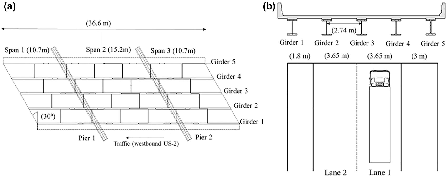
(a) Plan view and (b) cross section with truck position visualization.

WIM System

A commercial in-pavement WIM system, which allows measurements of moving vehicles without interrupting traffic, was installed approximately 60 m (200 ft) ahead of the bridge. The commercial system processes signals from the in-pavement sensors to determine vehicle properties such as GVW, overall length, axle weight and spacing, speed, lane of travel, and FHWA vehicle class. When the WIM system detects a truck classified as FHWA Class 9 or above, it signals the SHM system installed on the bridge.

SHM System

The Infrastructure Technology Institute at Northwestern University (NU-ITI) designed, constructed, and installed an autonomous long-term SHM system on the bridge ( 26 ). The sensors employed in this study are five strain gauges on the bottom flange of each of the five girders at mid-span, one of the high-stress regions on a girder. When the SHM system is triggered by the WIM system it starts recording dynamic strain waveforms (sampled at 100 Hz) every five seconds (Figure 4).

Figure 4.

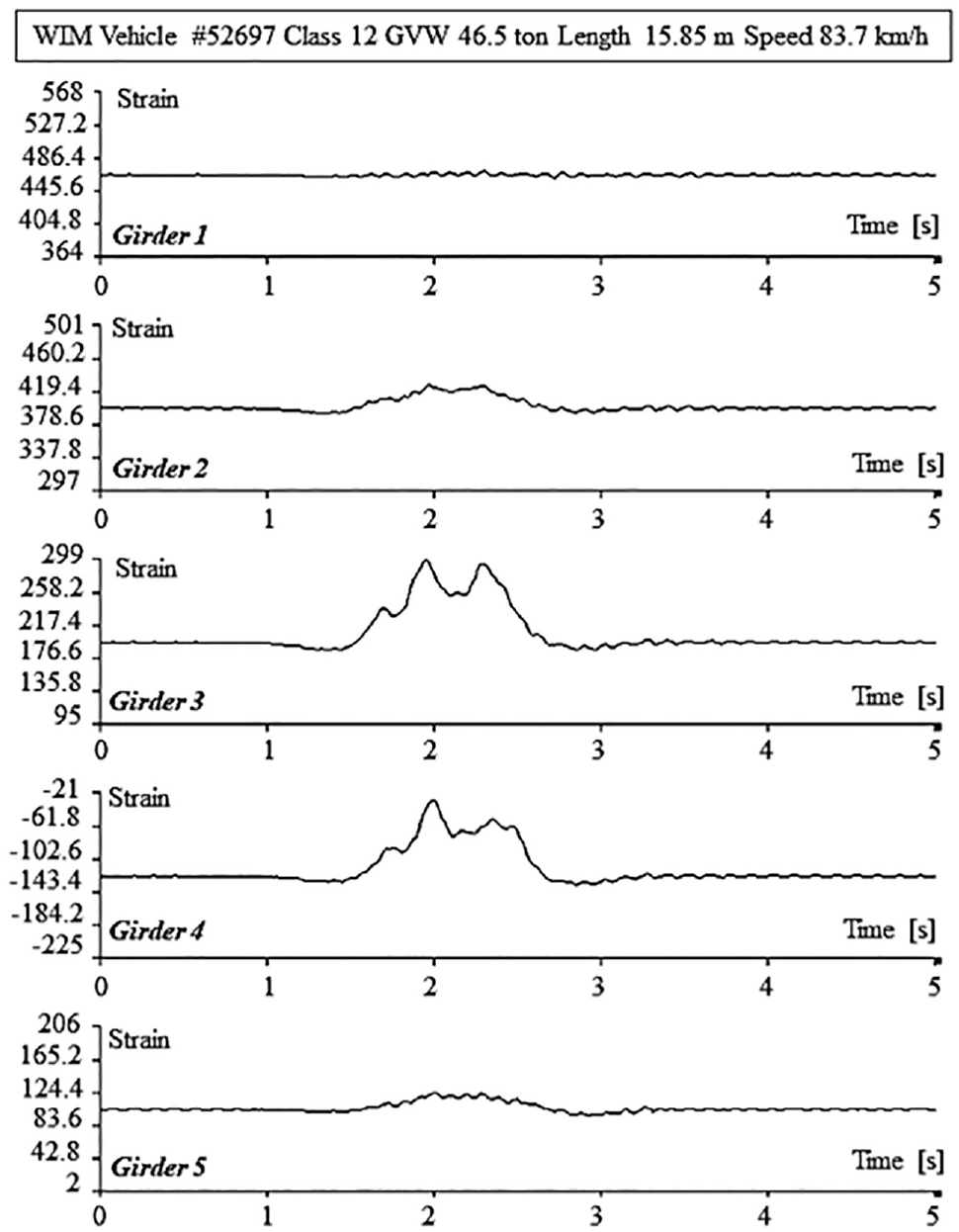
Dynamic response of five midspan strains caused by a truck in lane 1.

Data Pre-Processing

Data were continuously collected under live traffic for over three years (2010–2013), generating a unique long-term WIM–SHM combined dataset. To develop the two-step algorithm, both SHM and WIM datasets were used. In the first step, the strain records (µε) collected by the SHM system are used to perform the clustering analysis. In the second step, the truck’s characteristics (GVW [ton, kip], length [m, ft], speed [km/h, mph], axles weight [ton, kip], spacing [m, ft], lane) were recorded by the WIM system and photos were taken by the WIM cameras. The truck characteristics and photos were used to classify the trucks.

As already mentioned, this study focuses on heavy traffic; therefore, only trucks of FHWA class 9 to 13 are considered. For the proof of concept, data from lane 2 are chosen because of the quality of photos taken by the WIM cameras, while for all other analyses used in the use cases, lane 1 is chosen, as heavy trucks tend to keep right. It is noteworthy that, unlike controlled experiments with pre-weighted trucks with constant speed or those that rely on surveys, these measurements are all from real traffic where changes in speed during the crossing can cause uncontrollable variation in the shape of the strain waveform. Some steps are taken to process the data and assure its quality, such as homogenization of raw strain records, data normalization to allow direct comparison among waveforms, and outlier detection. A waveform is flagged as an outlier if one of the following four conditions (Equation 3) is satisfied: (i) null GVW or length resulting from WIM reading malfunction; (ii) trucks with GVW less than 9 tons (20 kip), which were erroneously classified by the WIM as class 9; (iii) trucks with a summation of all axle weights not within 10% of GVW; and (iv) data entries with an additional waveform on the left or right of the strain truck’s response. This fourth condition aims to discard most of the cases of multiple vehicles on the bridge, which is not the focus of this study. Studies that utilize a filtering system to identify and eliminate trucks that are too light or questionable, and address the presence of multiple trucks on the bridge, can be found in Ghasemi et al. ( 27 ) and Hosseini et al. ( 28 ).

outlier detection : {\begin{matrix} GVW = 0 or length = 0 \\ GVW < 9 ton (20 kips) \\ \sum_{i = 1}^{# axles} axle weig h_{i} > 1.1 \cdot GVW or \sum_{i = 1}^{# axles} axle weig h_{i} < 0.9 \\ | \frac{1}{10} \cdot (\sum_{i = 1}^{10} μ ε_{i}) | > 1 or | \frac{1}{10} \cdot (\sum_{i = 491}^{501} μ ε_{i}) | > 1 \end{matrix}}

(3)

Two-Step Algorithm

The dataset adopted to test and calibrate the two-step algorithm in the proof of concept is from March 2012, lane 2, which consists of 237 trucks from FHWA class 9 to 13.

Step 1: Clustering of Bridge Response (Iteration 1)

According to the Calinki–Harabatz quality criterion, 3 is the optimal number of clusters and 4 is the second-best option. The output of the longitudinal clustering analysis performed is shown in Figure 5. Each cluster is the average of all the strain waveforms assigned to that cluster. In total, 145 trucks (61.2%) fall into cluster A, 55 trucks (23.2%) into cluster B, and 37 trucks (15.6%) into cluster C.

Figure 5.

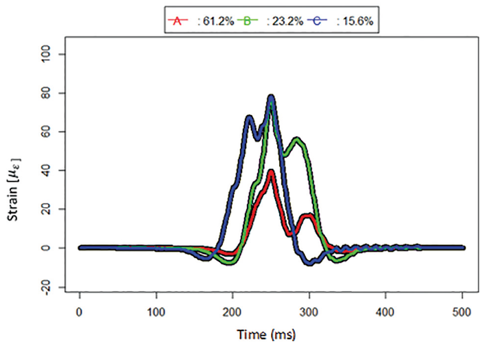
Clustering output with three clusters.

Step 2: Truck Classification—Image Visual Inspection

Forty-three photos of trucks crossing the bridge were analyzed. These images are used to associate the type of truck to its corresponding cluster. Some challenges are attributable to the images only showing the front of the truck, not its whole length, in addition to the lack of information on whether or not all the other regular trucks are traveling empty or just with a light load. The image visual inspection revealed the following qualitative classification of the trucks, listed below and summarized in Table 1.

Table 1.

Summary of Truck Characteristics Within Each Strain Cluster

Cluster	Sub-cluster	Truck type	Weight	Waveform	Class
A→ 67.44% (29)	A1	Tank trucks	Light	Bimodal	9
	A2	Flatbed	Medium-light	Bimodal	9–10
	A3	Regular trucks	Light	Bimodal	9
	A4	Regular trucks	Medium	Bimodal	9–10
B → 20.93% (9)	B1	Logging trucks	Heavy/overweight	Non-bimodal	12
B → 20.93% (9)	B2	Regular trucks	Heavy	Bimodal	9
C → 11.63% (5)	C	Logging trucks	Heavy/overweight	Non-bimodal	12

Cluster A presents bimodal waveforms and is generated by trucks with the following characteristics: lighter GVW (always below the 80-kip limit), the presence of a large spacing (25–30 ft) usually between axle 3 and 4. These trucks are:

Tank trucks with GVW ≤ 40 kip (18 tons), Class 9, all with identical axle configuration.

Flatbed, empty, or light weighted, with GVW ≤ 50 kip (∼22 tons) or just slightly above 50 kip (23 tons); class 9 (five axles) and 10 (six axles). Sometimes they can be confused with empty logging trucks; however, their axle’s configurations clearly differ.

Regular trucks with GVW < 50 kip (23 tons), suggesting partial or lightweight cargo or empty; class 9.

Regular trucks with GVW between 50 (23 tons) and 70 kip (32 tons); class 9 and 10.

Cluster B presents two different waveforms, a bimodal and non-bimodal one, and it is generated by heavy trucks, often overweight. These trucks are:

Full logging trucks, GVW is about 100 kip (45 tons) or more; class 12 (six axles); axles more equally spaced although there is at least one larger spacing between axles 3 and 4 of 12–18 ft (3.7–5.5 m); they present a non-bimodal waveform.

Regular trucks with high GVW, sometimes overweight but never reaching 100 kip (45 tons); class 9; they present a bimodal waveform because of the spacing, often larger than 25 ft (7.6 m).

Cluster C presents mostly non-bimodal waveforms and it is generated by extremely heavy trucks, most of the time overweight. These trucks are:

Full logging trucks, GVW is about 100 kip (45 tons) or more; class 12 (six axles); axles more equally spaced although there is still a large spacing between axles 3 and 4 of 12–18 ft (3.7–5.5 m); they present a non-bimodal waveform.

The image visual inspection provides the important contribution to assigning a truck type to each cluster and confirms what is the correct number of clusters. The best option identified in the first iteration of step 1 was three clusters; however, the results shown in Table 1, supported by images, suggest that four clusters might be a more accurate choice as it seems that cluster B can be split into two different clusters and A4 can be better allocated to cluster B since it seems to be slightly borderline in cluster A. Based on these considerations, a new iteration of Step 1 is performed.

Step 1: Clustering of Bridge Response (Iteration 2)

The results of the longitudinal clustering analysis considering four clusters are shown in Figure 6. The clustering analysis in the second iteration confirms considerations made previously, such as the presence of two different types of trucks in cluster B (B1: logging trucks; B2: heavy bimodal trucks), which, in the four-cluster option, are split with more accuracy into two different clusters: B (heavy bimodal) and C (logging non-bimodal). Type A4 is also reassigned from cluster A (three-cluster option) to cluster B (four-cluster option) with other heavier trucks, which cause bimodal responses. This reassignment is reasonable given its higher GVW compared to the other trucks within the same cluster. The reorganization of trucks into for clusters, shown in Figure 7, completes step 1.

Figure 6.

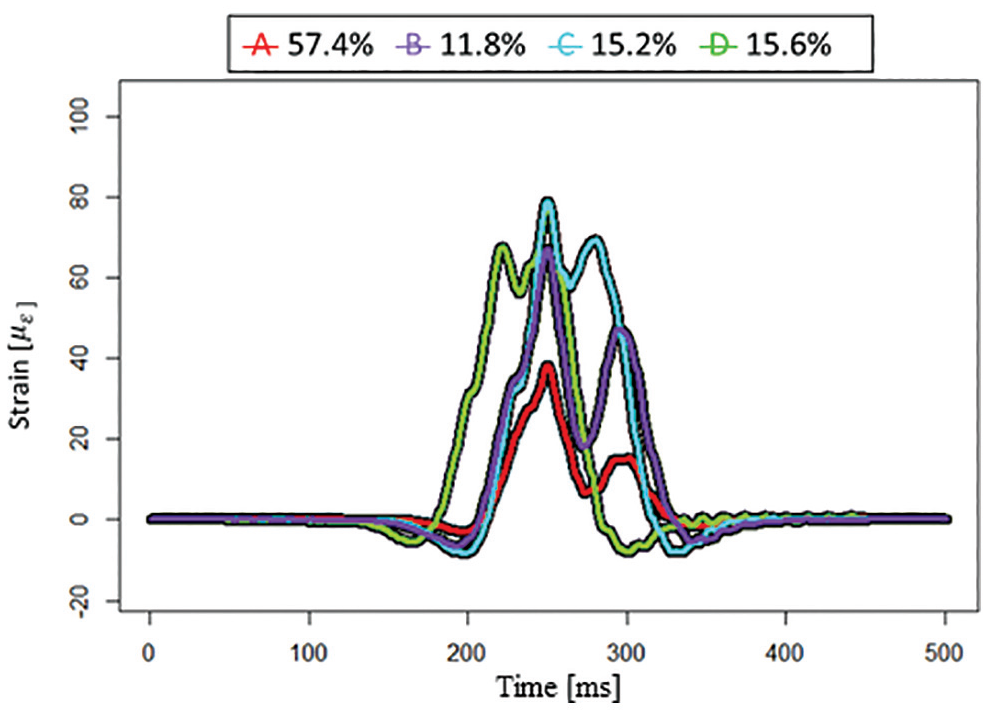
Clustering output with four clusters.

Figure 7.

Cluster reassignment.

Step 2: Truck Classification—Classification Tree

Step 2 presents the results of the classification tree (Figure 8), where it is clear that the first split is governed by GVW, which divides lighter trucks (A) from heavy trucks (B, C, and D). The second split separates heavy trucks according to the shape of their waveform (bimodal B or mostly not bimodal C, D), which is strictly connected to the dimension of spacing between axles 3 and 4. A large spacing indicates a bimodal waveform, meaning that after axle 3 hits the bridge there is enough time for the bridge response to reach low values of strain again before axle 4 hits the bridge. Finally, the heavy trucks with more equally spaced axles (clusters C and D) are separated by the weight of axle 6, with D having a heavier rear axle than C. The two-step algorithm has finally clustered the bridge responses and assigned a truck profile to each of them. These results will be used to build the classification framework for the Hurley Bridge.

Figure 8.

Classification tree with four clusters.

Classification Framework

The classification framework collects and organizes all the results from the calibration of the two-step algorithm (Table 2). Its categories (type of waveform, type of trucks, weight classes, axle configuration, etc.) are strictly related to the specific bridge, its traffic, and the surrounding environment and activities; therefore, they can be customized. For example, the presence of logging trucks was a distinctive characteristic that made Hurley Bridge the ideal candidate to show the practical importance of this work as these vehicles have great potential to cause harm to the structure. However, not all bridges face this challenge. Table 2 shows a possible template of the classification framework with the essential information necessary, where the cluster letter can be replaced with the actual waveform. Its structure can be fully customized depending on the decision-maker’s goals and needs, by adding other relevant information such as axle configuration (see step 2 of the two-step algorithm for suggestions).

Table 2.

Classification Framework

Bridge			Truck
Cluster	Waveform	Peak strain	Truck type	Weight	FHWA class
A	Bimodal	<50 µε	Tank truck	Light	9
				≤40 kip	9
A	Bimodal	<50 µε	Flatbed truck	Medium-light	9–10
				≤70 kip	9–10
A	Bimodal	<50 µε	Regular truck	Light	9
				≤50 kip	9
B	Bimodal	≥50–80 µε	Regular truck	Medium-heavy	9–10
				≥50 kip	9–10
C	Non-bimodal	≥80 µε*	Logging truck	Heavy/overweight	12
				≥80 kip (heavier front)	12
D	Non-bimodal	≥80 µε*	Logging truck	Heavy/overweight	12
				≥80 kip(heavier rear)	12

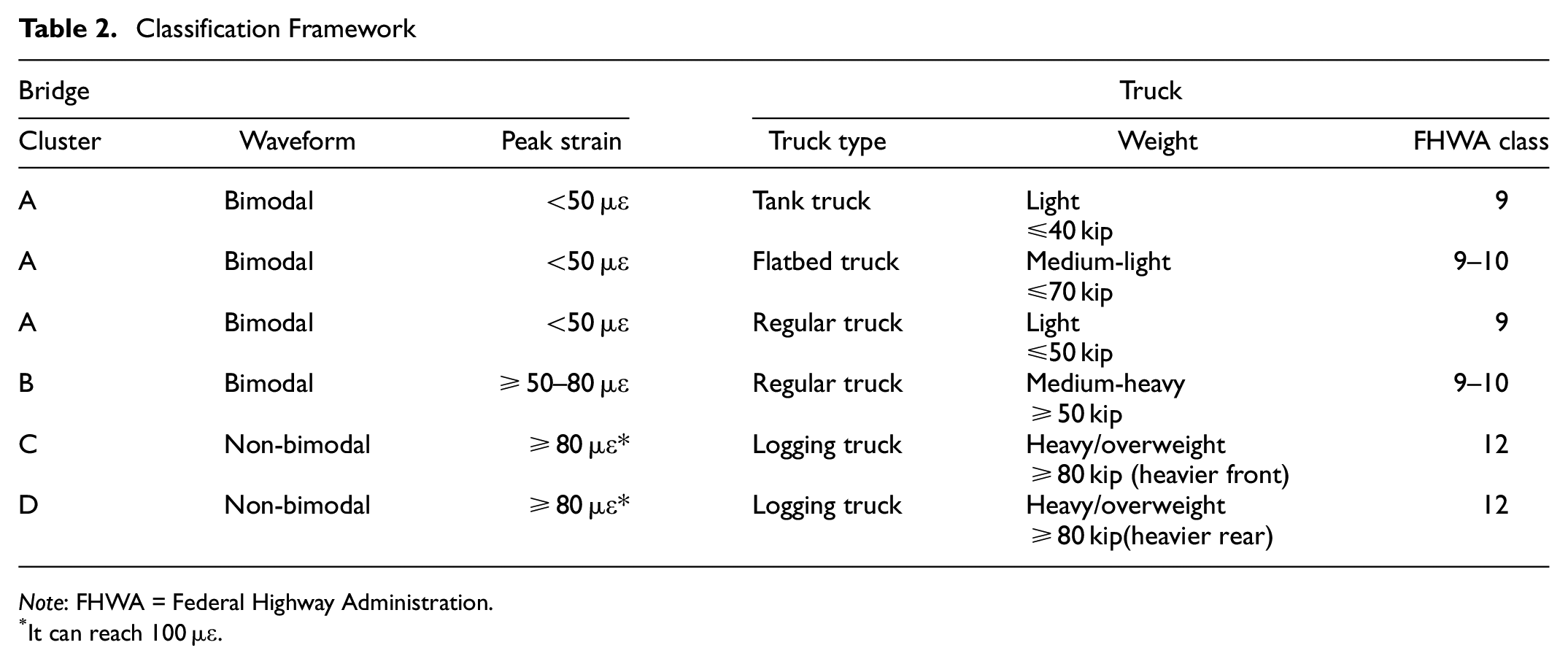
Note: FHWA = Federal Highway Administration.

It can reach 100 µε.

Use Cases

The use cases of the classification framework and the two-step algorithm presented here describe real-life situations that bridge owners, bridge managers, local authorities, and policymakers may face. Use cases 1 and 2 show how the classification framework fills the gap when one monitoring system is discontinued. Use case 3 presents an example of how this work can support decision-makers in flagging potentially dangerous heavy trucks. The two-step algorithm can also be used as a standalone tool when data can be collected from both monitoring systems. Use cases 4 and 5 are examples of how policymakers can also benefit from the two-step algorithm to regulate heavy trucks that access aging structures. Periodical calibrations of the two-step algorithm can be performed to create benchmarks that provide the user with valuable insights on how the bridge is performing and whether or not its traffic is changing (use case 6). Monthly and yearly comparisons are pivotal in the long-term monitoring of any structure.

Use Case 1: Classification Framework, Truck to Bridge

Because of the frequent need for maintenance and upgrades, the structural health system installed on the bridge is discontinued. The WIM system, however, is still functioning and keeps collecting information about the trucks that regularly cross the bridge. Figure 9 shows how, given the truck’s characteristics captured by the WIM system, the classification framework returns an estimate of the strain waveform that the truck might generate.

Figure 9.

Estimate of strain waveform given truck’s information.

Use Case 2: Classification Framework, Bridge to Truck

Some components of the WIM systems are damaged by the heavy traffic and, as a result of lack of resources, they cannot be replaced or fixed. The SHM system, however, remains functional and it records strain responses of the bridge at each truck crossing. Figure 10 shows how the classification framework intakes the strain waveform recorded by the SHM system and returns a potential profile of the truck which generated that waveform.

Figure 10.

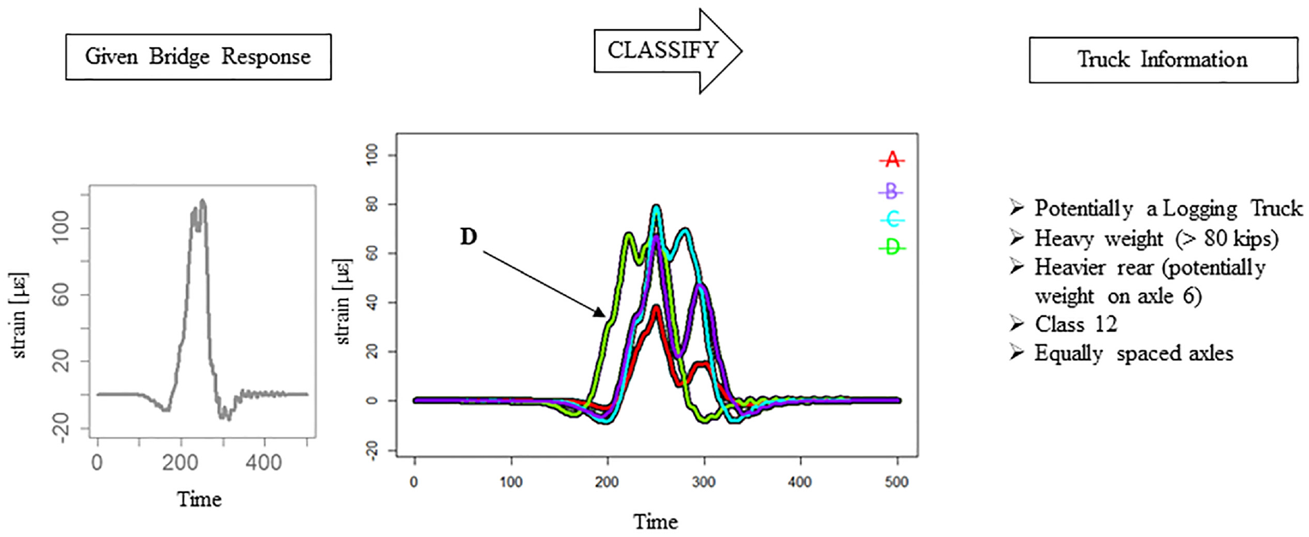
Identification of truck’s profile given the bridge strain waveform generated.

Use Case 3: Classification Framework, Red Flags

Decision-makers need to have a clear picture of the interaction between the bridge and its heavy traffic. The information provided by the classification framework (Table 2) can highlight which types of trucks should be taken under control. GVW and axle configuration are the truck’s characteristics that play a key role in defining how the bridge responds with regard to strain. Trucks in cluster A are considered the least dangerous, with a strain response that never exceeds 50 µε. Even if they present a bimodal strain waveform, caused by the presence of a large spacing, typical of class 9 trucks, their moderate weight assures their allocation among the safer traffic of this bridge. Trucks in cluster B are much heavier than A and often overweight (80-kip limit); in addition, they also present a bimodal waveform as a result of at least one large spacing between axles. This axle configuration makes the bridge perceive one truck crossing as almost two, which, in addition to the heavyweight, would speed up fatigue damages in areas that are particularly prone to it. Clusters C and D group logging trucks, which are a constant presence on the Hurley bridge. These two clusters show a very high GVW, sometimes exceeding 100 kip (45 tons) (limit 98 kip on six axles). The concern is because of the peak strain that they can reach, which is up to 100 µε and more. They differ from each other in how the weight is allocated. Unlike trucks in cluster A, trucks which fall in cluster B, C, and D should all be taken under control to mitigate potential problems to the bridge and its components. In addition to regular trucks, although very limited in number, there are cases of vehicles with special features or cargo where the bridge response can reach up to 250 µε. This use case sheds a light on how this work can also aid policymakers in adjusting some policies to manage those type of trucks that can be harmful to the bridge, not by only considering GVW or axle configuration individually, but the combination of the two. For instance, the GVW limit on some highways is set to 80 kip (∼36 tons), but there are some trucks in cluster B with GVW lower than the limit, which can still be harmful because of their axle configuration.

Use Case 4: Two-step Algorithm, Truck Frequency

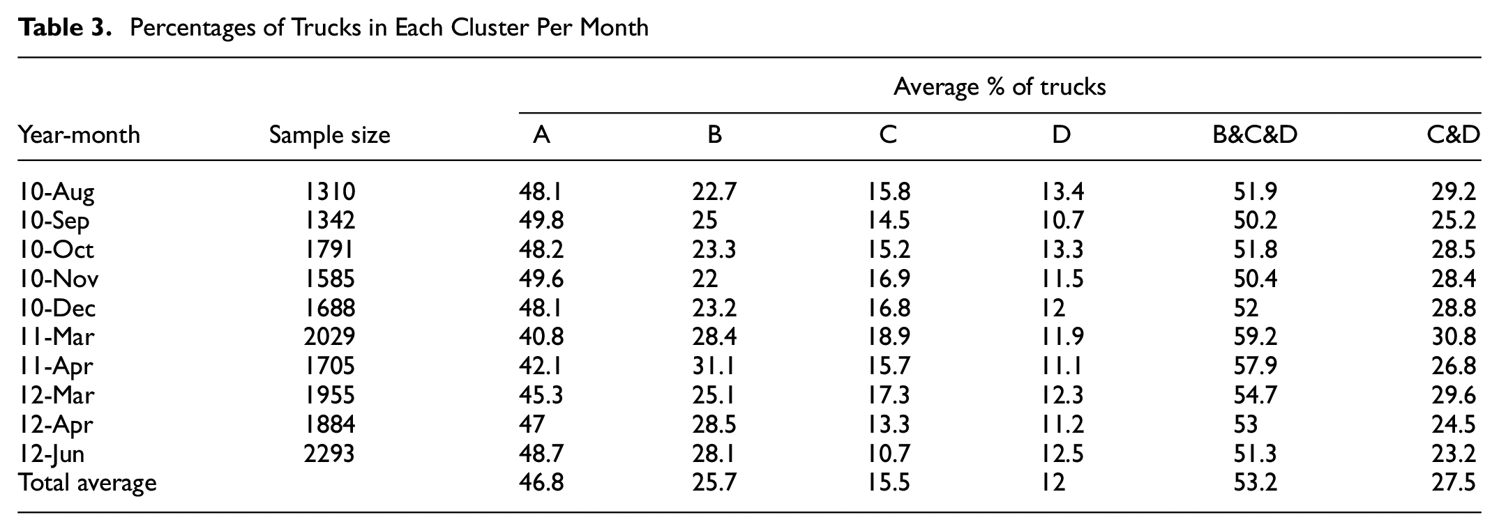
Once the effects of the trucks that routinely cross the bridge are identified, it becomes crucial to monitor the frequency of those trucks which are potentially more harmful to the bridge. Over a three-year period, 10 months of strain and traffic data are selected for their significant sample size, and four clusters are considered for each month. Table 3 shows the monthly average of the percentage of trucks that fall in each cluster. Trucks in cluster A are always between 40% and 50%, and they represent the majority of trucks, which might seem encouraging because, according to the discussion in the previous section, cluster-A trucks are the lightest and the least harmful among the heavy trucks. For comparison purposes, it is important to combine the heavier clusters in at least two scenarios: (i) B&C&D combines all the heavier trucks; and (ii) C&D combines all the logging trucks to better understand the magnitude of the logging activity. The results show that all heavy trucks (B, C, and D) are slightly more than 50%, with the most common type of truck being the logging truck (C and D), which are slightly less than 30% of the whole truck traffic. Less numerous than logging trucks are trucks belonging to cluster B, which present a peak of 30% in April 2011. This peak could be down to the Wisconsin statutory change ( 29 ), which allowed heavy trucks to cross the area even during the spring thaw. Overall, the percentage of trucks for each type is stable and quite constant over the studied period.

Table 3.

Percentages of Trucks in Each Cluster Per Month

Year-month	Sample size	Average % of trucks
		A	B	C	D	B&C&D	C&D
10-Aug	1310	48.1	22.7	15.8	13.4	51.9	29.2
10-Sep	1342	49.8	25	14.5	10.7	50.2	25.2
10-Oct	1791	48.2	23.3	15.2	13.3	51.8	28.5
10-Nov	1585	49.6	22	16.9	11.5	50.4	28.4
10-Dec	1688	48.1	23.2	16.8	12	52	28.8
11-Mar	2029	40.8	28.4	18.9	11.9	59.2	30.8
11-Apr	1705	42.1	31.1	15.7	11.1	57.9	26.8
12-Mar	1955	45.3	25.1	17.3	12.3	54.7	29.6
12-Apr	1884	47	28.5	13.3	11.2	53	24.5
12-Jun	2293	48.7	28.1	10.7	12.5	51.3	23.2
Total average		46.8	25.7	15.5	12	53.2	27.5

Use Case 5: Two-Step Algorithm, Peak Strain

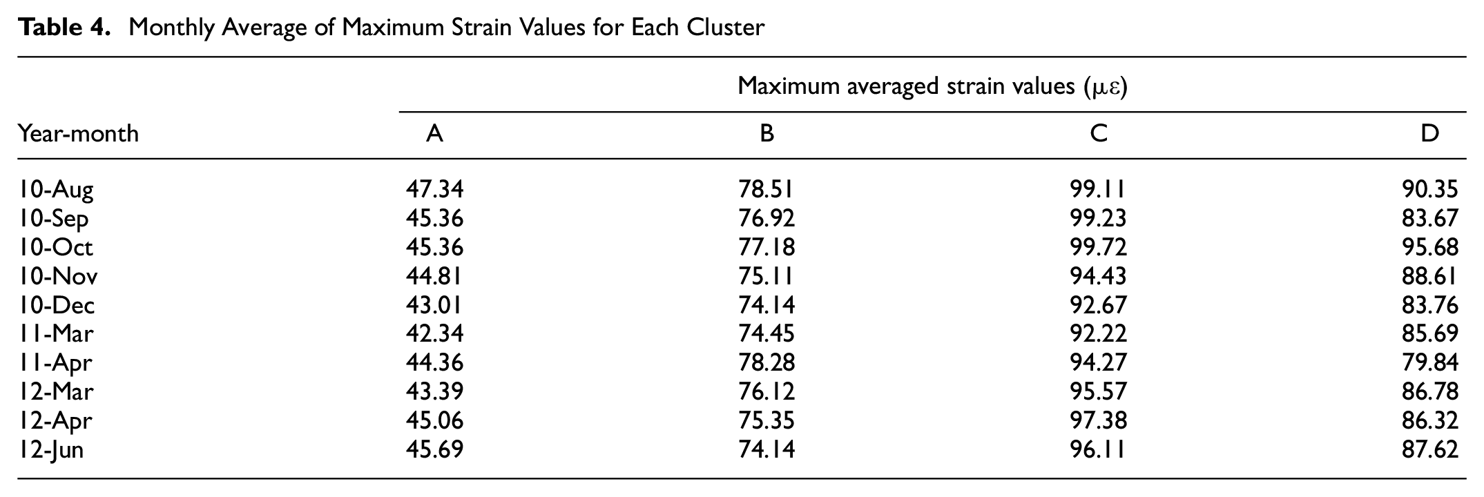
It is also crucial to monitor the maximum recorded strain the bridge underwent. Table 4 shows how the average of all maxima in each month for all clusters is quite stable over time, with small variations during some months. The highest averaged value of strain reported belongs to cluster C (99.72 µε). Some months showed waveforms that exceeded 200 µε, mainly caused by FHWA class 13 trucks with nine axles, whose frequency should be taken under control over time. Because of their limited number, the presence of these extreme events did not alter the average values of all waveforms shown in the table. If outliers become more frequent, the average values will be affected, and this shift can be used as an early warning for the bridge safety.

Table 4.

Monthly Average of Maximum Strain Values for Each Cluster

Year-month	Maximum averaged strain values (µε)
	A	B	C	D
10-Aug	47.34	78.51	99.11	90.35
10-Sep	45.36	76.92	99.23	83.67
10-Oct	45.36	77.18	99.72	95.68
10-Nov	44.81	75.11	94.43	88.61
10-Dec	43.01	74.14	92.67	83.76
11-Mar	42.34	74.45	92.22	85.69
11-Apr	44.36	78.28	94.27	79.84
12-Mar	43.39	76.12	95.57	86.78
12-Apr	45.06	75.35	97.38	86.32
12-Jun	45.69	74.14	96.11	87.62

Use Case 6: Two-Step Algorithm, Benchmarks

To assess how the bridge-traffic system evolves over time, it is common practice to compare the current state with some benchmark values. Figures 11 and 12 show a comparison between two consecutive months and two consecutive years. The first comparison is between March 2012 and April 2012 (Figure 11), where four splits of the classification tree remained the same over time with negligible differences in the following values: GVW, which splits all trucks in lighter and heavy; spacing 3–4, which split bimodal from non-bimodal waveforms; speed which separates A from B, also in the heavier side of GVW; length which separates D from C. The remaining splits are also related to each other—for example, axle weight 4 in March 2012 and GVW in April 2012 agree that weight is influencing this split; spacing 2–3 and axle weight 1, even if they are different quantities with different units are both related to the front part of the truck. The second comparison is between two consecutive years (March 2011 and March 2012), as shown in Figure 12. It is encouraging to see how the most important parameters which constitute the structure of the tree (GVW, spacing 3–4, speed, and length) are consistent, suggesting the reliability of this method to classify and monitor trucks over time.

Figure 11.

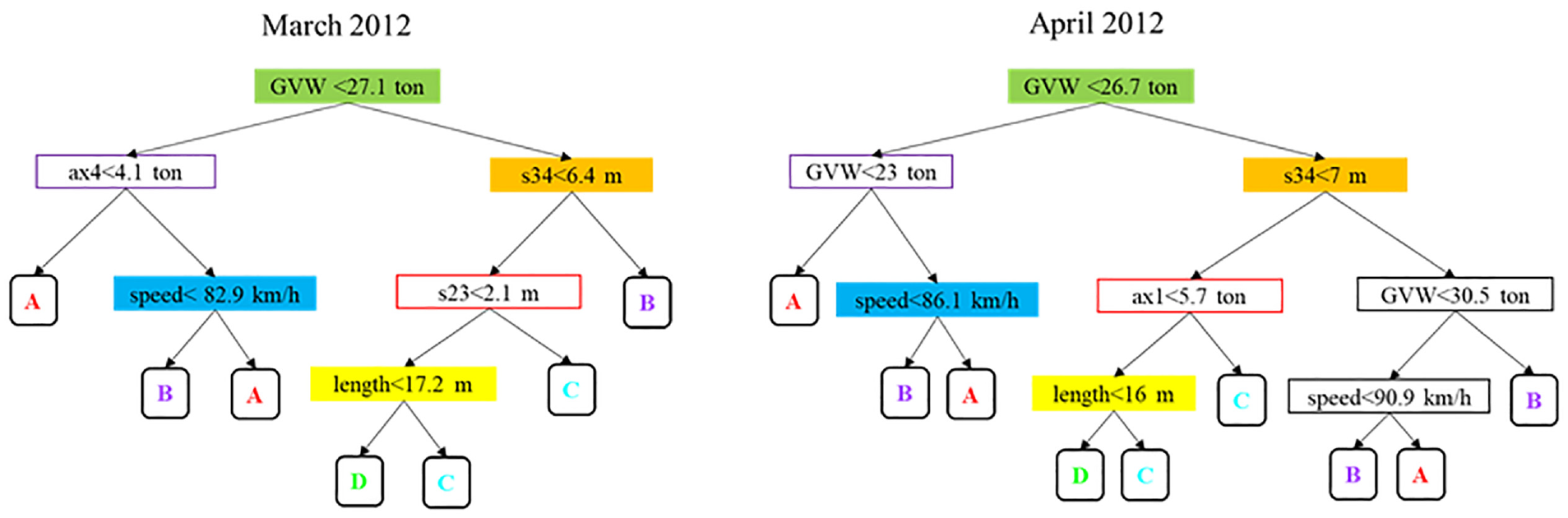
Comparison of two consecutive months.

Figure 12.

Comparison of two consecutive years.

Results and Discussion

The results of the calibration of the two-step algorithm used to build the classification framework for the Hurley bridge (Table 2) and some important considerations drawn from the use cases are outlined in this section. The heavy traffic that routinely crosses the bridge consists of three main categories—light, heavy, and logging trucks—and, more specifically, the bridge presents four different types of strain responses (clusters)—bimodal waveform/lower strain, bimodal/higher strain, and non-bimodal/very high strain, with different weight distributions. The respective peak strain ranges from below 50 µε, between 50 and 80 µε, and up to 100 µε, especially during logging season. The FHWA classes 9 and 10 are more likely to result in a bimodal response of the bridge, while class 12 usually generates a non-bimodal one.

Monitoring the frequency of the trucks in each cluster can support a more durable life cycle of the structure. It is also crucial to monitor the frequency of extreme peak strains that they produce, which, however, are not solely responsible for the structural deterioration and fatigue damages. It is demonstrated how trucks that produce a bimodal strain waveform can have a non-negligible role in accelerating the aging process of the structure because one crossing is, in practice, perceived by the bridge as almost two.

It is good practice to perform periodical benchmarks, that, if regularly performed, can be useful to monitor how known issues evolve and to help to reveal problems that are not easily detectable during a bridge visual inspection because of potential difficulties reaching the site or less frequent inspections.

Conclusions and Future Work

The present work contributes to the subject of long-term monitoring of bridges and heavy traffic by presenting a solution to be adopted when either the bridge or the traffic is no longer monitored. This paper proposed a two-step algorithm which utilized longitudinal clustering (step 1), where the bridge responses are grouped into a finite number of categories; and image processing and classification tree (step 2), where each truck crossing the bridge is assigned to one of the cluster categories from step 1. To calibrate the two-step algorithm, it was necessary to collect data from both the bridge and the traffic for a limited, yet significant, amount of time. The results of the two-step algorithm were then used to build a classification framework that allowed identification of the profile of the truck crossing the bridge by only knowing the bridge response or the estimate of the bridge response by knowing the truck’s characteristics. The bridge response is categorized according to the shape of strain waveform and peak strain, while trucks are classified by type and truck’s characteristics.

A complete proof of concept, using the Hurley bridge data, of the proposed solution was developed to demonstrate its feasibility. Four types of bridge responses were identified by the algorithm. Bridge response A showed a bimodal strain waveform and a relatively low peak strain; the trucks that are crossing the bridge have a light to medium weight, FHWA class 9 or 10. Bridge response B showed similar characteristics to cluster A, such as the bimodal strain response and the types of trucks; however, the weight and, therefore, the peak strain were higher than cluster A. Bridge responses C and D were generated by the logging trucks, FHWA class 12, that routinely cross the bridge. They did not generate a bimodal strain waveform but, as a result of their significantly high weight, their peak strain can reach extremely high values. The difference between these two responses was caused by different weight distributions.

Overall, the classification framework provides the advantages of two monitoring systems while, in reality, only one is active. Multiple use cases were also presented to validate its real-life applicability and to emphasize the value it can bring to decision-makers such as bridge managers, practitioners, policymakers, and local authorities by allowing them to make more data-driven decisions based on detailed analyses, which can be pivotal in extending the lifespan of aging bridges.

The limitations of the proposed study are interesting opportunities for future research. The methodology for outlier detection can be further improved; the presence of multiple vehicles can be added to the present study; the use of more advanced image processing techniques based on machine learning, like SVMs, artificial neural networks, decision tree, and K-nearest neighbor, or deep learning like a convolutional neural network, can be explored to fully computerize the methodology; and, finally, since the proposed methodology can be widely applicable to any monitored bridge and its traffic, other calibrations should follow in each specific test bed.

Footnotes

Acknowledgements

The support of the Wisconsin Department of Transportation, including the provision of access to the bridge, data communication, and access to WIM data, as well as consultation and advice, is gratefully acknowledged. The authors also wish to acknowledge the efforts of former NU-ITI engineers David Kosnik, Daniel Marron, and Mathew Kotowsky for their critical roles in instrumentation, data acquisition, and communication for the bridge.

Author Contributions

The authors confirm contribution to the paper as follows: study conception and design: Fiorella Mete, David J. Corr, Ying Chen; data collection: David J. Corr; analysis and interpretation of results: Fiorella Mete, Ying Chen, David J. Corr; draft manuscript preparation: Fiorella Mete, David J. Cor, Ying Chen, Michael P. Wilbur. All authors reviewed the results and approved the final version of the manuscript.

Declaration of Conflicting Interests

The authors declared no potential conflicts of interest with respect to the research, authorship, and/or publication of this article.

Funding

The authors received no financial support for the research, authorship, and/or publication of this article.

ORCID iDs

Michael P. Wilbur

Ying Chen

References

Fiorillo

Ghosn

Procedure for Statistical Categorization of Overweight Vehicles in a WIM Database. Journal of Transportation Engineering, Vol. 140, No. 5, 2014, p. 04014011.

Wang

T.-L.

Liu

Influence of Heavy Trucks on Highway Bridges. Final Report. Florida Department of Education, Tallahassee, FL, 2000.

Luskin

Walton

C. M.

Effects of Truck Size and Weights on Highway Infrastructure and Operations: A Synthesis Report. Technical Report. Center for Transportation Research, Bureau of Engineering Research, University of Texas at Austin, 2001.

Sun

Ritchie

S. G.

Inductive Classifying Artificial Network for Vehicle Type Categorization. Computer-Aided Civil and Infrastructure Engineering, Vol. 18, No. 3, 2003, pp. 161–172.

Battiato

Farinella

G. M.

Furnari

Puglisi

Snijders

Spiekstra

An Integrated System for Vehicle Tracking and Classification. Expert Systems with Applications, Vol. 42, No. 21, 2015, pp. 7263–7275.

Mosa

A. H.

Kyamakya

Junghans

Ali

Al Machot

Gutmann

Soft Radial Basis Cellular Neural Network (SRB-CNN) Based Robust Low-Cost Truck Detection Using a Single Presence Detection Sensor. Transportation Research Part C: Emerging Technologies, Vol. 73, 2016, pp. 105–127.

Simoncini

Taccari

Sambo

Bravi

Salti

Lori

Vehicle Classification from Low-Frequency GPS Data with Recurrent Neural Networks. Transportation Research Part C: Emerging Technologies, Vol. 91, 2018, pp. 176–191.

Zhang

Wang

Suo

A Novel Vehicle Classification Using Embedded Strain Gauge Sensors. Sensors, Vol. 8, No. 11, 2008, pp. 6952–6971.

Yan

Fraser

Elgamal

Fountain

Oliver

Neural Networks and Principal Components Analysis for Strain-Based Vehicle Classification. Journal of Computing in Civil Engineering, Vol. 22, No. 2, 2008, pp. 123–132.

10.

Shim

Chung

Choi

I.-C.

A Comparison Study of Cluster Validity Indices Using a Nonhierarchical Clustering Algorithm. Proc., International Conference on Computational Intelligence for Modelling, Control and Automation, 2005 and International Conference on Intelligent Agents, Web Technologies and Internet Commerce, No. 1, Vienna, Austria, IEEE, New York, NY, 2005, pp. 199–204.

11.

Wheeler

A. P.

Worden

R. E.

McLean

S. J.

Replicating Group-Based Trajectory Models of Crime at Micro-Places in Albany, NY. Journal of Quantitative Criminology, Vol. 32, No. 4, 2016, pp. 589–612.

12.

Charlton

R. A.

Neville

A. J.

Jordan

Pierini

Damase-Michel

Klungsøyr

Andersen

A. M. N.

Hansen

A. V.

Gini

Bos

J. H.

Healthcare Databases in Europe for Studying Medicine Use and Safety During Pregnancy. Pharmacoepidemiology and Drug Safety, Vol. 23, No. 6, 2014, pp. 586–594.

13.

Laurin

J. C.

Geoffroy

M.-C.

Boivin

Japel

Raynault

M.-F.

Tremblay

R. E.

Côté

S. M.

Child Care Services, Socioeconomic Inequalities, and Academic Performance. Pediatrics, Vol. 136, No. 6, 2015, pp. 1112–1124.

14.

Herba

C. M.

Glover

Ramchandani

P. G.

Rondon

M. B.

Maternal Depression and Mental Health in Early Childhood: An Examination of Underlying Mechanisms in Low-Income and Middle-Income Countries. The Lancet Psychiatry, Vol. 3, No. 10, 2016, pp. 983–992.

15.

Pingault

J.-B.

Côté

S. M.

Galéra

Genolini

Falissard

Vitaro

Tremblay

R. E.

Childhood Trajectories of Inattention, Hyperactivity and Oppositional Behaviors and Prediction of Substance Abuse/Dependence: A 15-Year Longitudinal Population-Based Study. Molecular Psychiatry, Vol. 18, No. 7, 2013, p. 806.

16.

Mete

Chen

Stathopoulos

Corr

D. J.

Comparative Study of Predictive Analysis Methods to Estimate Bridge Response. Transportation Research Record: Journal of the Transportation Research Board, 2019. 2673(9): 365–376.

17.

Erman

Arlitt

Mahanti

Traffic Classification Using Clustering Algorithms. Proc., 2006 SIGCOMM Workshop on Mining Network Data, Pisa, Italy, ACM, New York, NY, 2006, pp. 281–286.

18.

Jeng

S.-T.

Ritchie

Real-Time Vehicle Classification Using Inductive Loop Signature Data. Transportation Research Record: Journal of the Transportation Research Board, 2008. 2086: 8–22.

19.

Hernandez

S. V.

Tok

Ritchie

S. G.

Integration of Weigh-in-Motion (WIM) and Inductive Signature Data for Truck Body Classification. Transportation Research Part C: Emerging Technologies, Vol. 68, 2016, pp. 1–21.

20.

Van Cranenburgh

Wang

Vij

Pereira

Walker

Choice Modelling in the Age of Machine Learning. arXiv Preprint arXiv:2101.11948, 2021.

21.

Genolini

Falissard

KmL: k-means for longitudinal data. Computational Statistics, Vol. 25, No. 2, 2010, pp. 317–328.

22.

Caliński

Harabasz

A Dendrite Method for Cluster Analysis. Communications in Statistics-Theory and Methods, Vol. 3, No. 1, 1974, pp. 1–27.

23.

Salzberg

S. L.

Book Review: C4. 5: Programs for Machine Learning by J. Ross Quinlan. Morgan Kaufmann Publishers, Inc., 1993. Kluwer Academic Publishers, Boston, MA, 1994.

24.

Kumar

Quinlan

J. R.

Ghosh

Yang

Motoda

McLachlan

G. J.

Liu

Philip

S. Y.

Top 10 Algorithms in Data Mining. Knowledge and Information Systems, Vol. 14, No. 1, 2008, pp. 1–37.

25.

Ritschard

Computing and Using the Deviance with Classification Trees. In COMPSTAT 2006-Proceedings in Computational Statistics ( Rizzi

Vichi

, eds.), 2006, Springer, Germany, pp. 55–66.

26.

Kosnik

D. E.

Zhang

Durango-Cohen

P. L.

Application of Statistical Process Control for Structural Health Monitoring of a Historic Building. Journal of Infrastructure Systems, Vol. 20, No. 1, 2013, p. 05013002.

27.

Ghasemi

S. H.

Nowak

A. S.

Parastesh

Statistical Parameters of In-A-Lane Multiple Truck Presence and a New Procedure to Analyze the Lifetime of Bridges. Structural Engineering International, Vol. 26, No. 2, 2016, pp. 150–159.

28.

Hosseini

Ghasemi

S. H.

Jalayer

Nowak

A. S.

Performance-Based Reliability Analysis of Bridge Pier Subjected to Vehicular Collision: Extremity and Failure. Engineering Failure Analysis, Vol. 106, 2019, p. 104176.

29.

Owusu-Ababio

Schmitt

Evaluation of Impacts of Allowing Heavier Log Loads in Northern Wisconsin During Spring Thaw. Wisconsin Highway Research Program. Wisconsin Department of Transportation, Madison, 2014.