
Abstract
We propose a bilevel transit network frequency setting problem in which the upper level consists of analytical route cost functions and the lower level is an activity-based market equilibrium derived using MATSim-NYC. The use of MATSim in the lower-level problem incorporates sensitivity of the design process to competition from other modes, including ride-hail, and can support large-scale optimization. The proposed method is applied to the existing Brooklyn bus network, which includes 78 bus routes, 650,000 passengers per day, 550 route-km, and 4,696 bus stops. MATSim-NYC modeling of the existing bus network has a ridership-weighted average error per route of 21%. The proposed algorithm is applied to a benchmark network and confirms their predicted 20% growth in ridership using their benchmark design. Applying our proposed algorithm to their network with 78 routes and 24 periods, we have a problem with 3,744 decision variables. The algorithm converged within 10 iterations to a delta of 0.064%. Compared with the existing scenario, we increased ridership by 20% and reduced operating cost by 25%. We improved the farebox recovery ratio from the existing 0.22 to 0.35, 0.06 more than the benchmark design. Analysis of mode substitution effects suggest that 2.5% of trips would be drawn from ride-hail while 74% would come from driving.
Keywords
Despite the emergence of many new mobility options in cities around the world, fixed route transit is still the most efficient means of mass transport ( 1 ). This is evident to mobility providers as well as companies like Uber who experiment with “cheaper fares in exchange for more walking” ( 2 ). Transit efficiency, however, is well known to be interdependent with ridership demand and network design ( 3 – 9 ).
Bus operations are subject to vicious and virtuous cycles ( 10 ). Evidence of this can be seen in New York City (NYC). Since 2007, travel speed reductions and increased congestion as a result of more mobility options competing for road space have led to a vicious cycle of ridership reduction and further increased congestion as former transit passengers take to other less congestion-efficient modes. In Brooklyn, bus ridership has declined by 21% during this period. While the decrease in ridership has been steady throughout this period, there is an emerging concern that it will only get worse as for-hire vehicle services like Uber and Lyft add more trips to the road network ( 11 ). Clewlow and Mishra ( 12 ) find that 49% to 61% of ride-hailing trips are substituting from walking, biking, or transit trips.
Intervention in the form of network redesign is required to promote a virtuous cycle and make the bus more competitive, especially in the face of increased competition from ride-hail services ( 13 ). This can be done by redesigning the bus network in a way that reduces operating and user costs while increasing accessibility for more riders. Methods to systematically improve a transit network fall into the class of transit network design problems (NDPs) (see Guihaire and Hao [ 14 ]).
The research gap suggests that transit NDPs lack consideration of the sensitivity of a design to competition from other modes like ride-hail. Studies have considered transit design strategies like frequency setting or route setting that model elastic demand through mode and route choice equilibrium as a Stackelberg game. However, none of these studies have considered traveler response from an activity-based travel perspective. One exception is Li et al. ( 15 ) which used a lower-level quasi-dynamic user equilibrium in a time-space network, but it did not include other modes like driving alone, carpool, taxi, ride-hail, bike-share, and walking. As a result, the activity-based demand does not capture elasticity to choose other mode choices. It also could not scale to realistic size problems. Another group ( 16 – 18 ) explored metaheuristics to design a network subject to MATSim-simulated activity behavioral responses. The latter research uses computationally efficient tools for large-scale modeling of activity-based demand responses from travelers which can incorporate mode competition. However, those latter studies did not formalize a transit network design model with an upper-level model to find the best design decisions, relying instead solely on stochastic search algorithms like genetic algorithms (GA). The problem is that metaheuristics like GA alone may not exploit the problem structure, which can be computationally inefficient for NDPs (see Chow et al. [ 19 ]), although some implementations have been quite effective ( 20 – 23 ).
We propose a transit network design framework in which analytical route cost models, as shown in Tirachini ( 24 ), are used in an upper level of a bilevel optimization problem with a MATSim lower-level response. An iterative algorithm is implemented to solve the problem. The model therefore combines techniques from both analytical and simulation-based tools. To the best of our knowledge, no study has proposed such a bilevel transit network design problem.
Literature Review
Transit Network Frequency Setting
There are four main activities in public transportation planning: network route design, timetable development, vehicle scheduling, and crew scheduling. Strategic planning involves planning routes and frequencies, often called the line planning problem. Hasselström ( 25 ) and Van Nes et al. ( 26 ) proposed early line planning optimization models for setting frequencies as the only decision variables. More recent studies that consider both route design and frequency setting include Chu ( 27 ), Cancela et al. ( 28 ), and Szeto and Wu ( 29 ). Reviews of transit network design models and algorithms can be found in Desaulniers and Hickman ( 7 ), Guihaire and Hao ( 14 ), and more broadly in Farahani et al. ( 30 ). Line planning has been shown to be NP-hard in complexity (see Schöbel and Scholl [ 31 ]) leading to the use of route construction heuristics as in Ceder and Wilson ( 6 ).
For those interested in optimizing more custom designs, researchers have proposed continuous approximation models to evaluate homogeneous transit network designs; for example, Newell ( 5 , 32 ) and Byrne ( 33 ). The optimal frequency is found to be proportional to the square root of the arrival rate of passenger and sometimes referred to as the “square root rule.” Mohring ( 4 ) independently showed a similar square-root rule using a simpler construct of the cost function.
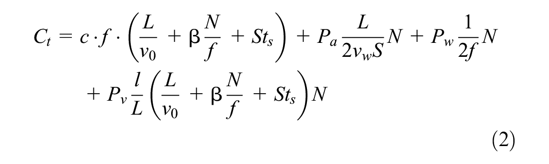
Analytical models of this square-root form are still of use to contemporary researchers. Tirachini ( 24 ) provides a simple analytical approach by considering operational cost, user waiting cost, user access and egress cost, and in-vehicle time cost. The total cost function is shown in Equations 1 and 2.
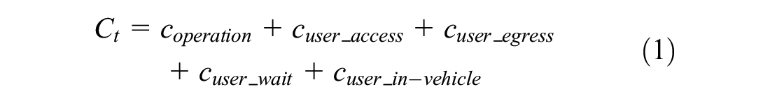
where
Bilevel Transit Frequency Setting Algorithms
Bilevel NDPs refer to an optimization problem divided into two levels (see Chow [ 34 ]). At the upper level a decision maker determines design variables for a system in anticipation of the reaction of the users. At the lower level, users have an objective that is separate from the upper-level objective which decides the decision variables used for the upper-level problem. An optimal solution to this problem is considered a Stackelberg equilibrium (see Marcotte [ 35 ] and Yang and Bell [ 36 ]). The model is known to be NP-hard ( 37 ) and nonconvex ( 38 ). As a result, the problem requires heuristics to obtain satisficing solutions in practice.
Bilevel problems have been applied to the frequency setting problem where users adjust their route choices as a user equilibrium constraint ( 39 – 43 ). In the case of static user equilibrium, examples include Gallo et al. ( 20 ), Constantin and Florian ( 44 ), Szeto and Jiang ( 45 ), and Canca et al. ( 46 ). In the case where the equilibrium constraint is based on dynamic assignment, then simulation-based methods are used as in Zhang et al. ( 47 ), Verbas and Mahmassani ( 48 ), and Soares et al. ( 49 ).
In the context of competition from multimodal systems that include shared use mobility, there is a greater need to consider activity scheduling behavior ( 50 ) because users face capacitated systems in which departure times for different trips affect the availability of different modes. As such, bilevel transit NDPs can also involve activity-based scheduling behavior in the lower-level problem ( 51 ). Examples of transit network design with simulation-based activity response using MATSim have been studied ( 16 – 18 ). MATSim is a multi-agent simulation platform that can handle very large synthetic populations.
Multi-Agent Simulation
Agent-Based Modeling and Simulation (ABMS) ( 52 , 53 ) can be used to model complex heterogeneous agents with interaction rules and agent learning. There are several well-known ABMS platforms designed to support decision making, including but not limited to the Transportation Analysis and Simulation System (TRANSIMS) ( 54 ), the Multi-Agent Transport Simulation Toolkit (MATSim) ( 55 ), the Sacramento Activity-Based Travel Demand Simulation Model (SACSIM) ( 56 ), the Simulator of Activities, Greenhouse Emissions, Networks, and Travel (SimAGENT) ( 57 ), Polaris ( 58 ), and SimMobility ( 59 ).
MATSim is an open-source simulation toolkit implemented in Java. MATSim uses a synthetic population that includes activity schedules so that simulation incorporates activity scheduling behavior. The role of MATSim as a simulation of activity scheduling is discussed at great length in Chapter 4 of Chow ( 34 ). MATSim provides a feedback loop by using a day-to-day adjustment process, although the adjustment process is simplified with a heuristic (a GA) and the use of only a single population. MATSim can simulate large-scale traffic dynamics using a spatial queue model ( 60 ). As an open-source platform, there are many applications of MATSim around the world, including Berlin ( 61 , 62 ), Zurich ( 63 ), and Singapore ( 64 ). These applications demonstrate analyzing complex urban transportation systems in large cities with MATSim. MATSim has also been used to evaluate several emerging technologies, including the following examples: autonomous vehicle fleets ( 65 ), carshare ( 66 ), urban air mobility ( 67 ), demand-responsive transit ( 68 ), and Mobility-as-a-Service (MaaS) ( 69 ).
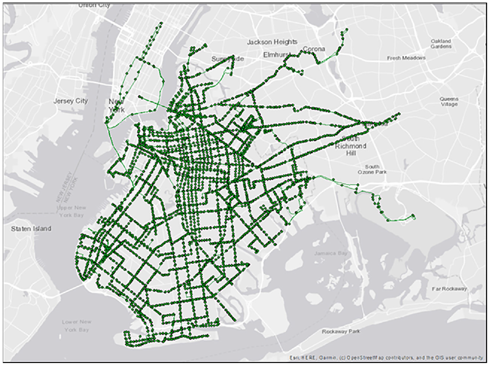
A synthetic population of NYC was created which incorporates the demographic information and travel patterns of 8.24 million people for the base year of 2016, as shown in Figure 1 ( 70 ). This results in 30,991,820 average daily trips made by the synthetic population. For this synthetic population, a tour-based nested logit model was estimated for Manhattan and non-Manhattan population segments ( 71 ).

Visualization of MATSim-NYC activities from synthetic population ( 70 ).
The modes Driving Alone, Carpool, Public Transit, Taxi, Bike, and Walk were estimated from the Regional Household Travel Survey. For-Hire Vehicles (FHV) and Citi Bike were calibrated to have cost and travel time coefficients similar to Taxi and Bike, respectively, with the alternative specific constants (ASCs) fitted to have the model outputs match the corresponding trip count data in 2016. Those modes were further estimated using the choice of a separately estimated smartphone ownership model as a feature for Citi Bike and as a condition for alternative availability for FHV. The validation of the model was conducted using the 2017 Citywide Mobility Survey provided by New York City Department of Transportation (DOT) and shown to be a good fit.
For the network topology, the base topology was converted into a network in MATSim from Open Street Map (OSM) and a transit network generated from General Transit Feed Specification (GTFS) data. For computation efficiency, the population in the simulation is scaled to 4% of the real population. By comparison, MATSim models in other cities like Berlin ( 72 ), Zurich ( 55 ), and Paris ( 65 ) use 10% scaled populations in their simulations. To avoid discretization errors (e.g., transit vehicles reaching capacity with just a handful of scaled agents, each representing 25 people), the transit line capacity was calibrated separately to 15% of original capacities which resulted in an average of 8% error with observed subway turnstile data ( 73 ). When it was set too low, the ridership would be diverted by the discretization, and when it was too high, it would not capture the congestion at the peak volumes. The green layer in Figure 2 shows the transit network. All transit vehicles run on dedicated links according to their schedules stored in the GTFS data, which is assumed to have been set under normal congestion conditions.
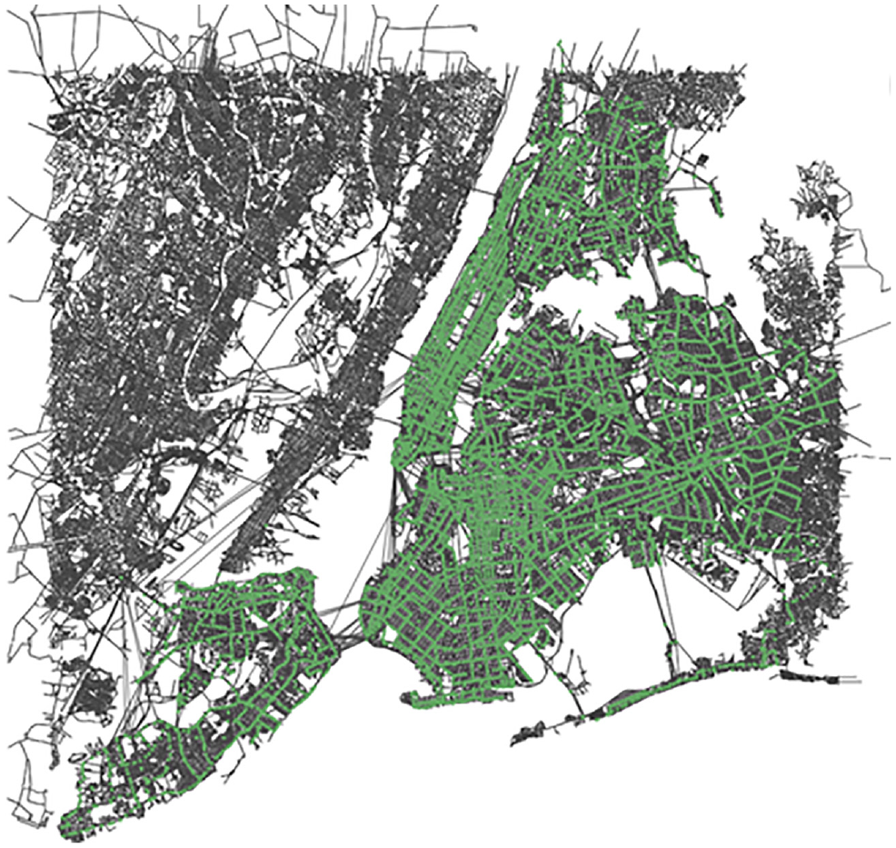
Transit (green) and road (gray) networks in MATSim-NYC ( 70 ).
INRIX data were used to calibrate unsaturated road speeds while the bridge-crossing average annual daily traffic (AADT) data were used to calibrate the road capacities. The validation of the MATSim-NYC trip assignment was conducted by comparing the outputs to two data sets: 10 stations from the 2016 Average Weekday Subway Ridership data and 15 traffic locations from the 2014–2018 Traffic Volume Counts data. The difference in daily ridership among the 10 stations is 8%, while the median difference in the traffic volumes among the traffic sites is 29%. Details of the calibration are in Chow et al. ( 70 ).
Methodology
Transit Route Frequency Design Model
Consider a network

Subject to


The objective function is to minimize the sum of each of the cost functions from Equation 2 defined as the route demand
The function is implemented with MATSim and calibrated (
The lower-level assignment is sensitive to the schedules set in the upper-level problem because MATSim captures travelers’ departure time elasticity; when departure time elasticity is combined with multiple mode choices, their elasticities are more realistically realized.
MATSim also captures such dynamic traffic propagation in the transit network as spillbacks in the flow, which are ignored in static trip-based models.
The multi-agent simulation simulates each individual separately, which results in a more realistic, heterogeneous population than a trip-based model.
Equation 2 is a line-level cost function. This means that the upper-level problem of optimizing the frequencies assumes that the demand in a network is already assigned to a transit line. This simplification is chosen to have a more tractable upper-level problem, relying instead on the lower-level MATSim model to resolve the assignment of passengers to the transit lines (i.e., this structure captures the interdependencies between the transit lines through the lower-level problem as a constraint to the upper-level problem).
As in Hasselström ( 25 ), a policy headway is used instead of a lower bound of 0 because the problem assumes a given set of routes in which transit frequencies are optimized. Allowing a lower bound of 0 implies that transit routes are being selected. In that latter case, the upper-level problem should also include route generation and a network-level cost function, leading to a different problem from the one solved in this study.
Like other transit NDPs in the literature, the model only deals with the strategic planning decisions of a line planning problem; it does not account for operational or tactical decisions like vehicle scheduling and crew scheduling.
Solution Method
The model is nonconvex; as such, our solution method is a heuristic designed to obtain a local optimum. An overview of the solution algorithm is shown in Figure 3. It is an adaptation of the Iterative Optimization Algorithm (IOA) from (
36
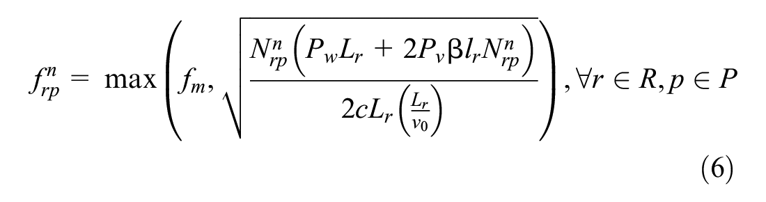
), where the upper level and lower level are iteratively updated with the solution from the other level. Given that the upper-level problem only has a minimum frequency constraint, the upper-level update can be determined for each route’s frequency independently by taking the derivative as shown in Equation 6. Since the bus stop delay is not modeled in MATSim,
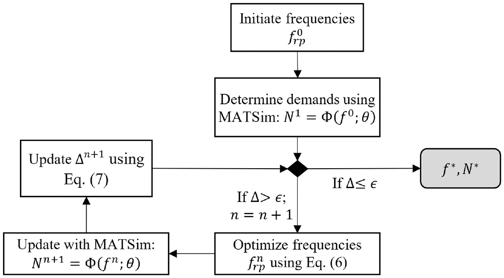
Flowchart for the proposed solution method.
The algorithm runs until a stopping condition is reached. In this case, the maximum difference in demand is used as the stopping condition

Case Study: Brooklyn Bus Network Redesign
Case Study Background
The existing bus network in Brooklyn, New York, is a large-scale system that dwarfs the transit services in some cities. It is composed of 78 bus routes and carries over 650,000 passengers per weekday ( 74 ). From the GTFS data, the network covers 550 route-km and has 4,696 bus stops. The minimum service frequency of each route at each hour per direction is constrained to two vehicles per hour to align with the MTA New York City Transit Service Guidelines ( 75 ). The trip demand pattern of the 4% population is visualized in Figure 4, where the blue line represents trips made with all modes, and the orange line represents trips made with the transit mode only. There are two distinct peak periods: 7:00 to 9 a.m. and 3:00 to 6:30 p.m. As the total number of trips increases, the number of transit trips increases but not directly proportionally. A trip-based model would treat each of these time periods as separate scenarios, but an activity-based scheduling model like MATSim would allow for adjustments in departure schedules throughout the day.
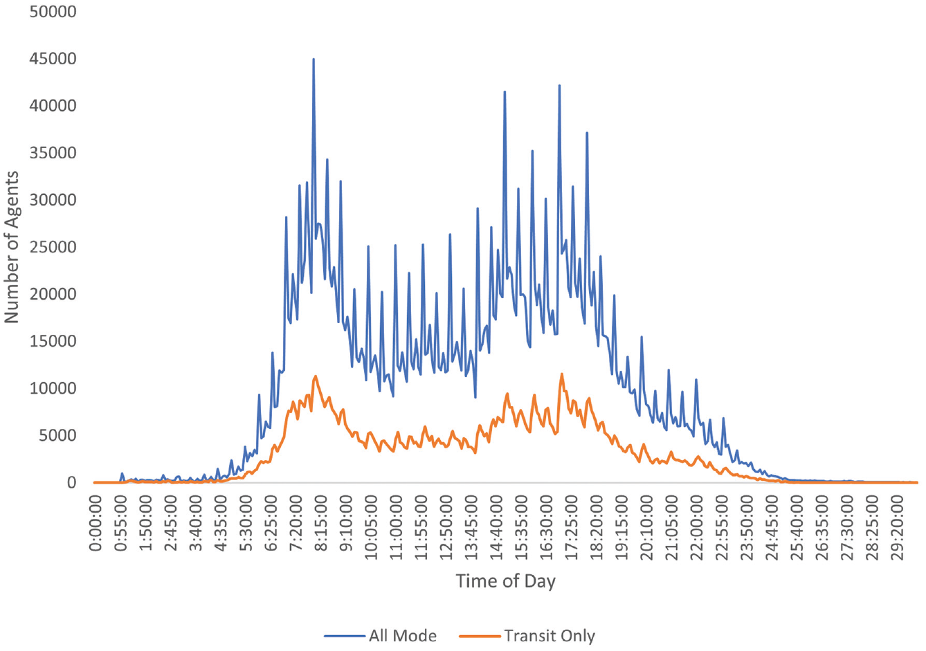
Time-of-day distribution of simulated trip demand in 4% population.
Drawing from lessons learned in the literature and the international community along with surveying 373 bus operators in Brooklyn, NYU Marron Institute’s Goldwyn and Levy ( 76 ) proposed a redesigned bus network shown in Figure 5 and presented in CityLab ( 77 ) and New York Magazine ( 78 ). The redesign increased stop spacing along with other technological improvements like all-door boarding and transit signal priority.
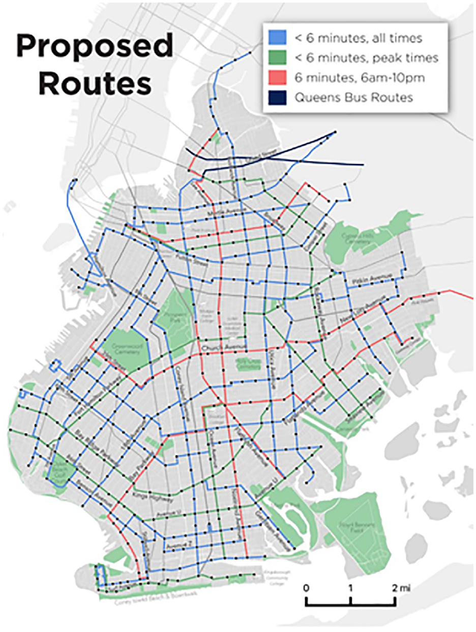
Brooklyn bus network redesign plan by Goldwyn and Levy (76)
The route plan includes stop locations and frequencies. How does it compare with the existing system? Can those frequencies be improved on? The study makes comparisons between three scenarios:
Scenario 1: Existing Brooklyn bus network (with volumes calibrated to average ridership levels provided by MTA)
Scenario 2: Goldwyn and Levy’s proposed bus network redesign with their specified frequencies
Scenario 3: Goldwyn and Levy’s proposed bus network redesign, with the optimized frequencies using our proposed model.
For Scenarios 2 and 3, there is no GTFS data, so a GTFS schedule was created for each. For Scenario 3, the frequency optimization algorithm specified was used to design frequencies. These are then used to compare with Scenario 2.
All the data for the case study can be accessed at https://doi.org/10.5281/zenodo.3894549.
To evaluate how well any of the scenarios work, the performance measures of these designs are obtained using MATSim-NYC ( 70 ) presented above. The calibrated model incorporates eight modes: drive alone, carpool, transit, taxi, walk, bike, ride-hail, and bike-share. By evaluating these mode choices within a dynamic scheduling setting, it considers the substitution of modes alongside departure time choice, which fits the needs of a transit timetable design problem. Running the frequency optimization with the calibrated MATSim-NYC takes the competition with other modes into account.
Scenario Testing
The first scenario tests the existing bus operation. January 2020 MTA GTFS is imported to MATSim-NYC and tested to establish a baseline. The output is analyzed in detail and compared with the published ridership. The simulated ridership is scaled to match the published ridership, and this scaling factor is kept the same for the rest of the scenarios.
Lam and Small ( 79 ) report that the value of time at Orange County, California is $22.87. Since the cost of living in Orange County is comparable to New York City, we decided to test Scenario 3 with an in-vehicle travel time of $20/hr and a wait time cost of $35/hr, based on more than 50% wait time premium in Balcombe et al. ( 80 ). Table 1 lists the global parameters used in the simulation, where
Testing Parameters for All Scenarios

Note: vph = vehicles per hour.
c is the operation cost for buses, and
A minimum frequency of 2 h is used and the day is divided into 24 hourly periods.
Proposed Transit Network Configuration
When evaluating the new scenarios, the Brooklyn bus network shown in Figure 6 is cut out and replaced with the proposed networks.
Existing Brooklyn bus network.
For Scenarios 2 and 3, we refer to Goldwyn and Levy’s ( 76 ) proposed bus network redesign. The network is visualized in Figure 7a. Major attractions are marked with red triangles; bus depots are marked with a green bus sign. Compared with the existing average operation speed of 7.2 mph for Brooklyn buses ( 81 ), Levy and Goldwyn propose to speed up the buses to 9.32 mph (15 km/h) by implementing off-board fare collection, stop consolidation, dedicated lanes, and signal priority. To provide sufficient frequency, they also propose to consolidate the network from the current 550 km to about 355 km. The network is then converted into XML, and is visualized on Simunto Via (a MATSim visualization software), shown in Figure 7b. Because Scenario 2 differs from Scenario 1 by more than just network design considerations but also other interventions, it should be clear that Scenario 1 does not represent a “network design benchmark” but rather provides a contextual background to compare Scenario 3’s performance with that of Scenario 2.
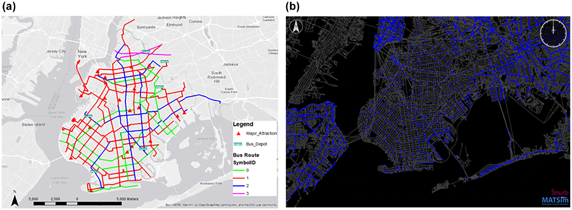
Goldwyn and Levy’s ( 76 ) bus redesign: (a) on a Geographic Information System (GIS); and (b) imported into MATSim.
Results
MATSim-NYC is run to 100 days of iterations to adjust passenger demand to the scenario design, which means that each run in the optimization algorithm would go through 100 days (by comparison, MATSim’s Munich model produces a similar travel time distribution using 5% of agents in 50 days compared with 100% of agents in 500 days; the overall computation time is 50 times faster) ( 82 ). Additionally, running 100 days of iterations ensures that every agent in the simulation has at least one chance to re-plan their activity and mode. One run requires about 11 h on a PC with an Intel Xeon E5-2637 CPU and 128 GB RAM. In practice, we recommend that users reserve at least 70GB of RAM to run our 4% MATSim-NYC model. The computation time is relatively high because of the large number of agents and NYC’s complex network.
To compare the city level performance, Figure 8, a to c, show the mode statistics and score statistics of all the agents in the simulation (of the final iteration of the network design). The jump at the 80 iteration is because re-planning was turned off, given that each agent in the simulation had at least one opportunity to re-plan their activity and travel mode. The remaining 20 iterations are then used to resolve the final plans’ performances.
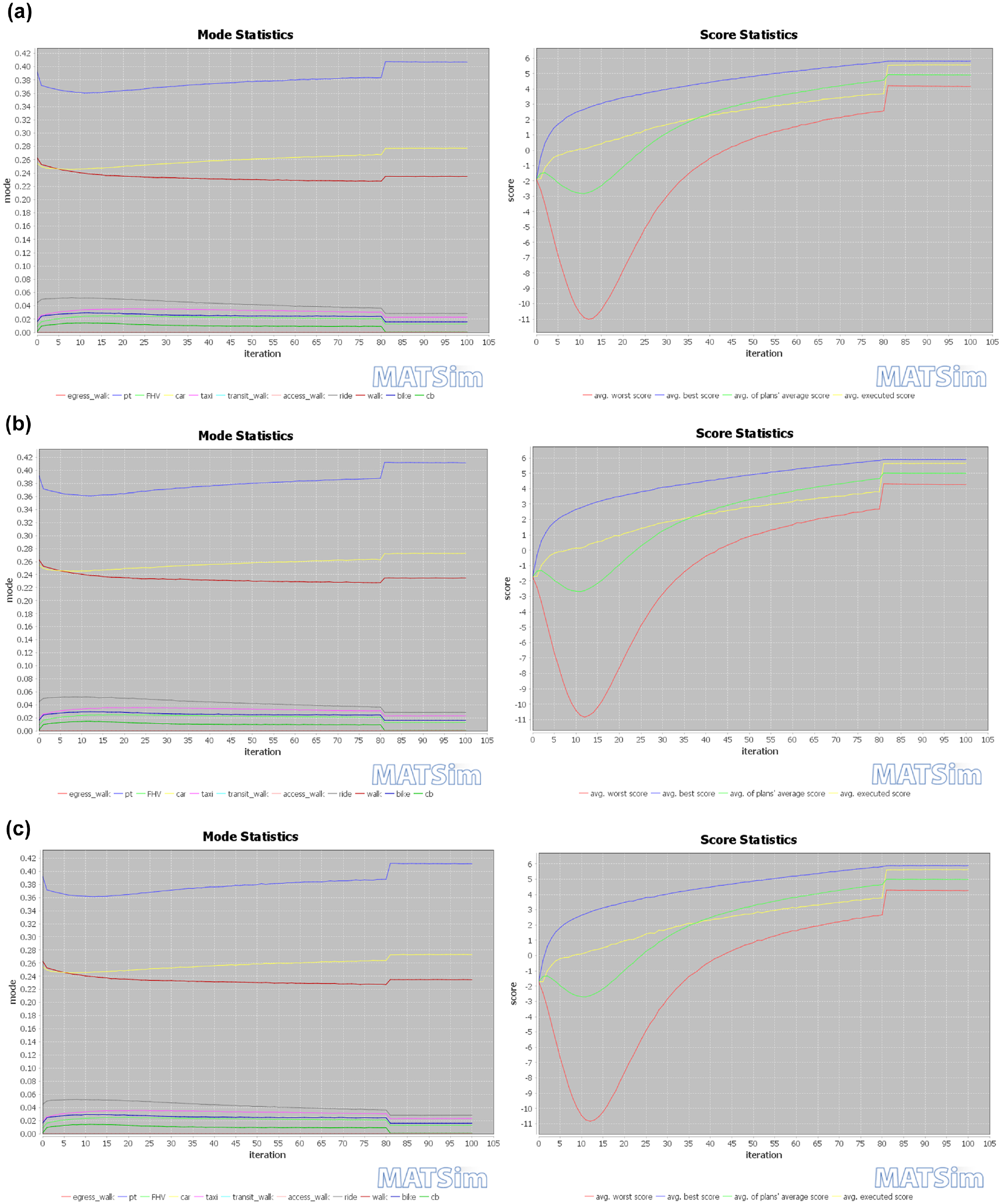
MATSim simulation statistics for: (a) Scenario 1; (b) Scenario 2; and (c) Scenario 3.
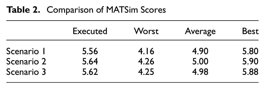
Table 2 includes the executed, worst, average, and best MATSim scores for all three scenarios. In the city level, the MATSim score increased by an average of 2.04% and 1.63% for Scenario 2 and Scenario 3 compared with Scenario 1. An increase in the MATSim score in these two scenarios signals that the whole population in New York City is likely to be better off after the introduction of the redesigned Brooklyn bus network.
Comparison of MATSim Scores
Scenario 1 Calibration Results
The existing transit network is run in MATSim-NYC for one run and the results are compared with existing MTA ridership numbers. Because MATSim-NYC was calibrated overall at the citywide level considering both subway and bus for one transit mode, there are discrepancies to the total Brooklyn bus ridership values. Assuming the distribution of ridership is adequate, we add a further calibration factor for the Brooklyn bus network by applying a scale factor to the ridership to make it match the total Brooklyn bus ridership. A factor of 3.69 was applied to the output MATSim-NYC bus ridership to scale it to the observed ridership.
The resulting scaled MATSim-NYC ridership is compared at the line level to the observed ridership in Figure 9. The average of the relative differences is shown to be 30% while the median difference is 17% (this means there are a few large outliers). None of them have an observed ridership greater than 10,000 daily trips. When weighted by ridership, the ridership-average difference across the routes is 21%. This suggests the distribution of the ridership is within a reasonable range (see Flyvbjerg et al. [ 83 ]).

Route level ridership error.
Algorithm Convergence for Scenario 3
Having calibrated for Scenario 1, we proceed to solve for the frequencies using the proposed algorithm in Scenario 3. Since the proposed network redesign has 39 routes (setting different frequency for each direction separately resulting in 78 effective routes), we optimize them over 24 hourly periods, resulting in 1,872 frequency decision variables and 1,872 route-demand variables aggregated from MATSim each iteration, for a total of 3,744 decision variables.
The initial guess frequencies are six trips per hour per route per direction during extended peak hours (5 to 10 a.m. and 4 to 9 p.m.), and two trips per hour per route per direction during off-peak hours (midnight to 4 a.m., 11 a.m. to 3 p.m., and 10 to 11 p.m.). Ten iterations of the proposed algorithm were run to find a stable solution. Figure 10 shows the trajectory of the algorithm for Scenario 3 in ridership and number of bus trips. The number of riders increases monotonically each iteration until iteration 5, after which the algorithm stabilizes with
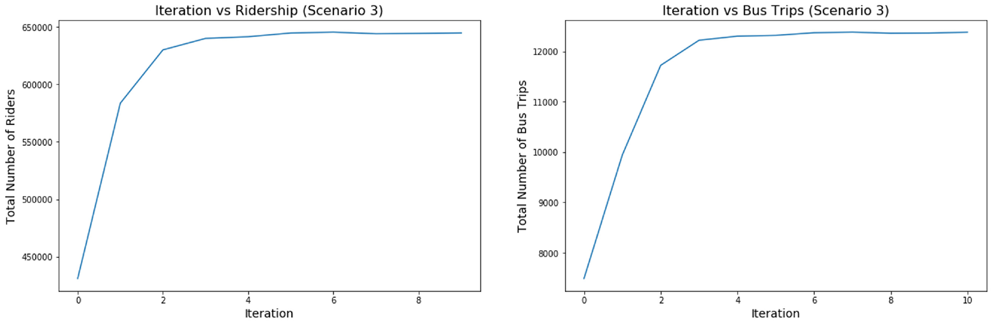
Ridership and vehicle trips trajectories for the proposed algorithm used in Scenario 3.
Scenario 3 Output Summary
Based on the experienced plans from each agent in the simulation, we can aggregate the number of riders who depart from or arrive at each transit stop station per day. Figure 11 shows the stop boardings and alightings for Scenario 3, where the red bars represent the aggregated number of agents who depart from a station, and the green bars represent the aggregated number of agents who arrive at a station.
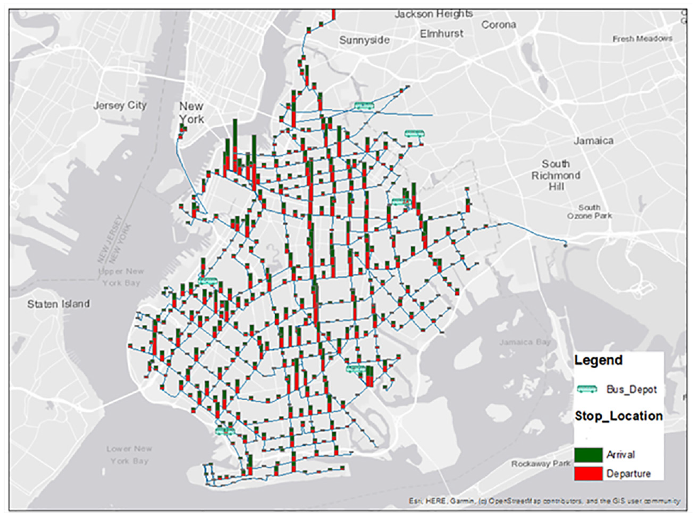
Bus stop boardings and alightings.
From our simulation, we can aggregate the number of vehicle trips provided each hour, which reflects the output frequencies for the routes in the network. Figure 12 shows the vehicle trips provided for each hour by stacking the frequency of each route at different hours of a day. The left part of the figure is based on Goldwyn and Levy’s ( 76 ) headway design, and the right part of the figure is the simulation output for Scenario 3. Scenario 3 provides a significantly lower number of vehicle trips at midday and evening. Engineers and planners can use these figures to guide their timetable, vehicle scheduling, and crew scheduling designs.
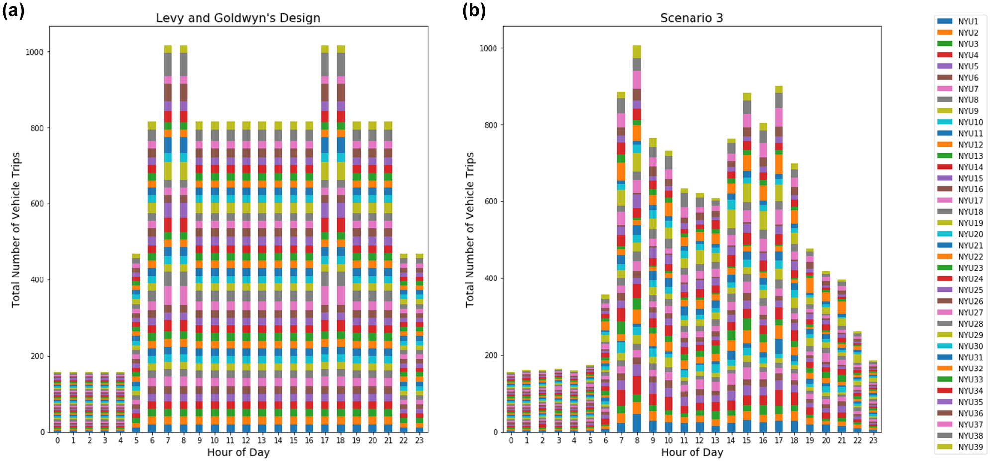
Trips provided per hour for the proposed design for Scenarios 2 and 3.
Ridership Comparison
The daily riderships across the three scenarios are summarized in Figure 13, a to c. They show that the existing ridership is relatively low per length of bus route, but by redesigning the routes and frequencies, it is possible to attain higher ridership throughout. Scenario 3 optimizes the frequency of each route. The main difference between Scenarios 2 and 3 is the midday and late evening hours, when Scenario 3 provides a significantly lower number of trips. Qualitatively, comparing Figures 4 and 12, the solution in Scenario 3 matches the trip demand profile better because of using an activity-based scheduling model that captures time-of-day responses.
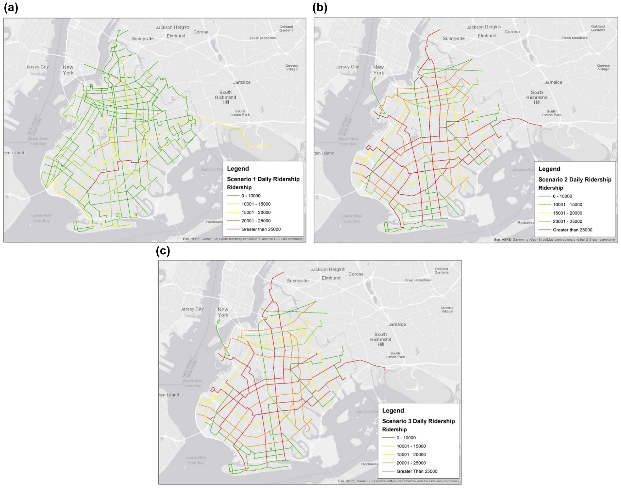
Comparison of daily ridership for: (a) Scenario 1; (b) Scenario 2; and (c) Scenario.
A detailed comparison between specific routes can be made. For example, the load profile for different routes can be extracted from the simulation. This is done for the northbound Nostrand/Lee/Bedford route from 8 to 9 a.m. for both Scenarios 2 and 3 in Figure 14, a and b, respectively. They indicate that the frequency change between designs results in a noticeable change in user demand, such as the increase in ridership in the segment between 4 and 4.8 mi on the route for Scenario 3 corresponding to the Newkirk/Rogers, Beverly/Rogers, and Rogers/Church stops.
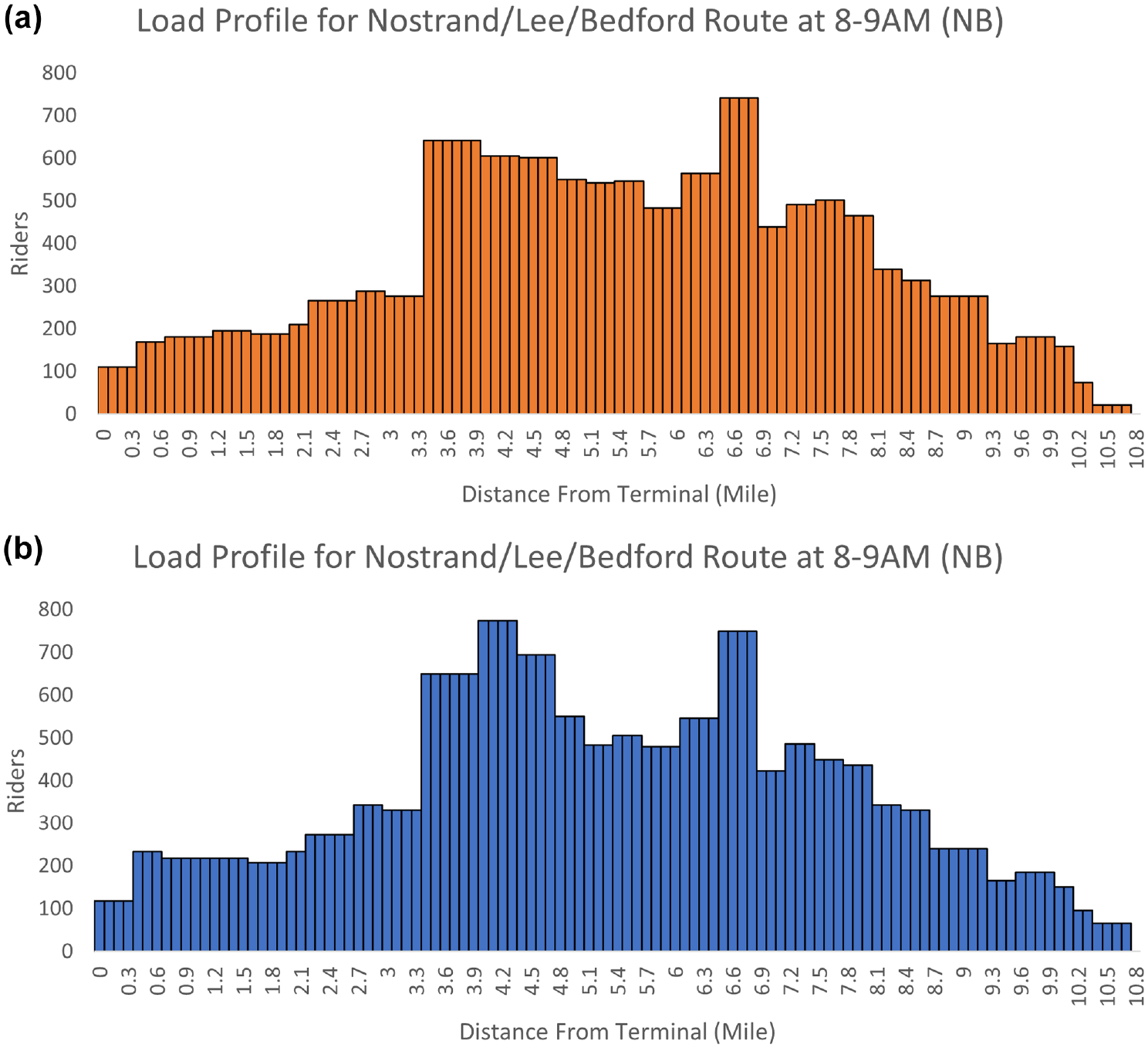
Comparison of 8 to 9 a.m. load profiles for the northbound Nostrand/Lee/Bedford route in: (a) Scenario 2; and (b) Scenario 3.
Farebox Recovery Ratios
The three scenarios are compared for operating cost, ridership, fares collected, and farebox recovery ratio, as shown in Table 3. The operating costs are based on the same parameters used for determining the operating cost shown in Table 1, used to compute the cost for each network of routes according to their frequencies. The revenue is based on the simulated ridership for all three scenarios in MATSim. This ridership reflects the costs of transit to the riders who use the system. Increased wait times (because of lower frequencies) or in-vehicle times would result in changes in ridership.
Comparison of Simulated Daily Metrics Between Scenarios

The results suggest that the bus network redesign from Goldwyn and Levy ( 76 ) would increase demand by 23% while reducing operating cost by 6%. This result is also similar to their estimated ridership increase of 20%. Meanwhile, the proposed frequency setting leads to a more balanced outcome: ridership improves over the existing level by 20% but also reduces operating costs by 25%. This is a small 3 percentage point drop from the Goldwyn and Levy ( 76 ) design with an accompanying 19 percentage point reduction in operating cost.
Although the basic fare is $2.75, many riders have discounts or free rides through various programs for seniors, students, monthly passes, and so forth. To account for this, we determine an equivalent fare per passenger to calibrate to the observed farebox recovery ratio from the MTA (74) of 0.22. The resulting equivalent fare is $1.14, which we apply to the other scenarios. Goldwyn and Levy’s ( 76 ) design increases the farebox recovery ratio by 30% to 0.29 by providing faster and more frequent services. Scenario 3 provides a more balanced solution, whose vehicle miles traveled per day is similar to the existing MTA system, but can attract more customers. It is more efficient compared with Goldwyn and Levy ( 76 ) because many of the unnecessary trips during midday and evening are taken away based on the demand. The farebox recovery ratio for Scenario 3 is 0.35, which is a 60% improvement over Scenario 1.
Mode Substitution
Because the simulation outputs individual agent choices, we can determine where all the new ridership is coming from in Scenarios 2 and 3. This helps answer the question of how redesigning the bus network in the presence of ride-hail services as well as other modes would affect travelers’ likelihood of choosing the bus. The results are shown in Figure 15. In both scenarios, the major mode drawn from is by car (74%), which is a very encouraging result. Only 2.5% to 2.6% (this amounts to about 2,700 daily trips by ride-hail) of the new trips in the bus redesigns would come from ride-hail, which suggests there is not so much competition between the two modes. Nearly 12% of new trips would be drawn from walking, which suggests that the redesign is able to provide a more convenient alternative to people who otherwise would have walked only.
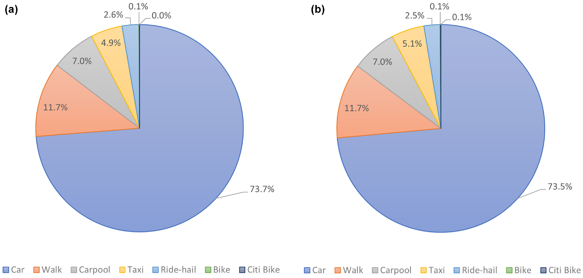
Modes shifted to new bus ridership in: (a) Scenario 2; and (b) Scenario 3.
Conclusion
In sum, this project has two main contributions. First, we proposed a simulation-based transit network design model for bus frequency planning in large-scale transportation networks with activity-based behavioral responses. The model is applied to evaluate the existing Brooklyn bus network, the proposed network redesign in Goldwyn and Levy ( 76 ), and propose an alternative design based on our methodology.
The MATSim-NYC model from Chow et al. ( 70 ) is generally able to simulate patterns similar to the existing bus network in Brooklyn with some calibration. A line-level comparison to observed ridership shows a ridership-weighted average of 21% difference between observed and simulated route ridership, with a few outliers for the smaller volume routes.
An iterative simulation-based frequency bilevel optimization model is proposed that uses an analytical model to set frequencies and a simulation model (MATSim-NYC) to update demand. Numerical tests show that the algorithm converged to an equilibrium outcome.
Comparisons of the Goldwyn and Levy ( 76 ) design with the existing scenario confirms their claim that their design can increase ridership by 20% (our simulation result suggests an increase of 23%), at a reduction in operating cost of 6%. By using our simulation-based frequency setting approach, however, we can further improve operating cost (to 25% reduction from Scenario 1) while maintaining a 20% increase in ridership from Scenario 1. As a result, our simulation-based optimization approach can improve on network redesign in Goldwyn and Levy ( 76 ) to increase the farebox recovery ratio from an improvement of 30% up to 60% over the existing scenario. The increased ridership draws primarily from passenger car use (nearly 75%), with a small 2.5% drawn from ride-hail services and another 5% from taxis. This suggests the redesigns should be effective in moving people away from less efficient transportation modes.
Future research will look at operationalizing the process of designing transit networks using the simulation-based approach combined with line-level cost functions as a tool for policymakers. For alternative transit NDPs that consider route generation, transit network-level cost functions will be considered as well. The perspectives of multiple operators (e.g., Pantelidis et al. [ 84 ]) could also be considered in future studies to find design solutions that are amenable to multiple parties, particularly for MaaS settings. More efficient algorithms, such as surrogate-based optimization (e.g., Chow et al. [ 19 ], Zhou and Chow [ 85 ]), can be explored to overcome computation costs.
Footnotes
Acknowledgements
The proposed Brooklyn bus redesigned plan was shared by Dr. Eric Goldwyn, who is greatly appreciated.
Author Contributions
The authors confirm contribution to the paper as follows: study conception and design: Z. Ma, J. Y. J. Chow; data collection: Z. Ma; analysis and interpretation of results: Z. Ma, J. Y. J. Chow; draft manuscript preparation: Z. Ma, J. Y. J. Chow. All authors reviewed the results and approved the final version of the manuscript.
Declaration of Conflicting Interests
The author(s) declared no potential conflicts of interest with respect to the research, authorship, and/or publication of this article.
Funding
The author(s) disclosed receipt of the following financial support for the research, authorship, and/or publication of this article: This research was conducted with support from the C2SMART University Transportation Center (USDOT #69A3551747124) and the FHWA Dwight David Eisenhower Fellowship program.
All the errors and views expressed in this study are those of the authors.