Proposal for a Pivot-Based Vehicle Trajectory Clustering Method

Abstract

Given the large volume of georeferenced information generated and stored by many types of devices, the study and improvement of techniques capable of operating with these data is an area of great interest. The analysis of vehicular trajectories with the aim of forming clusters and identifying emerging patterns is very useful for characterizing and analyzing transportation flows in cities. This paper presents a new trajectory clustering method capable of identifying clusters of vehicular sub-trajectories in various sectors of a city. The proposed method is based on the use of an auxiliary structure to determine the correct location of the centroid of each group or set of sub-trajectories along the adaptive process. The proposed method was applied on three real databases, as well as being compared with other relevant methods, achieving satisfactory results and showing good cluster quality according to the Silhouette index.

Keywords

data and data science artificial intelligence and advanced computing applications machine learning (artificial intelligence)pattern recognition geographic information science GPS data

Technological advances have made it easy for devices to record information in various scenarios, giving rise to large volumes of data in very diverse formats. This has increased interest in techniques capable of analyzing such data to identify the most relevant features and to recognize relationships or emerging patterns that help decision making. For example, Kang et al. ( 1 ) developed an algorithm to extract significant places visited by individuals from a trace of coordinates originated from WiFi access points. In a different context, Li et al. ( 2 ) explored the similarity between users based on spatio-temporal location histories, using GPS data collected by 65 volunteers over a period of 6 months.

On many occasions, information arising from geographic positions could help in the definition of public policies related to urban growth or public services. In this context, the analysis of spatial data generated by the various location technologies used today is of vital importance for the elaboration of urban development plans for cities. Large volumes of these spatial data, produced by Geographic Information Systems (GIS), are used by governments in urban planning, transportation engineering, territorial analysis, and other areas ( 3 ). Within these systems, the spatial component is implemented with a specific geographic location.

Having strategies to identify common features in spatial data (geographic locations) has proven useful in different urban planning applications. For example, through the characterization of people’s mobility profiles, urban planning related to the management of recreational facilities can be improved. Additionally, this information could be used, for example, to plan commercial activities, promote car sharing systems, and, among other things, to evaluate driver behaviors as observed in this paper ( 4 ).

It is often also necessary to know the characteristics of regions or places and the moblity characteristics of entities. For example, to identify the most common origins and destinations or when these entities move in large numbers and where they stop. These two problems translate, respectively, into applications capable of characterizing regions (mainly the discovery of hot spots) and moving objects (mainly determining the mobility of people or other entities) ( 5 ).

Transportation systems also influence urban planning and development, since identifying congestion areas in a city, and the analysis of these areas, is vital to the future construction of transportation infrastructure or road corridors that improve mobility. In addition, developments in the transport sector demand increasingly efficient techniques for the analysis of spatial data.

Intelligent Transportation Systems (ITS) process large amounts of trajectory data generated from vehicles on the roads in real time (6–9). A trajectory is defined by a set of geographic locations, each of which is represented by its latitude and longitude, at a moment in time. Intelligent trajectory analysis can assist in assessing road performance regardless of the type of road (streets, highways, etc.), as evidenced in ( 10 ), which proposes a new methodology for solving the optimal roadway segment configuration problem.

The ITS has methods to perform traffic flow analysis in specific sectors of the city. These methods can be enhanced using additional information from the same system, for example the direction of the trajectory, the average speed of a group of vehicles in an specific time or the number of vehicles in a spatial-temporal location. This additional information can help to predict futures traffic jams, accidents, low traffic flow in some areas between other things, providing information to decision makeres, as evidenced in (11, 12), which discuss a clustering approach to assessing travel time variability. By contrast, ( 13 ) analyzes hot spots based on regions. One of the methods used in traffic analysis is segmentation ( 14 ). To facilitate this analysis a clustering method must be used. There are several methods in the bibliography with advantages and disadvantages but variables like precision and the quality of vehicular concentration groups can be improved.

In this research we analyze various clustering methods to compare the strategies used to create the groups and the similarity measures used to get the majority of the information. We present a novel clustering technique based on a pivot concept to enhance the quality of the groups in the clustering process. The proposal allows analysis of the clustering of trajectories within several sectors of a city. This analysis is useful when applied to road planning and can be enriched by considering other moving objects within a city.

The aim of this paper is to propose an alternative clustering method. This method is based on pivots and performs partitive clustering of vehicle trajectories, departing from the well-known K-means method (15, 16). The algorithm generates clusters given by the average trajectories (i.e., centroids) of each group. In this sense, the use of pivots is a fundamental tool for correctly identifying the closest group for each sub-trajectory. This directly affects the dispersion of elements within each group, as will be explained in the discussion of the results.

The method proposed in this article may be useful for traffic managers planning urban roads, reducing congestion levels, detecting hotspots, improving traffic flow, identifying anomalous traffic situations, and predicting future behaviors ( 17 ). Furthermore, better traffic flow management leads to environmental improvements. The algorithm was applied to three data sets with real, non-simulated data to guarantee the empirical validity of its performance.

This paper contributes to the existing literature in several ways: i) it proposes a trajectory segmentation phase based on the angles formed between two trajectory locations. The partitioning and generation of sub-trajectories depend on a threshold angular value; ii) it adds a mechanism for the selection of initial centroids with the definition of a lattice in the area to be analyzed; and iii) it proposes a trajectory clustering method that uses novel centroid recalculation by means of pivots.

The remainder of the paper is organized as follows: the first section discusses the related literature and presents alternative solutions to the problem under examination; we then describe the proposed trajectory clustering method using the pivot; this is followed by a description of the data used in the experiments; we then present and discuss the results obtained in the three data sets; finally, we draw conclusions and discuss possble future research lines.

Literature Review

Techniques used to analyze data are divided into two broad groups: those that operate on labeled information and those that do not. The first group corresponds to predictive models, while the second generates descriptive models. A predictive model offers a response to a new situation and is generated from the observation and generalization of the responses given in previous situations. In other words, to obtain one, it is necessary to know the answer or label from many previous cases. Descriptive models seek to identify similarities between the recorded data to identify situations or behaviors within a process without requiring prior labels. The analysis of trajectories presented in this paper belongs to the second type. The objective is to recognize similarities in the trajectories, considering not only the geographic locations involved but also other aspects related to specific situations, such as density changes. Such changes occur in congestion or under anomalous traffic patterns and are extremely useful for predicting accidents.

There are different techniques to build descriptive models, grouping or clustering being the most widely used ( 18 ). Currently, clustering techniques identify groups of instances with similar characteristics from which patterns or relationships can be extracted. They can be adapted to very diverse fields such as health, finance, telecommunications, agriculture, and transportation, among others ( 19 ).

Several researchers have attempted to address the limitations identified in certain techniques, such as Varghese et al. ( 3 ). Other researchers have modified existing techniques to apply them to specific contexts, such as spatial data mining (20, 21) and the analysis of trajectories ( 5 ).

The analysis of trajectories involves large volumes of data, which are usually processed incrementally, that is, as the data are recorded. This type of processing requires certain special considerations. An incremental clustering technique is proposed by Li et al. ( 22 ). It seeks to respond to this type of situation based on a strategy defined by Aggarwal et al. ( 23 ) to cluster data flows.

In the literature related to clustering techniques in the transport area, there are some contributions oriented to the analysis of transport flows in cities to improve urban planning (24, 25), while others are aimed at clustering trajectories ( 26 ). Some other papers discuss the clustering of trajectories in a road network environment. This problem can be solved by the combination of map matching and graph clustering algorithms. Other lines of research discuss methods for trajectories in free spaces ( 27 ).

Trajectory Clustering Algorithms

Classical clustering algorithms deal with vector data of fixed dimensions. Unlike these classical algorithms, trajectory clustering algorithms process information with different characteristics such as temporal sequential information and in some cases the length of these trajectory data is different within the same data set.

Gaffney and Smyth ( 28 ), using a probabilistic regression model, gave rise to one of the first density and distance-based approaches to trajectory clustering, these early clustering approaches used in analysis of trajectories make use of partitive and density-based algorithms ( 29 ). Partitive clustering algorithms gather observations or examples into several pre-specified clusters. These algorithms start from a random partition that is then refined by iterations, that is, moving an object from one cluster to another. K-means ( 16 ) is an example of this type of algorithm. Nanni ( 30 ) made an adaptation to make these algorithms capable of processing trajectories by using two classical distance-based clustering algorithms (the classical K-means algorithm and the hierarchical agglomerative method). Density-based algorithms start the cluster from one object, and the cluster grows as long as there are new objects in the neighborhood. The cluster is considered valid if the total number of objects exceeds a threshold. DBScan is a member of this algorithm family ( 31 ). Several papers adapt existing algorithms to a particular context using unconventional measures of similarity between trajectories (32–34). The Enhanced DBScan algorithm ( 35 ) improves on the traditional DBScan algorithm (36, 37) using its own density measurement method (movement capability), which relies on adjacent points along the trajectory. Additionally, it combines two consecutive stops with the same geographic location and a short time interval, using the method developed by Yuan and Raubal ( 34 ). The Tra-DBScan algorithm ( 38 ), based on the DBScan algorithm ( 31 ), adds a trajectory segmentation phase and partitions the trajectories into sections using the Hausdorff distance as the similarity measure. This metric considers the perpendicular, angular, and parallel distances of the different GPS points that are part of the trajectory segments. Ferreira et al. ( 39 ) introduce a new trajectory clustering technique that uses vector fields to represent the centers of the clusters and propose a definition of similarity between trajectories. The K-means vector field, while reminiscent of the K-means algorithm (40, 41), is a new formulation for trajectory clustering, with the ability to find global patterns that are not locally apparent in noisy trajectories or even partial trajectories. Additionally, the algorithm can be paralleled, allowing escalation into large data sets. Yu et al. ( 42 ) propose an improved trajectory model and present a new clustering algorithm that uses a measure of similarity based on multiple characteristics of the trajectories, thus maximizing their value when it comes to elements of the same group. Recently, Yang et al. ( 43 ) proposed a new trajectory clustering algorithm called TAD. Some of its main advantages are as follows i) it introduces a noise tolerance factor, which can dynamically evaluate and reduce the impact of noise in the algorithm execution process; ii) it integrates time and space features into a single measurement function to improve grouping accuracy; and iii) it builds a new density function, which accurately distinguishes different types of points in trajectories and finds trajectory stays based on space-time density data analysis. This algorithm also defines two new metrics: Motion Capability and Neighborhood Time (NMAST) and Noise Tolerance (NT). Another approach is based on segmentations or partitioning and proposes dividing the trajectories into segments before grouping them. Dividing them into segments makes it possible to analyze areas in a more specific way by identifying different places crossed by various trajectories (5, 44). TRACLUS clustering algorithm uses this second approach ( 45 ). Ailin et al. ( 46 ) also use the segmentation of trajectories at a specific time, making use of this technique to partition the trajectories according to the threshold given by the Minimum Description Length (MDL) principle and then employ a Density Peak Clustering (DPC) process which allows them to extract the trend of the trajectories’ movements. Zhou et al. ( 29 ) propose a clustering method that uses trajectory regressions and angle-based partitions to avoid getting stuck in local optima. The following papers have been identified among others also based on this approach (47–49). Another approach is to analyze road networks in conjunction with trajectories, Hong et al. ( 50 ) propose an algorithm that employs similar spatio-temporal clustering, which takes into consideration the topological relationships that make road networks. Yu ( 51 ) proposes a multilevel method in which network analysis and association rules are put together to efficiently obtain the movement patterns of trajectories. Feng et al. ( 52 ) take into account a static topology of road networks to create a directed weighted complex network, in which spatio-temporal changes over critical roads and intersections are identified. Niu et al. ( 53 ) also perform a similar approach using a road network through a dual graph model to identify the similarity between the nodes used. The development of these algorithms has given rise to new approaches that specialize mainly in making trajectory predictions using space-time techniques to consider the dynamic evolution of trajectories ( 54 ) used on large-scale data. Wang et al. ( 55 ) use the above scheme as a base and add the use of artificial intelligence models to classify the data and demonstrate the search potential on the resulting clusters. Tallapragada and Cortes ( 56 ) on the other hand, consider the coordination of traffic at intersections and determine clusters as they appear, trying to optimize the results for individual trajectories. To consider the dynamic nature of the data, some of this approach makes use of the characteristics of the created clusters themselves, as in the case of Huang et al. ( 57 ), who make use of additional information such as stopping and waiting times of vehicles to provide solutions to alleviate traffic at certain times. Tang et al. ( 58 ) analyze urban trajectories using a fusion of spatial, temporal, and directional attributes to provide traffic planning and management strategies. Kumar et al. ( 59 ) have focused on solving a problem that arises as these approaches evolve, which is the handling of a large-scale spatio-temporal data volume, proposing new more efficient distance measures and an algorithm to determine the number of optimal clusters, this could be applicable in those using data mining techniques obtained from big data, which will affect the performance of the algorithm employed as they will require more processing power to be viable; other alternatives use Markov chains ( 60 ) or R-trees ( 61 ) to create index structures that reduce the employed cost of time. Liu and Zhang ( 62 ) emphasize the importance of distance calculations to reveal differences between trajectories and promote higher accuracy of algorithms by adaptive selection of clusters and their characteristic features.

A full review of the object trajectory clustering algorithms exceeds the scope of this paper. We, therefore, refer to a recent review that surveys and summarizes recent trends on moving object clustering algorithms ( 63 ).

Trajectory Similarity Metrics

There are different clustering techniques for analyzing trajectory data. On the one hand, some use traditional similarity or distance metrics (e.g., Euclidean distance, Manhattan distance, etc.) to identify a trajectory and assign it to a specific cluster (64, 65). On the other, there are techniques that use non-traditional similarity metrics (66, 67).

An additional line of research proposes the use of a deep neural network (DNN) to develop a supervised similarity model ( 68 ). The similarity metrics considered in the literature include: distances limited by the network, distances based on form, and distances based on warping (66, 67). Network-limited distances use the underlying road network, and assume that the road network is known and that the trajectory data are perfectly mapped on it. Shape-based distances seek to identify the geometric characteristics of trajectories by emphasizing their shape. Distances based on warping take the temporal dimension into account.

Proposed Method: Trajectory Clustering Using Pivots

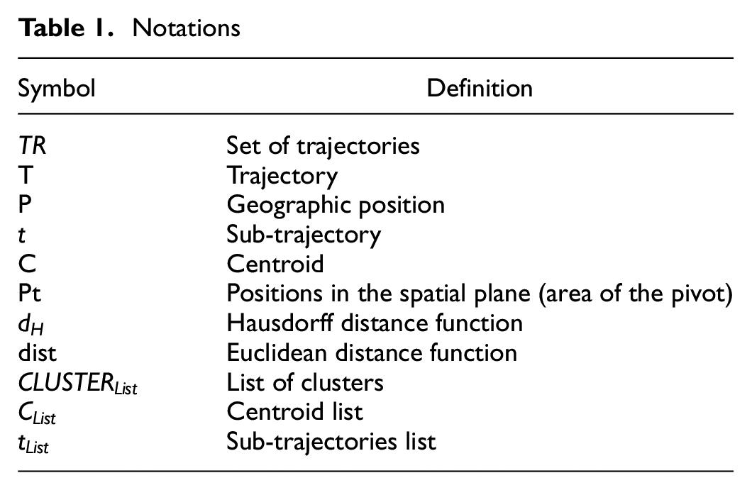
The present proposal uses the trajectory segmentation strategy introduced by Reyes et al. ( 44 ) and incorporates a pivot as a device to calculate the average trajectories (i.e., centroids) of each group. Thus, the proposed method is called K-pivot. An important aspect of any clustering method is the correct initialization of the centroids. In this paper, we propose setting a grid that encompasses all trajectories. Table 1 shows the notations used in this paper.

Table 1.

Notations

Symbol	Definition
$TR$	Set of trajectories
T	Trajectory
P	Geographic position
$t$	Sub-trajectory
C	Centroid
Pt	Positions in the spatial plane (area of the pivot)
$d_{H}$	Hausdorff distance function
dist	Euclidean distance function
$CLUSTE R_{List}$	List of clusters
$C_{List}$	Centroid list
$t_{List}$	Sub-trajectories list

A trajectory is defined as a sequence of geographic positions, each represented by its latitude and longitude. In other words, the $i -$ th trajectory can be written as $T R_{i} = (P_{1}, P_{2}, \dots, P_{s})$ , where each position $P_{s}$ is a vector with form $P_{s} = (longitude, latitude)$ . A sub-trajectory $t$ is a portion of a trajectory $TR$ conformed by a sequence of geographic positions belonging to a trajectory $T R_{i}$ and is defined as $t = (P_{i}, P_{i + 1} \dots P_{j})$ where $(1 \leq i < j \leq s)$ .

A cluster is a set of sub-trajectories. A centroid is a sequence of geographic positions that represents or characterizes all the sub-trajectories of a cluster and can be written as $C_{List} = (C_{1}, C_{2} \dots C_{k})$ where $C_{m} = (longitude, latitude)$ with $(1 \leq m \leq k)$ .

A pivot in this paper is defined as a line segment in the area where a majority of the sub-trajectories of a cluster are located. To obtain the direction of the pivot, the angles of each sub-trajectory with respect to the coordinate axis are averaged. The number of positions in the pivot coincides with the average number of positions that make up the sub-trajectories of the corresponding cluster. The pivot is a guide to the centroid recalculation process.

The trajectory clustering method consists of the following phases:

Segmentation

Grid setting

Clustering.

In the segmentation phase, the trajectory is divided into segments or portions called sub-trajectories. To perform the partitioning, an angular threshold is used as a tool to detect abrupt changes in direction. In this way, the sub-trajectories will not present abrupt changes in their routes, thus facilitating their subsequent processing.

Once the set of sub-trajectories has been obtained, the analysis area is partitioned by means of a grid. This is a grid determined a priori over the area to be analyzed. Once the regions are established, the initial position of the average individual or centroid of each group is fixed in each of them. The Hausdorff distance will be used to calculate the distance between sub-trajectories.

The central contribution of the method proposed in this paper is the introduction of pivots to improve the quality of the centroids as representatives of the sub-trajectories of each cluster.

Each of these stages is described in more detail below.

Segmentation

As previously mentioned, in this paper the trajectories were partitioned into segments of shorter length to facilitate their processing. This mechanism has been used in the literature in previous works (29, 47).

In this phase of the algorithm, the trajectories composed of geographic positions are partitioned, with the aim of generating small segments that have similar characteristics with respect to their shape and direction. The method used for this segmentation was developed by Reyes-Zambrano et al. ( 44 ). The aforementioned study analyzed the angles that form the lines, which link pairs of consecutive geographic positions within the trajectory, using the cartesian plane as a reference.

Initially, the absolute value of the difference between the first two angles of this sequence is calculated. If this difference does not exceed a certain threshold value determined a priori, called angular tolerance, both positions are considered to belong to the same sub-trajectory.

This process is repeated sequentially by calculating the absolute value of the difference between the first angle and the following angles in the list until a value that exceeds the threshold is found. When this occurs, the final position of the first sub-trajectory will have been determined. This position is considered to be the starting position for the next one. In this way, each trajectory is segmented into shorter routes so that no significant, sudden, or obvious changes with respect to its direction are observed.

Grid Setting

The square grid is a lattice that covers the area under study. Its use guarantees uniform coverage of the area in which the trajectories are located and it is employed to determine the initial position of the average representatives of each group. It is important to consider that the size of the lattice directly impacts the spatial granularity of the clustering, this being an aspect to be defined on the characteristics of the data set to be processed.

The initial centroids are computed by creating a rectilinear sub-trajectory, based on the mean positions of the sub-trajectories and vertices relative to each lattice cell in the lattice set. The initial 16 centroid sub-trajectories are plotted diagonally in each cell, as shown in Figure 1. These initial positions are not the only ones possible. We carried out experiments placing these centroids perpendicular, as shown in Figure 1, and it did not have a significant impact on the overall results. Therefore, within this investigation, it can be said that the use of any diagonal produces similar results.

Figure 1.

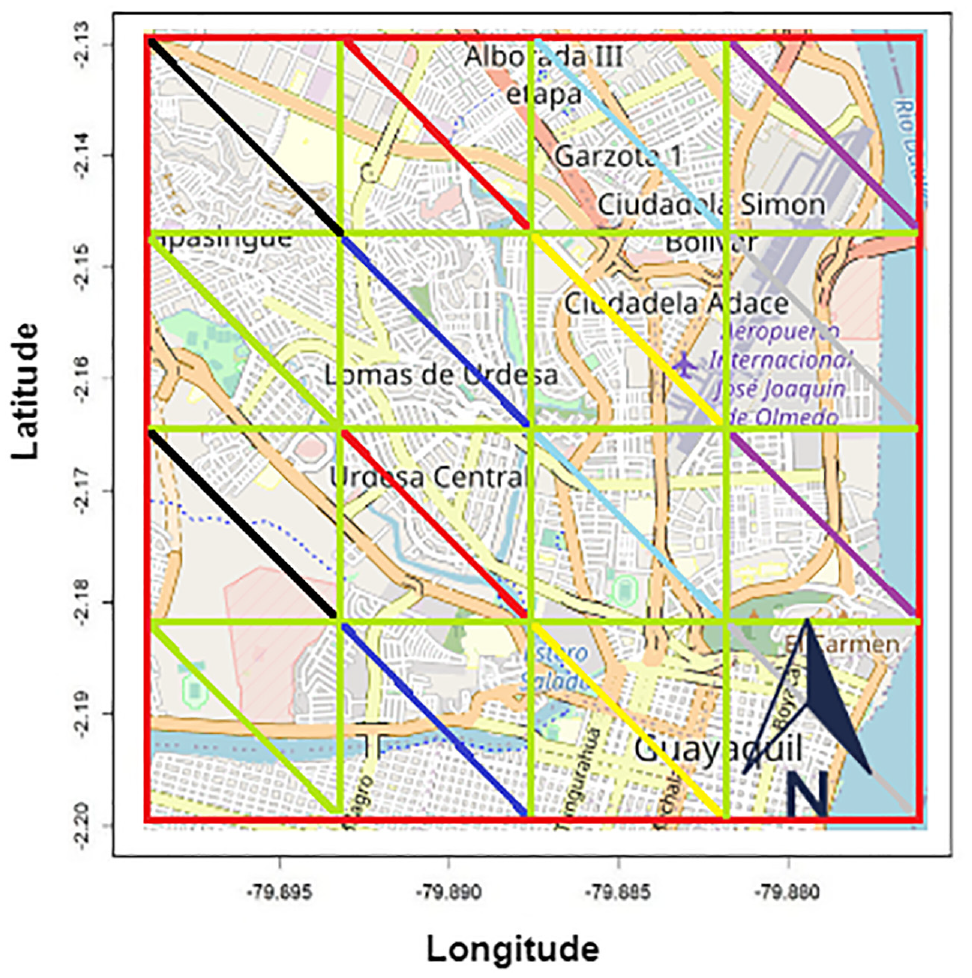
Initial crosslinking and centroid sub-trajectories.

Clustering

The clustering algorithm is an adaptation of the K-means algorithm that operates with sub-trajectories. The new contribution consists of the incorporation of pivots to improve the representation of the centroid in relation to the sub-trajectories of the cluster. Its usefulness is based on the identification of the area in which most sub-trajectories are concentrated within each cell. Although it has a linear plot, its appropriate location within the cell pulls the centroid toward the most representative area.

Following Gao and Leung ( 69 ), in this paper, the Hausdorff distance was used as a similarity measure to assign each sub-trajectory to the closest cluster.

The Hausdorff metric measures the distance between two sub-trajectories of a metric space defined by Rockafellar and Wets ( 70 ). Its use is a result of the need to compare elements made up of several geographical positions.

The process begins with the assignment of each sub-trajectory to the nearest centroid. The initial location of the centroids was indicated immediately after the lattice definition as indicated in the grid setting section. As a result of this assignment process, the first distribution of the sub-trajectories in clusters is formed. From this point on, the sub-trajectories are processed in the context of each cluster. To draw the pivot, it is necessary to identify the area in which most of the sub-trajectories of the cluster are located as well as the main or representative direction of these sub-trajectories.

The plotted area is obtained by arranging the sub-trajectory positions of each group in increasing order in two different lists, one for latitude and one for longitude. The two lists containing all the sub-trajectory positions are divided equally, thus obtaining four lists. The average value of each of these lists is then calculated, generating the following metrics: upper half longitude, lower half longitude, upper half latitude, and lower half latitude.

In the figures, the horizontal axis is associated with longitude, while the vertical axis is associated with latitude.

These values determine four positions: $Pt 1$ (lower half latitude, lower half longitude); $Pt 2$ (upper half latitude, lower half longitude); $Pt 3$ (lower half latitude, upper half longitude); $Pt 4$ (upper half latitude, upper half longitude), as shown in Figure 2.

Figure 2.

Pivot plot area.

In this way, the pivot is plotted in the area where a majority of the sub-trajectories of the cluster are located. The cluster sub-trajectory angles must be averaged to obtain the pivot direction.

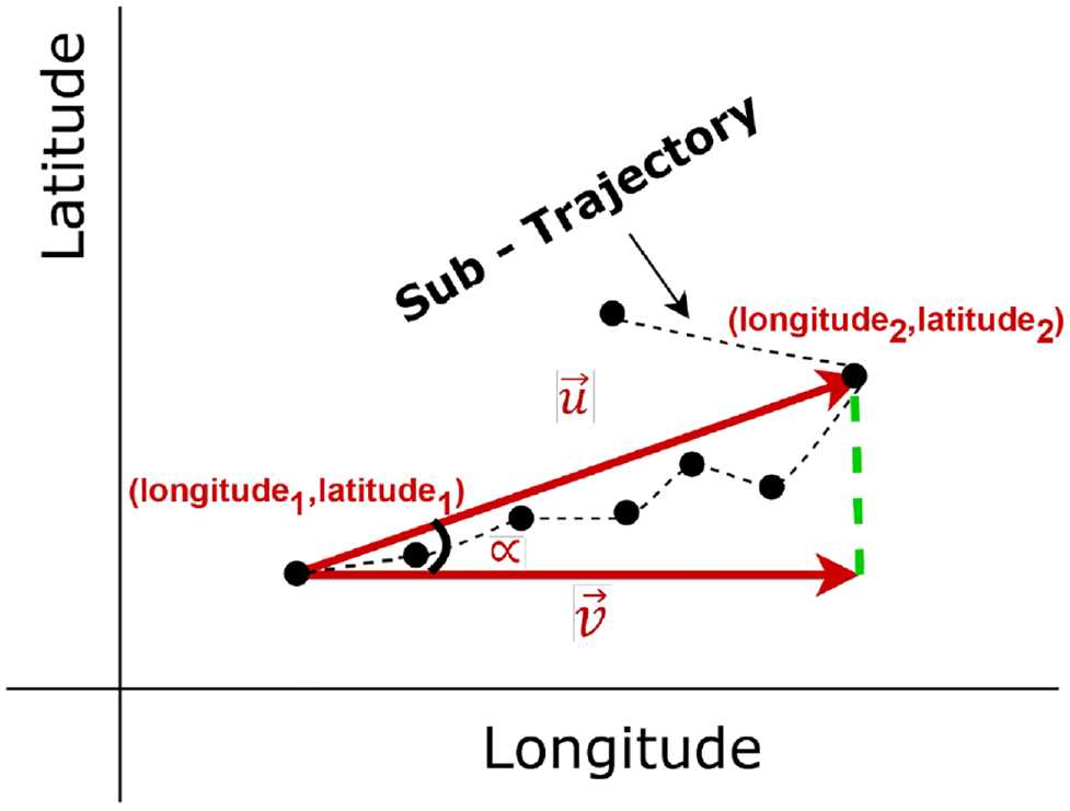
Figure 3 exemplifies the angle $α$ corresponding to a sub-trajectory, with respect to the abscissa axis. Note that, for each sub-trajectory, only their starting position are considered.

Figure 3.

Angle formed by a sub-trajectory with respect to the abscissa axis.

The angle $α$ is computed according to Equation 1, measured in the interval $[- π, π]$

α = \arccos (\frac{\vec{u} \vec{v}}{| \vec{u} | | \vec{v} |})

(1)

Finally, the angles of all sub-trajectories of a cluster are averaged, thus obtaining the angle $φ$ , which defines the direction of the pivot within the plotting area. This angle may be positive or negative, allowing the pivot to be drawn in correspondence with the direction and angle of the sub-trajectories that make up the group.

The pivot trace depends on the sign of the angle. If the mean angle ( $φ$ ) is positive, the mid-position of the lower segment of the constructed area is calculated. On the contrary, if the mean angle ( $φ$ ) is negative, the mid-position of the upper segment is calculated. In each case, starting from that mid-position $(longitud e_{1}, latitud e_{1})$ , the pivot is drawn as illustrated in Figure 4.

Figure 4.

Pivot with: (a) negative; and (b) positive mean angle.

Then, Equation 2 determines the positions of the pivot, where $(longitud e_{1}, latitud e_{1})$ is the previously found mid-position.

latitud e_{1} = \tan φ (longitud e_{1} - longitud e_{2}) + latitud e_{2}

(2)

Each pivot is defined by a given number of positions belonging to the line segment within the previously defined plotting area. This number coincides with the average number of geographic positions that make up the sub-trajectories of the corresponding cluster.

Once the pivot is calculated, it is used as a guide to identify the positions of the sub-trajectories that, when averaged, result in a new centroid position.

Figure 5 shows how the positions are identified following the pivot line. In this figure, $T_{1}$ , $T_{2}$ , and $T_{3}$ represent sub-trajectories, and $P_{1}$ represents the first pivot position to be processed.

Figure 5.

Positions used to determine the centroid.

The process begins with the identification of the position belonging to the closest trajectory ( $T_{1}$ ) to the positions ( $P_{1}$ ) using the Euclidean distance which is also used for data manipulation and trajectory segmentation.

This position is denoted $A_{1}$ in Figure 5. Similarly, positions $B_{1}$ and $C_{1}$ turn out to be the closest to $P_{1}$ for the $T_{2}$ and $T_{3}$ trajectories, respectively. As each of these positions is identified, their latitude and longitude values are stored to calculate their average, once all sub-trajectories in the cluster have been inspected. This average corresponds to the first position of the updated centroid ( $N P_{1}$ ). The remaining positions of the centroid sub-trajectory are calculated in the same way, considering each of the other pivot positions. Therefore, at the end of the centroid update process, the number of positions that make up the centroid matches that of the pivot.

Algorithm 1 summarizes the process described above. The stop or end condition of the algorithm is given by the convergence or stability of the centroids position.

Algorithm 1: Pseudocode of the proposed K-pivot method.
Input: list of sub-trajectories t_List = (t₁, t₂, …, t_n) Output: list of centroids C_List and assignment of each trajectory to CLUSTER_List C_List = (c₁, c₂,…, c_k) ← initial centroids (Figure 1) while stop when the calculated centroid is equal to the current centroid do CLUSTER_List← assign each t_i to the closest centroid using the Hausdorff distance. Calculate the pivots P₁,…, P_k according to centroid updating Subsection // Update each centroid C_i using pivot P_i for i = 1,…, k for each centroid C_i do for each position within pivot P_i do let p_ij be the j–th positions of the pivot P_i for each sub-trajectory of i–th cluster do Find the closest position to p_ij Store latitude and longitude values end for C_ij = Average selected positions end for end for end while

Algorithm 1: Pseudocode of the proposed K-pivot method.

Input: list of sub-trajectories t_List = (t₁, t₂, …, t_n)
Output: list of centroids C_List and assignment of each trajectory to CLUSTER_List
C_List = (c₁, c₂,…, c_k) ← initial centroids (Figure 1)
while stop when the calculated centroid is equal to the current centroid do
CLUSTER_List← assign each t_i to the closest centroid using the Hausdorff distance.
Calculate the pivots P₁,…, P_k according to centroid updating Subsection
// Update each centroid C_i using pivot P_i for i = 1,…, k
for each centroid C_i do
for each position within pivot P_i do
let p_ij be the j–th positions of the pivot P_i
for each sub-trajectory of i–th cluster do
Find the closest position to p_ij
Store latitude and longitude values
end for
C_ij = Average selected positions
end for
end for
end while

Data

The proposed method was implemented in R Language and experiments were carried out on a PC with an Intel core i5-8250 CPU @ 1.60GHz, 8GB RAM, and 64-bit architecture. We ran the experiments on three data sets. The first data set was formed of a series of trajectories recorded by a group of students from the University of Guayaquil using their smartphones. (The Guayaquil dataset is available at https://github.com/gary-reyes-zambrano/Guayaquil-DataSet.git.) The second data set corresponds to a t-drive database and contains information on taxi tours of the city of Beijing (China) and was used by Yuan et al. (71, 72). (The Beijing dataset is available at https://www.microsoft.com/en-us/research/publication/t-drive-trajectory-data-sample/.) The third data set is from “Go! Track” app users in the city of Aracaju (Brazil) and was also used by Zhou et al. ( 73 ) and Tang et al. ( 74 ). (The Aracaju dataset is available at https://archive.ics.uci.edu/ml/machine-learning-databases/00354/.)

Guayaquil Data set

This data set is made up of movement trajectories of university students traveling by public and private means of transport such as taxis, motorcycles, and the metro. It was collected in the city of Guayaquil (Ecuador). It contains positions of approximately 218 users collected in the northern and central Guayaquil cells during October 2017. The positions in this data set were collected by mobile devices with an average time interval between two consecutive positions of 5 s. This data set was pre-processed to extract records from October 28 from 16:30 to 18:30 as during this period, there was the highest concentration of positions in the data set. After filtering, we obtained 30,557 records, representing 206 trajectories. The file format in the repository has the following fields: id trajectory, latitude, longitude, and time stamp (unix time). Figure 6 shows a representation of the data set on the map of the city of Guayaquil.

Figure 6.

Geographic representation of the data set from Guayaquil.

Beijing Data Set

This data set consists of taxi tours in the city of Beijing (China). The data set comes from the t-drive project and contains the positions of 10,357 taxis collected in Beijing during February 2008. The positions in this data set were collected by taxi GPS devices with an average time interval between two consecutive positions of 177 s. This data set was pre-processed to extract the records from February 02 from 13:30 to 15:00 to focus the experiment within a certain time frame. After this filtering process, 62,138 records were obtained, representing 630 trajectories. The file formats in the repository are as follows: trajectory id, date-time, longitude, and latitude. A representation of the Beijing city map is shown in Figure 7.

Figure 7.

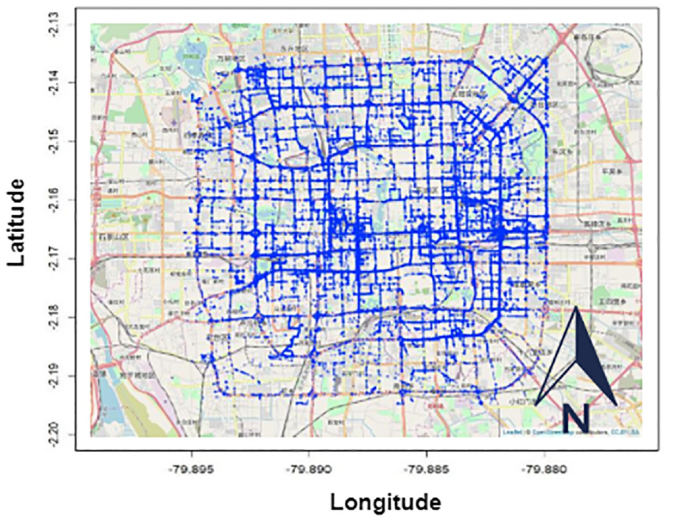
Geographic representation of the data set from Beijing.

Aracaju Data Set

The third data set consists of car and bus user routes recorded through the “Go! Track” app in the city of Aracaju (Brazil). The data set includes trajectories collected in Aracaju from September 13, 2014 to January 19, 2016. The positions in this data set were collected with high time variability between two consecutive positions. This data set was pre-processed to extract the records from September 13, 2014, 07:24:32 to July 23, 2015, 09:27:51. After filtering, 14,096 records were obtained representing 137 trajectories. The format of the files in the repository are as follows: id, latitude, longitude, and track_id, time. A representation of the data set on the city map of Aracaju is shown in Figure 8.

Figure 8.

Geographic representation of the data set from Aracaju.

Obtained Results

The central contribution of the K-pivot clustering technique proposed in this paper lies precisely in the use of a pivot. Its performance was compared with two existing solutions in the literature: the clustering of trajectories using the K-means method adapted for trajectories (in this work is called K-centroids) and a density-based clustering using the Tra-DBScan method.

During the iterative update process of the K-centroid algorithm, each sub-trajectory is directly compared with the previous centroid and then recalculated. As for Tra-DBScan, it uses the concept of neighborhood to define whether a sub-trajectory should be incorporated into an existing cluster or not; it also requires a minimum number of sub-trajectories for a cluster to be formed.

On the number of cells that make up the lattice, as previously mentioned, its value depends on the precision with which the analysis of the trajectories is to be carried out. The fewer cells used, the larger the coverage area of each cell and the less accurate the information or description of the centroids. In this paper, several experiments were performed with sizes ranging from $2 \times 2$ to $16 \times 16$ . In each case, to select the cell size, the performance of the algorithm was analyzed along with a silhouette index value for the quality of the obtained clusters. The results obtained with a lattice of $4 \times 4$ were satisfactory so it was decided to use this value. If a higher level of detail is required, the number of lattice cells should be increased. Thus, this lattice generates 16 evenly distributed cells.

Table 2 shows the results obtained after the execution of the proposed K-pivot method with the three sets of positions data (Beijing, Guayaquil, and Aracaju). The 16 groups formed by the method are shown together with the percentage of sub-trajectories assigned to each group.

Table 2.

Percentage of Sub-Trajectories Assigned to Each Given Group

Groups	Beijing (%)	Guayaquil (%)	Aracaju (%)
1	5.91	0.93	3.23
2	5.72	2.14	9.26
3	3.94	4.77	5.61
4	5.88	2.05	3.30
5	7.49	1.66	9.61
6	5.68	16.50	15.52
7	6.21	4.64	3.25
8	5.00	3.79	9.31
9	11.82	2.48	2.93
10	9.62	3.92	7.65
11	3.57	14.19	0.02
12	5.42	7.16	1.69
13	8.19	6.11	5.44
14	6.91	7.52	10.58
15	4.63	6.43	2.96
16	4.00	15.72	9.61

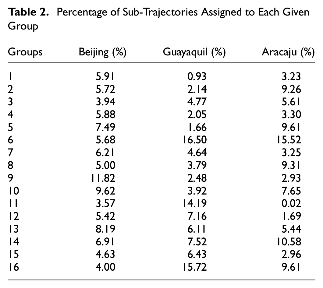
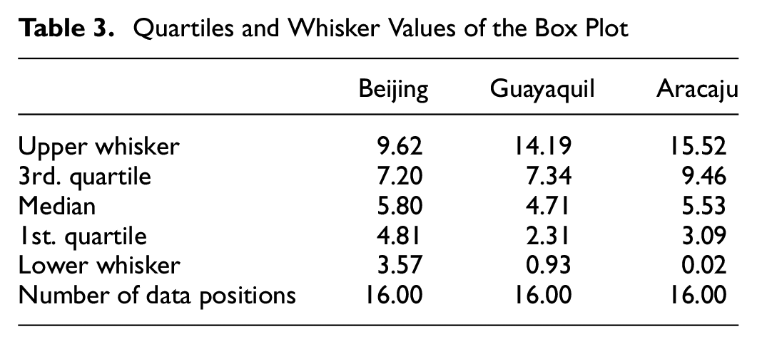
The box plot displayed in Figure 9, constructed from the percentages in Table 2, shows that the proposed method adequately distributes the sub-trajectories among all the clusters. It is observed that although groups of different sizes are generated, only one in the case of the Beijing base and two in the case of the Guayaquil base, are much larger than the rest. This is because of the use of the initial lattice where a pivot was located in each square, which allowed a uniform inspection of the entire area of interest.Table 3 shows the quartiles and whisker values of the box plot.

Table 3.

Quartiles and Whisker Values of the Box Plot

	Beijing	Guayaquil	Aracaju
Upper whisker	9.62	14.19	15.52
3rd. quartile	7.20	7.34	9.46
Median	5.80	4.71	5.53
1st. quartile	4.81	2.31	3.09
Lower whisker	3.57	0.93	0.02
Number of data positions	16.00	16.00	16.00

Figure 9.

Boxplot of the percentages of the sub-trajectories.

Figure 10 shows the clusters obtained by each of the data sets (Guayaquil, Aracaju, and Beijing respectively) with the proposed K-pivot method.

Figure 10.

Clusters determined with the proposed K-pivot method.

Validation

The Silhouette index ( 75 ), considering the Hausdorff distance to compare two sub-trajectories, is used to validate the clustering results. Equation 3 indicates how to calculate the Silhouette index for the $i$ -th sub-trajectory:

s (i) = \frac{b (i) - a (i)}{max {a (i), b (i)}}

(3)

where $a (i)$ is the average distance from the $i -$ th sub-trajectory to all other sub-trajectories in the same cluster, and $b (i)$ is the average distance from the $i -$ th sub-trajectory to all other sub-trajectories belonging to the closest group. Then, $s (i)$ is the Silhouette index of the $i -$ th sub-trajectory. This index ranges from $- 1$ to $+ 1$ , with the cluster with the highest value being the best. The average of the silhouette indices of all sub-trajectories is then calculated to obtain the corresponding cluster index.

Table 4 summarizes the values of the average silhouette indexes for each cluster for the proposed and the benchmark methods. As can be seen, the silhouette indices of the proposed K-pivot method are slightly higher than the obtained K-centroid and Tra-DBScan methods.

Table 4.

Average Silhouette Index for Each Method

	Beijing	Guayaquil	Aracaju
Number of sub-trajectories (segmented)	19,245	9,530	4,026
Silhouette (K-pivot)	0.3455	0.4647	0.4946
Silhouette (K-centroid)	0.3392	0.4549	0.4820
Silhouette (Tra-DBScan)	0.1604	0.3248	0.4491

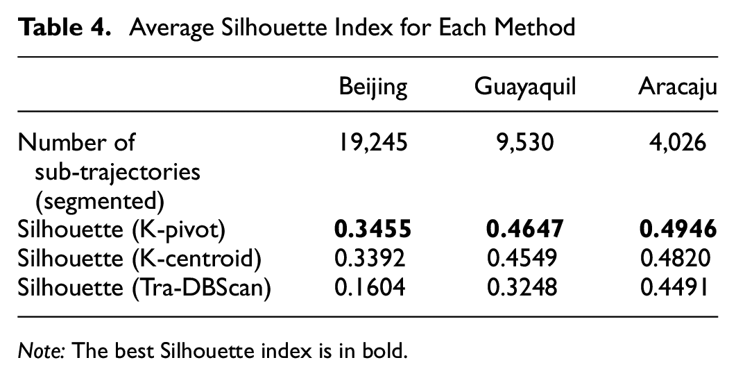
Note: The best Silhouette index is in bold.

Given that the silhouette indices obtained by the K-pivot and K-centroid methods do not show significant differences, it was also proposed to analyze, for both methods, the interquartile ranges of the silhouette indices of the sub-trajectories that make up each group once the process was completed.

It is important to note that both methods start with the same lattice. It is also noteworthy that, if the lattice cells were numbered from 1 to 16, a direct correspondence would be observed between the centroids of both methods. That is, for example, the first centroid of the cluster generated by K-pivot would correspond to sub-trajectories of the first cell of the map as well as the first centroid of the cluster generated with K-centroid. This was verified for all cells. On this basis, it was possible to directly compare the silhouette indices of the $i -$ th cluster using the K-pivot method with the $i -$ th cluster using the K-centroid method.

Then, the pairwise clusters are compared: the $i -$ th cluster generated by K-pivot and the $i -$ th cluster generated by K-centroid. A ranking is considered to be better if the Silhouette indices of the sub-trajectories composing a cluster result in a smaller interquartile range and higher values for both the first and third quartiles. This criterion indicates that 50% of the sub-trajectories of the cluster considered to be “better” have lower dispersion and a higher silhouette index value. Consequently, they could be considered to be of better clustering quality.

Table 5 shows the results obtained by applying the K-pivot and K-centroid methods to the Beijing data. It can be seen that 64.97% of the groups generated with the proposed method, K-pivot, comply with the characteristics mentioned for the interquartile range and the quartiles that limit the box of the corresponding diagram. On the other hand, the K-centroid method does the same for the remaining 35.03% of the groups. This shows that the proposed method generates groups with lower dispersion and greater separation between clusters.

Table 5.

Interquartile Range of the First and Third Quartiles of Silhouette

	Beijing (%)	Guayaquil (%)	Aracaju (%)
K-pivot	64.97	60.92	52.91
K-centroid	35.03	39.08	47.09

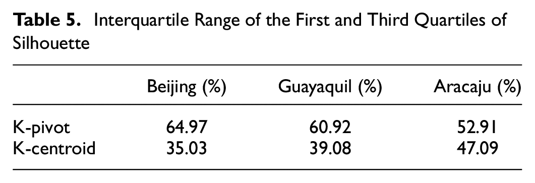
Based on the results reported in Table 4 and the comparison observed in Table 5, we thus find that the incorporation of the pivot improves the quality of the clustering.

Conclusions

The key contribution of the K-pivot clustering technique proposed in the present paper lies precisely in the use of a pivot as a guide for the recalculation of each centroid.

To plot the pivot, the area of highest sub-trajectory concentration of the cluster is taken into account together with the corresponding average direction. The proposed method uses the segmentation strategy defined by Reyes-Zambrano et al. ( 44 ) which allows shorter sub-trajectories with minor direction changes to be used. To establish the position of the initial centroids, a regular lattice was used to ensure its uniform distribution in the area under study.

The proposed method was compared with a variant of the K-means algorithm adapted for the treatment of sub-trajectories called K-centroid, as well as with the Tra-DBScan method. The clusters obtained with the proposed K-pivot method were distributed over the area under study. The quality of the clustering results of the sub-trajectories obtained by the K-pivot method using the silhouette index was satisfactory. Furthermore, the comparison with the Tra-DBScan method reveals the influence of the lattice on the results. The clusters obtained with the proposed K-pivot algorithm are uniformly distributed in the area under study, while those generated by Tra-DBScan are concentrated in specific positions. The quality of the clustering results for the sub-trajectories obtained by means of the silhouette index were satisfactory. In fact, the introduction of the pivot improves the quality of the clustering. In this way, it will be possible to characterize the different sectors of the map that the trajectories cover, identifying possible levels of congestion.

The proposed method can identify a conglomerated trajectory that can be indicative of traffic congestion, even detecting the vehicular flow levels in avenues or main roads, in peak hours mainly, or any other situation such as an accident or any traffic stoppage. The method gives the direction of the traffic and this information is important for decision making and can focus the resulting cluster in an specific area in a road map.

In the future, it is proposed to make adaptations in the way the pivot orientation is defined. This will include other sub-trajectory characteristics that may influence both its direction and angle. It is also intended to evaluate the results of clustering using dynamic clustering algorithms in which it is not necessary to define initial centroids for the identification of patterns.

Footnotes

Author Contributions

The authors confirm contribution to the paper as follows: study conception and design: Gary Reyes, Laura Lanzarini, Waldo Hasperué; data collection: Gary Reyes; analysis and interpretation of results: Gary Reyes, Laura Lanzarini, Waldo Hasperué, Aurelio F. Bariviera; draft manuscript preparation: Gary Reyes, Laura Lanzarini, Waldo Hasperué, Aurelio F. Bariviera. All authors reviewed the results and approved the final version of the manuscript.

Declaration of Conflicting Interests

The author(s) declared no potential conflicts of interest with respect to the research, authorship, and/or publication of this article.

Funding

The author(s) received no financial support for the research, authorship, and/or publication of this article.

ORCID iDs

Waldo Hasperué

Aurelio F. Bariviera

Data Accessibility Statement

Guayaquil data set is available at https://github.com/gary-reyes-zambrano/Guayaquil-Dataset.git. Beijing data set is available at >https://www.microsoft.com/en-us/research/publication/t-drive-trajectory-data-sample/. Aracaju data set is available at

References

Kang

J. H.

Welbourne

Stewart

Borriello

Extracting Places from Traces of Locations. Proc., 2nd ACM International Workshop on Wireless Mobile Applications and Services on WLAN Hotspots. WMASH ‘04, Association for Computing Machinery, New York, NY, 2004, pp. 110–118.

Zheng

Xie

Chen

Liu

W.-Y.

Mining User Similarity Based on Location History. Proc., 16th ACM SIGSPATIAL International Conference on Advances in Geographic Information Systems. GIS ‘08, Association for Computing Machinery, New York, NY, 2008, pp. 1–10.

Varghese

B. M.

Unnikrishnan

Poulose

J. K.

Spatial clustering algorithms – An overview. Asian Journal of Computer Science and Information Technology, Vol. 3, No. 1, 2013, pp. 1–8.

James

R. M.

Hammit

B. E.

Identifying Contributory Factors to Heterogeneity in Driving Behavior: Clustering and Classification Approach. Transportation Research Record: Journal of the Transportation Research Board, 2019. 2673: 343–353.

Mazimpaka

J. D.

Timpf

Trajectory Data Mining: A Review of Methods and Applications. Journal of Spatial Information Science, Vol. 13, No. 13, 2016, pp. 61–99. https://doi.org/10.5311/JOSIS.2016.13.263.

Markovi

Sekuła

Laan

Z. V.

Andrienko

Applications of Trajectory Data from the Perspective of a Road Transportation Agency : Literature Review and Maryland Case Study. IEEE Transactions on Intelligent Transportation Systems, Vol. 20, No. 5, 2019, pp. 1858–1869.

Tang

Zhu

Huang

Peng

Z.-r.

Wang

Identification and Interpretation of Spatial – Temporal Mismatch Between Taxi Demand and Supply Using Global Positioning System Data. Journal of Intelligent Transportation Systems, 2018, pp. 403–415. https://doi.org/10.1080/15472450.2018.1518137.

Yuan

Zhu

Yang

Xie

Behavioral Responses to Pre-Planned Road Capacity Reduction Based on Smartphone GPS Trajectory Data : A Functional Data Analysis Approach. Journal of Intelligent Transportation Systems, 2018, pp. 1–11. https://doi.org/10.1080/15472450.2018.1488133.

Bathaee

Mohseni

Park

Porter

J. D.

Kim

D. S.

Bathaee

Mohseni

Park

Porter

J. D.

David

A Cluster Analysis Approach for Differentiating Transportation Modes Using Bluetooth Sensor Data. Journal of Intelligent Transportation Systems, Vol. 22, No. 4, 2018, pp. 353–364. https://doi.org/10.1080/15472450.2018.1457444.

10.

Bartin

Ozbay

Iyigun

Clustering-Based Methodology for Determining Optimal Roadway Configuration of Detectors for Travel Time Estimation. Transportation Research Record: Journal of the Transportation Research Board, 2007. 2000: 98–105.

11.

Hans

Chiabaut

Leclercq

Clustering Approach for Assessing the Travel Time Variability of Arterials. Transportation Research Record: Journal of the Transportation Research Board, 2014. 2422: 42–49.

12.

Filipovska

Mahmassani

H. S.

Mittal

Estimation of Path Travel Time Distributions in Stochastic Time-Varying Networks with Correlations. Transportation Research Record: Journal of the Transportation Research Board, 2021. 036119812110184.

13.

Zhang

Han

L. D.

Kim

Dijkstra’s-DBSCAN: Fast, Accurate, and Routable Density Based Clustering of Traffic Incidents on Large Road Network. Transportation Research Record: Journal of the Transportation Research Board, 2018. 2672: 265–273.

14.

Pascale

Mavroeidis

Lam

H. T.

Spatiotemporal Clustering of Urban Networks: Real Case Scenario in London. Transportation Research Record: Journal of the Transportation Research Board, 2015. 2491: 81–89.

15.

Lloyd

Least squares quantization in PCM. IEEE Transactions on Information Theory, Vol. 28, No. 2, 1982, pp. 129–137.

16.

Hartigan

J. A.

Wong

M. A.

Algorithm AS 136: A K-Means Clustering Algorithm. Journal of the Royal Statistical Society. Series C (Applied Statistics), Vol. 28, No. 1, 1979, pp. 100–108.

17.

Wang

Song

Pan

Using Taxi GPS Trajectory Data to Optimize the Spatial Layout of Urban Taxi Stands. Transportation Research Record: Journal of the Transportation Research Board, 2021. 2675: 301–312.

18.

Madhulatha

T. S.

An Overview on Clustering Methods. IOSR Journal of Engineering, Vol. 2, No. 4, 2012, pp. 719–725.

19.

Jain

A. K.

Data Clustering: 50 Years Beyond K-means. Pattern Recognition Letters, Vol. 31, No. 8, 2010, pp. 651–666. https://doi.org/10.1016/j.patrec.2009.09.011.

20.

Tork

H. F.

Spatio-Temporal Clustering Methods Classification. Proc., 7th Doctoral Symposium in Informatics Engineering ( Oliveira

David

Sousa

A. A.

, eds), FEUP Edições, 2012, pp. 199–209. https://doi.org/10.13140/RG.2.1.3812.7204.

21.

Han

Kamber

Tung

A. K. H.

Spatial Clustering Methods in Data Mining: A Survey. In Geographic Data Mining and Knowledge Discovery, Research Monographs in GIS ( Miller

H. J.

Han

, eds), Taylor and Francis, 2001, pp. 188–217. http://www-faculty.cs.uiuc.edu/hanj/pdf/gkdbk01.pdf.

22.

Lee

J.-G.

Han

Incremental Clustering for Trajectories. Proc., DASFAA’10: 15th International Conference on Database Systems for Advanced Applications, Tsukuba, Japan, 2010, pp. 32–46.

23.

Aggarwal

C. C.

P. S.

Han

Wang

- A Framework for Clustering Evolving Data Streams. In Proceedings 2003 VLDB Conference ( Freytag

J.-C.

Lockemann

Abiteboul

Carey

Selinger

Heuer

, eds), Morgan Kaufmann, San Francisco, 2003, pp. 81–92.

24.

Oliveira

L. K.

Barraza

B. V. B.

C. A. I.

An Overview of Problems and Solutions for Urban Freight Transport in Brazilian Cities. Sustainability, Vol. 10, No. 1233, 2018, pp. 1–14. https://doi.org/10.3390/su10041233.

25.

Erman

Arlitt

Mahanti

Methodologies

I. C.

Recognition

Traffic Classification Using Clustering Algorithms. In MineNet ‘06: Proceedings of the 2006 SIGCOMM Workshop on Mining Network Data, Pisa, Italy, 2006, pp. 281–286.

26.

Wang

Qin

Chen

Zhao

Detecting Anomalous Trajectories and Behavior Patterns Using Hierarchical Clustering from Taxi GPS Data. International Journal of Geo-Information, Vol. 7, No. 25. https://doi.org/10.3390/ijgi7010025.

27.

Zheng

. Trajectory Data Mining : An Overview. ACM Trans. On Intelligent Systems and Technology, Vol. 6, No. 3, pp. 1–41. https://doi.org/10.1145/2743025.

28.

Gaffney

Smyth

Trajectory Clustering With Mixtures of Regression Models. Proc., 5th ACM SIGKDD International Conference on Knowledge Discovery and Data Mining - KDD ‘99. ACM Press, 1999, pp. 63–72.

29.

Zhou

Miao

Zhang

Gong

A Trajectory Regression Clustering Technique Combining a Novel Fuzzy C-Means Clustering Algorithm With the Least Squares Method. ISPRS International Journal of Geo-Information, Vol. 7, No. 5, p. 164. https://doi.org/10.3390/ijgi7050164.

30.

Nanni

. Clustering Methods for Spatio-Temporal Data. PhD thesis. Department Computer Science, University Pisa, 2002.

31.

Ester

Kriegel

H.-P.

Sander

A Density-Based Algorithm for Discovering Clusters in Large Spatial Databases with Noise. In Proceedings of the Second International Conference on Knowledge Discovery and Data Mining ( Evangelos Simoudis

U. M. F.

Han

, eds), KDD’96, AAAI Press, 1996, pp. 226–231.

32.

Choong

M. Y.

Chin

R. K. Y.

Yeo

K. B.

Teo

K. T. K.

Trajectory Pattern Mining Via Clustering Based on Similarity Function for Transportation Surveillance. International Journal of Simulation-Systems, Science & Technology, Vol. 17, No. 34, 2016, pp. 19.1–19.7.

33.

Kim

Mahmassani

H. S.

Spatial and Temporal Characterization of Travel Patterns in a Traffic Network Using Vehicle Trajectories. Transportation Research Procedia, Vol. 9, 2015, pp. 164–184.

34.

Yuan

Raubal

Measuring Similarity of Mobile Phone User Trajectories–A Spatio-Temporal Edit Distance Method. International Journal of Geographical Information Science, Vol. 28, No. 3, 2014, pp. 496–520.

35.

Luo

Zheng

Ren

An Improved DBSCAN Algorithm to Detect Stops in Individual Trajectories. ISPRS International Journal of Geo-Information, Vol. 6, No. 3, 2017, p. 63. https://doi.org/10.3390/ijgi6030063.

36.

Liu

Yan

Research on Evaluation Function of Clustering Algorithm Based on Duty Cycle. In Proceedings - International Computer Software and Applications Conference ( Getov

Gaudiot

J.-L.

Yamai

Cimato

Chang

Teranishi

Yang

J.-J.

Leong

Shahriar

Takemoto

Towey

Takakura

Elci

Takeuchi

Puri

, eds), IEEE Computer Society, 2019, Vol. 2, pp. 48–54.

37.

Zheng

Xia

Zhao

Tan

Chen

Liu

Spatial–Temporal Travel Pattern Mining Using Massive Taxi Trajectory Data. Physica A: Statistical Mechanics and its Applications, Vol. 501, 2018, pp. 24–41. https://doi.org/10.1016/j.physa.2018.02.064.

38.

Liu

L. X.

Song

J. T.

Guan

Z. X.

K. J.

Tra-DBScan: A Algorithm of Clustering Trajectories. Applied Mechanics and Materials, Vol. 121–126, 2011, pp. 4875–4879. https://doi.org/10.4028/www.scientific.net/AMM.121-126.4875.

39.

Ferreira

Klosowski

J. T.

Scheidegger

C. E.

Silva

C. T.

Vector Field k-Means: Clustering Trajectories by Fitting Multiple Vector Fields. Computer Graphics Forum, Vol. 32, No. 3pt2, 2013, pp. 201–210. https://doi.org/10.1111/cgf.12107.

40.

Buchin

Driemel

Van De L’Isle

Nusser

Klcluster: Center-Based Clustering of Trajectories. In GIS: Proceedings of the ACM International Symposium on Advances in Geographic Information Systems ( Banaei-Kashani

Trajcevski

Guting

Kulik

Newsam

, eds), Association for Computing Machinery, 2019, pp. 496–499. https://doi.org/10.1145/3347146.3359111.

41.

Choong

Angeline

Chin

Yeo

Teo

Modeling of Vehicle Trajectory Using K-Means And Fuzzy C-means Clustering. Proc., 2018 IEEE International Conference on Artificial Intelligence in Engineering and Technology, Institute of Electrical and Electronics Engineers Inc., 2019, pp. 1–6.

42.

Luo

Chen

Trajectory Similarity Clustering Based on Multi-Feature Distance Measurement. Applied Intelligence, Vol. 49, No. 6, 2019, p. 2315–2338. https://doi.org/10.1007/s10489-018-1385-x.

43.

Yang

Cai

Yang

Zhang

Zhao

TAD: A Trajectory Clustering Algorithm Based on Spatial-Temporal Density Analysis. Expert Systems with Applications, Vol. 139, 2020, p. 112846. https://doi.org/10.1016/j.eswa.2019.112846.

44.

Reyes-Zambrano

Lanzarini

Hasperué

Bariviera

A. F.

GPS Trajectory Clustering Method for Decision Making on Intelligent Transportation Systems. Journal of Intelligent & Fuzzy Systems, Vol. 38, No. 5, 2020, pp. 5529–5535. https://doi.org/10.3233/JIFS-179644.

45.

Lee

J.-G.

Han

Whang

K.-Y.

Trajectory Clustering: A Partition-and-Group Framework. Proc., 2007 ACM SIGMOD International Conference on Management of Data. SIGMOD ‘07, Association for Computing Machinery, 2007, pp. 593–604. https://doi.org/10.1145/1247480.1247546.

46.

Ailin

Zhong

Dechao

Movement Pattern Extraction Based on a Non-parameter Sub-trajectory Clustering Algorithm. Proc., IEEE 4th International Conference on Big Data Analytics (ICBDA). Suzhou, China, IEEE, 2019, pp. 5–9.

47.

Mao

Zhong

Ping

An Adaptive Trajectory Clustering Method Based on Grid and Density in Mobile Pattern Analysis. Sensors, Vol. 17, No. 9, 2017, p. 2013. https://doi.org/10.3390/s17092013.

48.

Wang

Xiao

Segmented Trajectory Clustering-Based Destination Prediction in IoVs. IEEE Access, Vol. 8, 2020, pp. 98999–99009. https://doi.org/10.1109/ACCESS.2020.2998063.

49.

Shukla

Tripathi

A Multi-Tier Based Clustering Framework for Scalable and Energy Efficient WSN-Assisted IoT Network. Wireless Networks, Vol. 26, No. 5, 2020, pp. 3471–3493. https://doi.org/10.1007/s11276-020-02277-4.

50.

Hong

Chen

Mahmassani

H. S.

Recognizing Network Trip Patterns Using a Spatio-Temporal Vehicle Trajectory Clustering Algorithm. IEEE Transactions on Intelligent Transportation Systems, Vol. 19, No. 8, 2018, p. 2548–2557. https://doi.org/10.1109/TITS.2017.2754401.

51.

Discovering Frequent Movement Paths From Taxi Trajectory Data Using Spatially Embedded Networks and Association Rules. IEEE Transactions on Intelligent Transportation Systems, Vol. 20, No. 3, 2019, p. 855–866. https://doi.org/10.1109/TITS.2018.2834573.

52.

Feng

Bai

Identification of Critical Roads in Urban Transportation Network Based on GPS Trajectory Data. Physica A: Statistical Mechanics and its Applications, Vol. 535, 2019, p. 122337. https://doi.org/10.1016/j.physa.2019.122337.

53.

Niu

Chen

C. Q.

Niu

Label-Based Trajectory Clustering in Complex Road Networks. IEEE Transactions on Intelligent Transportation Systems, Vol. 21, No. 10, 2020, p. 4098–4110. https://doi.org/10.1109/TITS.2019.2937882.

54.

Xiong

Shang

Bian

Detecting Intrinsic Dynamics of Traffic Flow With Recurrence Analysis and Empirical Mode Decomposition. Physica A: Statistical Mechanics and its Applications, Vol. 474, 2017, pp. 70–84. https://doi.org/10.1016/j.physa.2017.01.060.

55.

Wang

Chow

C.-Y.

Lyu

Lee

V. C. S.

Kwong

Zeng

TaxiRec: Recommending Road Clusters to Taxi Drivers Using Ranking-Based Extreme Learning Machines. Proc., 23rd SIGSPATIAL International Conference on Advances in Geographic Information Systems, Beijing, China, ACM, 2015, pp. 1–4.

56.

Tallapragada

Cortes

Hierarchical-Distributed Optimized Coordination of Intersection Traffic. IEEE Transactions on Intelligent Transportation Systems, Vol. 21, No. 5, 2020, pp. 2100–2113. https://doi.org/10.1109/TITS.2019.2912881.

57.

Huang

Xiao

Wang

Jiang

Exploring Individual Travel Patterns Across Private Car Trajectory Data. IEEE Transactions on Intelligent Transportation Systems, Vol. 21, No. 12, 2020, pp. 5036–5050. https://doi.org/10.1109/TITS.2019.2948188.

58.

Tang

Liu

Zhang

Exploring Urban Travel Patterns Using Density-Based Clustering With Multi-Attributes from Large-Scaled Vehicle Trajectories. Physica A: Statistical Mechanics and its Applications, Vol. 561, 2021, P. 125301. https://doi.org/10.1016/j.physa.2020.125301.

59.

Kumar

Rajasegarar

Leckie

Krishnaswamy

Palaniswami

Fast and Scalable Big Data Trajectory Clustering for Understanding Urban Mobility. IEEE Transactions on Intelligent Transportation Systems, Vol. 19, No. 11, 2018, pp. 3709–3722. https://doi.org/10.1109/TITS.2018.2854775.

60.

Rathore

Kumar

Rajasegarar

Palaniswami

Bezdek

J. C.

A Scalable Framework for Trajectory Prediction. IEEE Transactions on Intelligent Transportation Systems, Vol. 20, No. 10, 2019, pp. 3860–3874. https://doi.org/10.1109/TITS.2019.2899179.

61.

Qiao

Han

Zhu

Gutierrez

L. A.

TraPlan: An Effective Three-in-One Trajectory-Prediction Model in Transportation Networks. IEEE Transactions on Intelligent Transportation Systems, Vol. 16, No. 3, 2015, pp. 1188–1198. https://doi.org/10.1109/TITS.2014.2353302.

62.

Liu

Zhang

Adaptive Density Trajectory Cluster Based on Time and Space Distance. Physica A: Statistical Mechanics and its Applications, Vol. 484, 2017, pp. 41–56. https://doi.org/10.1016/j.physa.2017.04.119.

63.

Yuan

Sun

Zhao

Wang

A Review of Moving Object Trajectory Clustering Algorithms. Artificial Intelligence Review, Vol. 47, No. 1, 2017, pp. 123–144. https://doi.org/10.1007/s10462-016-9477-7.

64.

Xing

E. P.

A. Y.

Jordan

M. I.

Russell

Distance Metric Learning, With Application to Clustering With Side-Information. Proc., 15th International Conference on Neural Information Processing Systems, NIPS’02, MIT Press, Cambridge, MA, 2002, pp. 521–528.

65.

Thakare

Bagal

Performance Evaluation of K-means Clustering Algorithm With Various Distance Metrics. International Journal of Computer Applications, Vol. 110, No. 11, 2015, pp. 12–16.

66.

Besse

P. C.

Guillouet

Loubes

J.-M.

Royer

Review and Perspective for Distance-Based Clustering of Vehicle Trajectories. IEEE Transactions on Intelligent Transportation Systems, Vol. 17, No. 11, 2016, pp. 3306–3317. https://doi.org/10.1109/TITS.2016.2547641.

67.

Magdy

Sakr

M. A.

Mostafa

El-Bahnasy

Review on Trajectory Similarity Measures. Proc., 2015 IEEE 7th International Conference on Intelligent Computing and Information Systems (ICICIS), Cairo, Egypt, 2015, pp. 613–619.

68.

Zhang

Guo

Pei

Deep Trajectory Similarity Model: A Fast Method for Trajectory Similarity Computation. Proc., International Conference on Transportation and Development 2019, American Society of Civil Engineers, Reston, VA, 2019, pp. 13–23.

69.

Gao

Leung

M. K. H.

Line Segment Hausdorff Distance on Face Matching. Pattern Recognition, Vol. 35, No. 2, 2002, pp. 361–371. https://doi.org/10.1016/S0031-3203(01)00049-8.

70.

Rockafellar

R. T.

Wets

R. J.-B.

Variational Analysis. Vol. 317, Springer-Verlag, 2009.

71.

Yuan

Zheng

Zhang

Xie

Sun

Huang

T-Drive: Driving Directions Based on Taxi Trajectories. Proc., 18th SIGSPATIAL International Conference on Advances in Geographic Information Systems, San Jose, CA, 2010, pp. 99–108.

72.

Yuan

Zheng

Xie

Sun

Driving With Knowledge from the Physical World. Proc., 17th ACM SIGKDD International Conference on Knowledge Discovery and Data Mining, San Diego, CA, 2011, pp. 316–324.

73.

Zhou

Shen

Miao

Zhang

Gong

An Automatic K-means Clustering Algorithm of GPS Data Combining a Novel Niche Genetic Algorithm With Noise and Density. ISPRS International Journal of Geo-Information, Vol. 6, No. 12, 2017, p. 392.

74.

Tang

Liu

Wang

Uncovering Urban Human Mobility from Large Scale Taxi GPS Data. Physica A: Statistical Mechanics and its Applications, Vol. 438, 2015, pp. 140–153.

75.

Rousseeuw

P. J.

Silhouettes: A Graphical Aid to the Interpretation and Validation of Cluster Analysis. Journal of Computational and Applied Mathematics, Vol. 20, 1987, pp. 53–65. https://doi.org/10.1016/0377-0427(87)90125-7.