Deep-Learning Spatiotemporal Prediction Framework for Particulate Matter under Dynamic Monitoring

Data and Methods

For the modeling based on historical data, secondary data in the form of pollutant concentrations and meteorological parameters is collected from the Central Pollution Control Board (CPCB) ( 29 ). Hourly data from multiple air pollution monitoring stations is collected for January 2019 to April 2021. There were no monitors in South Delhi before the year 2019, and therefore, historical data for 2019 to 2021 is considered in the present study ( 29 ). Meteorological parameters are included in prediction models as these parameters are likely to influence the pollutant concentrations significantly ( 30 ). Particulate matter, PM2.5 and PM10 (in μg/m³), and meteorological parameters, such as temperature (in °C), barometric pressure (in mm Hg), humidity (in %), wind speed (m/s), and wind direction are used in this study. The clockwise angle from the north defines the wind direction.

The hourly variations of PM2.5 and PM10 concentrations of the four static monitors on two different days in different seasons are shown in Figure 1. It can be observed that PM2.5 and PM10 concentrations are high in November (winter season) compared with June (summer season), for various reasons. At the same time, the value varies significantly with the time of the day. Increased local emissions from crop and biomass waste burning, winter inversion (low wind speed with dip in temperature leading to accumulated pollutants at lower height), and absence of photochemical reactions in winter assists in increased concentrations in the winter season compared with summer ( 31 ).

OPEN IN VIEWER

Figure 1.

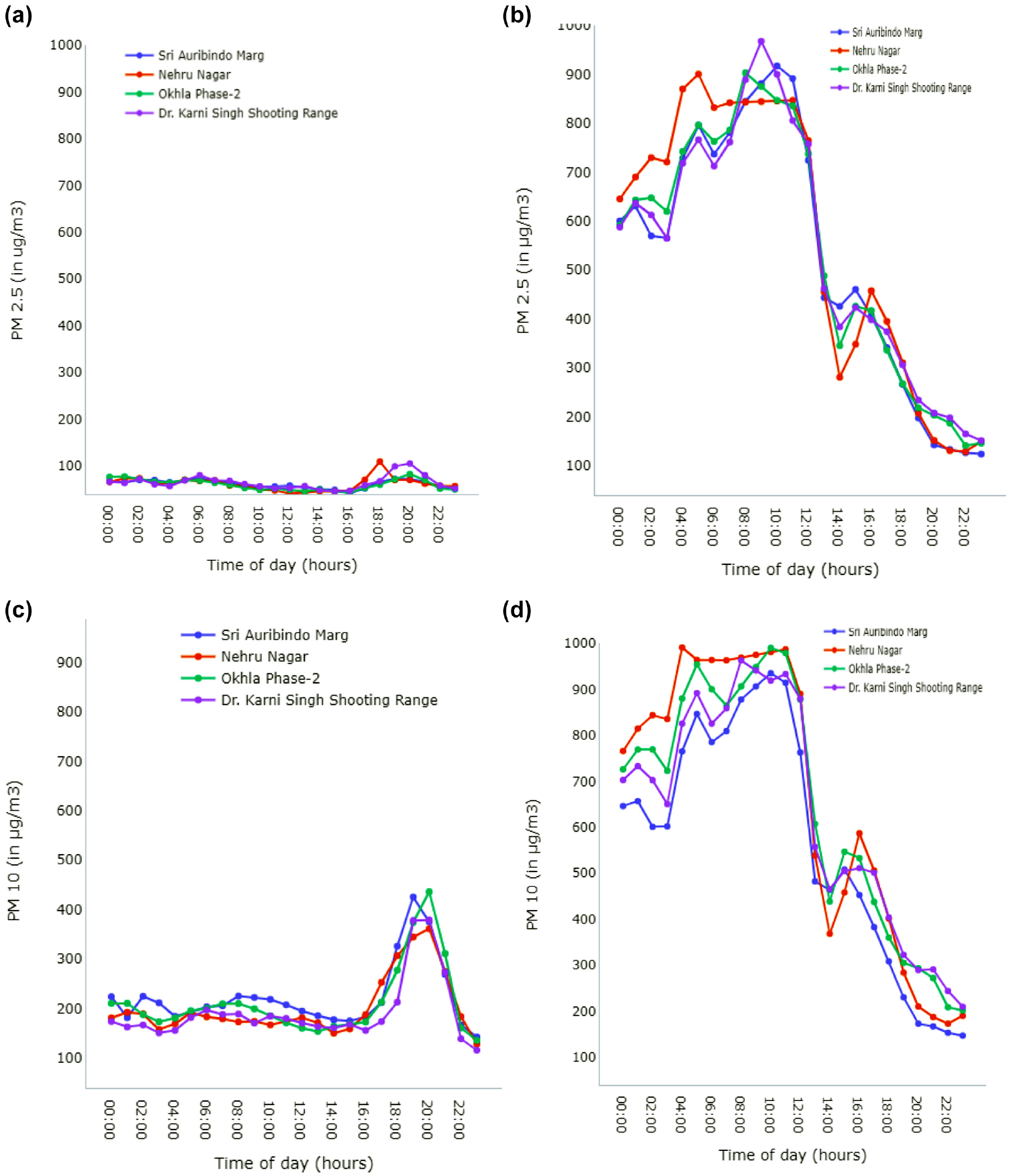
Seasonal variation of PM2.5 and PM10 for June 5, 2019 (left) and November 3, 2019 (right): (a) PM2.5, June 5, 2019, (b) PM2.5, November 3, 2019, (c) PM10, June 5, 2019, and (d) PM10, November 3, 2019.

Study Area

The majority of Indian cities suffer from extremely high levels of urban air pollution, particularly in the form of small-sized particulate matter ( 5 , 32 ). According to the World Health Organization (WHO), the capital city of India, Delhi, is one of the most polluted cities in the world ( 5 ). Pollution in Delhi usually spikes during the winter. For instance, it exceeded almost 40 times the WHO’s ambient concentration limits in the first week of November 2019 for PM2.5, that is, a concentration value of around 950 μg/m³ ( 33 ). Delhi is divided into 11 districts, out of which the South Delhi district has the highest number of static monitors for its area. There are four monitors in the South Delhi district for which the data is collected from the CPCB. The available static monitors in the area are located at Dr. Karni Singh Shooting Range, Nehru Nagar, Okhla Phase-2, and Sri Aurobindo Marg, and are all deployed by Delhi Pollution Control Committee (DPCC) authority (see Figure 2).

OPEN IN VIEWER

Figure 2.

Hexagonal grids and static monitors in South Delhi.

The data should belong to monitors closer to the location where prediction is to be made to get better prediction. Ideally, this would mean having a dense monitoring network. A model trained with the more extensive urban agglomeration area data is less likely to be accurate than multiple models trained with the data from localized, multiple, smaller zones. Further, in a dynamic monitoring network, having data from the same point is not possible, as data will be distributed over space and time. Therefore, the cells are created, and models are developed for each cell by converging the data points at the centroid of the cell. In spatial analysis, grids of points or polygons are frequently used to sample, index, or partition an area. The square and triangular shapes are commonly employed in the grid designs because of their simplicity in the definition, data storage, and ease of re-sampling to different spatial scales. Although hexagonal grids are not very common, these are becoming more popular, with hexagonal grids being a better approximation of the human vision grid ( 34 ). In the past, many studies used hexagonal grids for spatial visualization, and analysis ( 35 ). Regular hexagons feature additional symmetries and are the closest form to the circle, so they are more appropriate for spatial data sets that suit this study perfectly. Hexagons are better at fitting the earth’s curvature than squares when dealing with a large spatial area where the globe’s curvature becomes essential. Therefore, hexagonal grids of 5 km side-to-side spacing covering the whole area of South Delhi are adopted for the current study, as shown in Figure 2. With this, there are a total of 15 cells in South Delhi (see Figure 2), for which the prediction models are developed.

Data Set Formation

The detailed process of flow of this paper is shown in Figure 3. The first part is to select the study area and collect the hourly data set of static monitors in South Delhi. The next step is to generate augmented data sets using various interpolation techniques like IDW and Kriging, followed by preprocessing the data, including interpolating the null values, normalizing the data, and converting the data into a sliding window technique. Further, the data set is divided into training, validation, and testing sets. Then, various deep-learning models, such as CNN, LSTM, and CNN-LSTM, are developed for model prediction. Mean absolute error (MAE) and root mean square error (RMSE) are used for comparing the model’s accuracy.

OPEN IN VIEWER

Figure 3.

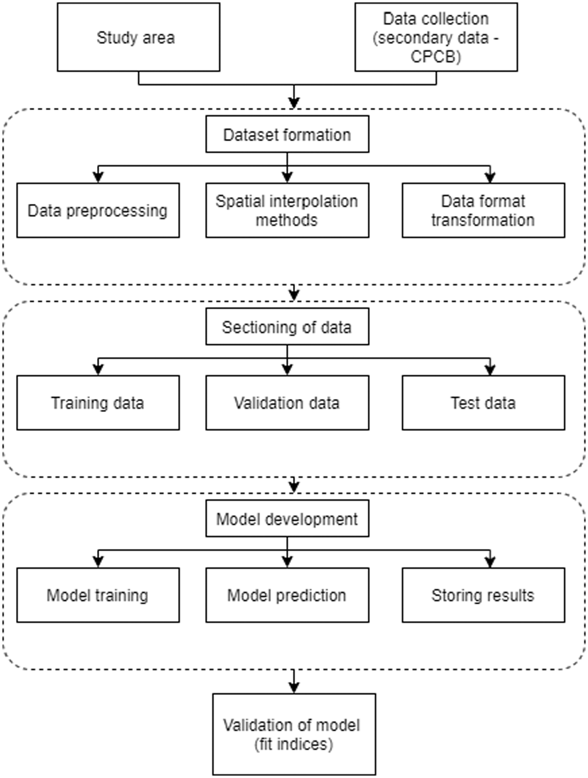
Methodology for the prediction modeling.

Data Preprocessing

Preprocessing of data is performed to address the noise in the data, missing values, and other erroneous variables in the collected data to develop a robust prediction model. In machine-learning models, data preprocessing refers to converting the raw data into readable input for the machine-learning model. There were missing values in the air quality data, and the reason could have been sensor device failure or network issues in data storing. Null values in a data set can lead to inaccurate results or failure of the model itself. The null values are replaced with mean values of the previous hour and following-hour values to eliminate the errors in the model that can occur because of missing values.

Normalization

Normalization gives equal importance to each parameter so that no single variable controls model performance in one direction just because it is greater in absolute terms. Normalization of the data set can also help in boosting the training speed and improving prediction accuracy. Also, variables assessed at different scales may not contribute equally to the model fitting, which might lead to bias, so the data set is normalized between 0 and 1 using Equation 1.

X ′ = X i − X min X max − X min

(1)

where X i is the original sample value, X max and X min are the maximum and minimum value of the whole parameter of original data, and X ′ is the value after normalization.

Correlation

Understanding the relationship between the parameters is essential while studying the machine-learning model data set. Figure 4 displays Pearson’s correlation heatmap for different parameters in the data set. The Pearson’s correlation ranges from −1 to 1, where the absolute value shows the intensity of correlation (1 being highest, 0 being lowest), and the sign shows the direction (positive or negative). A correlation value close to zero indicates the independence and absence of a relationship between the parameters. In Figure 4, higher correlation values are represented as dark green/red panels.

OPEN IN VIEWER

Figure 4.

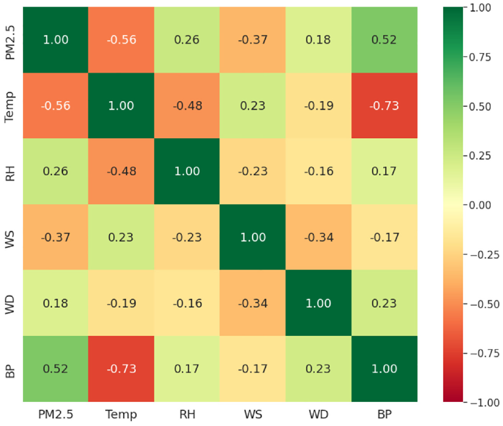
Correlation between input parameters of the model.

For PM2.5, a negative correlation is observed with temperature and wind speed, which indicates that with the increase in temperature or wind speed, the PM2.5 concentration will decrease. It can also be verified with Figure 1, which shows a lower concentration of PM2.5 in summers than in winters. A positive correlation of PM2.5 with barometric pressure and relative humidity is observed, which shows that with an increase in pressure and humidity, the concentration of particulate matter also increases. There are no parameters with exceptionally strong correlation. Therefore, all the parameters are considered for further modeling.

Spatial Interpolation Techniques

After the hexagonal grid formation for dividing the study area into smaller spatial regions, the data point for each cell is fixed as the centroid of each hexagon, respectively. Several spatial interpolation methods were used widely in past studies, such as IDW, Kriging, spline, Thiessen polygon, kernel density estimation, and so forth ( 36 ). There is no rule of thumb for the selection of interpolation methods. Two of the available spatial interpolation techniques are widely used and, thus, employed to generate the data set at each centroid for grids. Figure 5 explains the steps followed for the creation of an augmented data set for each cell. Initially, the raw data from four static monitors in South Delhi is collected from CPCB. Then the centroids of all the cells are located. The IDW method is used to determine the pollutant concentrations (PM2.5 and PM10) at centroids of the hexagonal cells, and the ordinary 2D Kriging method is employed for the spatial prediction of meteorological parameters such as relative humidity and barometric pressure.

OPEN IN VIEWER

Figure 5.

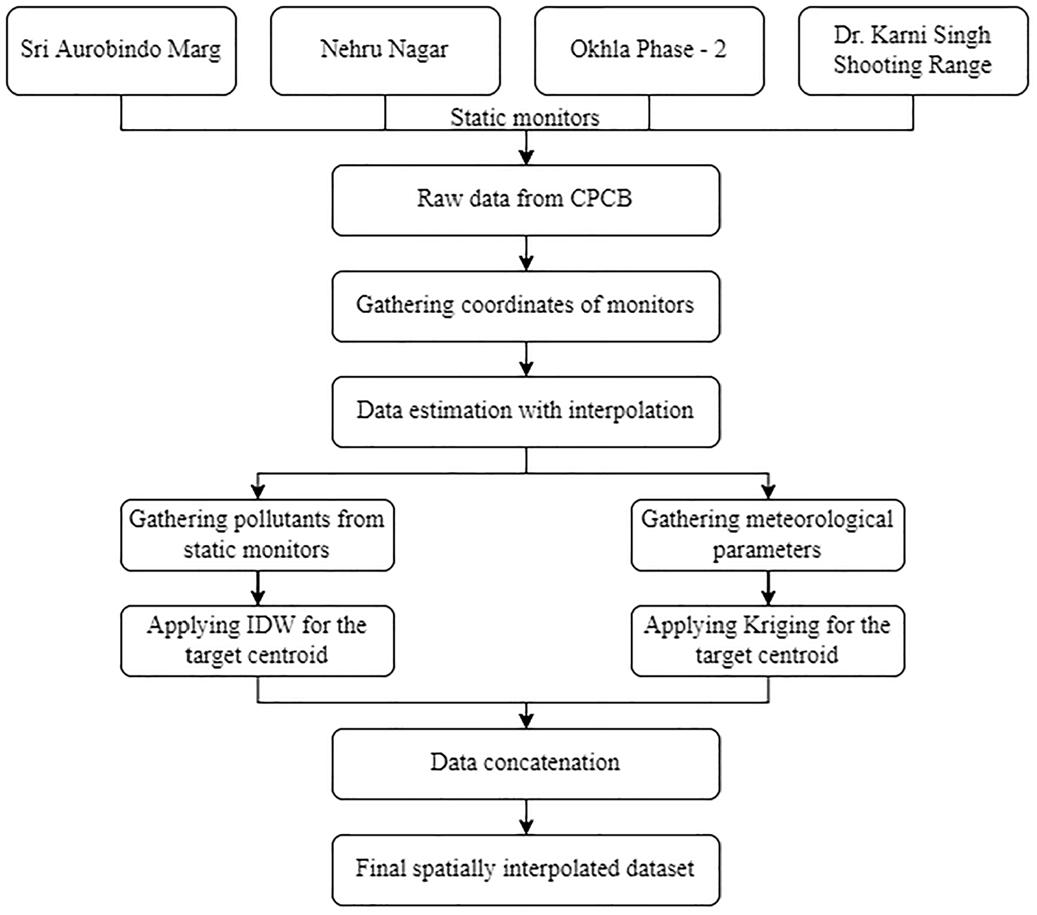
Augmented data set creation.

In addition to the data from static monitors, the different data points from the dynamic monitoring networks within a grid will be collated using IDW and 2D Kriging to the centroid of the grids, as explained in the following sections. The results from both methods are concatenated at the end to form a single data set for each cell.

Inverse Distance Weighting (IDW)

In IDW, the known points are locations where data is directly measured from monitors, and the determined values (from interpolation) depend on the distance between known and unknown points. The controlling power of the influence can be externally defined for a smooth resulting surface. Power of 2 is most commonly used in the literature ( 5 ) and therefore used in this study. The mathematical formula for IDW is given in Equation 2.

z j = ∑ i z i d ij n / ∑ i 1 d ij n

(2)

where z i is the value at a known point, d ij is the distance between the known and an unknown point, z j is the predicted value at the unknown point, and n is a user selected exponent (often 1, 2, or 3).

2D Kriging

The Kriging method of spatial interpolation is flexible to adopt different parameters and variogram forms and has a wide range of applications ( 36 ). In IDW, the weights are solely dependent on the distance, while in Kriging, the weights depend on the overall spatial arrangement of measured points and the distance between measured and prediction points. When IDW is applied for the spatial interpolation of meteorological parameters, the interpolated values for relative humidity and pressure are observed far from the actual value. Therefore the Kriging method is employed, which is more realistic. The equation for Kriging interpolation is shown in Equation 3. Kriging is a two-step process, it includes:

Creation of variograms and covariance to determine the spatial autocorrelation, and

Prediction of unknown values.

Different types of variograms, such as circular, spherical, Gaussian, exponential, and linear, can be used. Ordinary Kriging is widely used, with an assumption of unknown constant means. In this study, the PyKrige toolkit is used to perform ordinary 2D Kriging interpolation on the data set ( 37 ).

z j = ∑ i = 1 n λ i z i

(3)

where z i is the value at a known point, z j is the predicted value at an unknown point, λ i is a unique weight for location i , and n is a user selected exponent (often 1, 2, or 3).

Data Transformation

Data transformation refers to the process of converting raw data into data ready for modeling by removing unused columns, changing data types, altering the timestamps, and handling the errors in data. The factors which influence variables from time to time are determined through time-series models. While training the model, the results for a subsequent hour, from various sliding window sizes, are used, varying from 24 to 96 h, out of which 72 h is found to be the optimal value during the model formulation and experimentation. For this study the sliding window approach is adopted, whereby the data set of the period from January 2019 to April 2021 is divided into 72 h windows and 1 h strides.

This technique is followed for all the models to reshape the information using a fixed window so that the model is comprehensible for the complete information possible at a given period to achieve an accurate prediction.

Model Development

It is evident from exploratory data analysis that the pollutants and meteorological parameters highly influence one another. These parameters tend to follow specific trends and patterns that are extracted using deep neural networks specially designed for this task. In this study, three types of models are used, that is, CNN, LSTM, and CNN-LSTM, as discussed in the literature review.

Convolutional Neural Network

CNN models are mainly used for visual tasks but are not limited to these. Figure 6 shows the architecture for the CNN model, which is applied for prediction of PM2.5. CNN is used to capture various trends of pollutants and other meteorological parameters by treating the 72×7 matrix, which is created using a sliding window approach; a pattern is identified using CNN pattern recognition ( 38 ). Each convolution layer contains a series of filters known as kernels. A kernel is a matrix that moves over the input data, performs the dot product with the subregion of input data, and gets the output as the matrix of dot products, and each filter tries to learn a new trend in the previous hours. Through hyperparameter tuning of the CNN architecture model, the best parameters to the architecture are shown in Figure 6. The CNN architecture shown in Figure 6 uses a 3 × 3 kernel with 90 feature maps with stride set to 1 and padding set to SAME. Rectified linear unit (ReLU) is used as an activation function, which can solve the problem of gradient disappearance, and its calculation speed and convergence speed are faster than other activation functions ( 39 ). It is followed by a max-pooling layer of size 1 × 3, which reduces its resolution and complexity to achieve translation invariance. After that, there is a layer of batch normalization that helps deep neural networks to standardize the inputs to a layer for each mini-batch. This is followed with the same sequence of layers with 45 filters in convolution layer followed again with a max-pooling layer of size 1 × 3 and a batch normalization connecting to a dense network, using sigmoid in the end to predict the output. As a consequence of the normalized values, in range (0,1), the sigmoid function at the outer layer is logical. The sigmoid activation function is used in several previous studies for deep-learning models ( 22 , 23 ). At the last stage of the network, with the help of a flatten layer, the output from the batch normalization layer is fed into a fully connected dense layer that is reshaped into 9720 neurons (45 × 72 × 3), and seven parameters are predicted, including the pollutant concentrations and the meteorological parameters.

OPEN IN VIEWER

Figure 6.

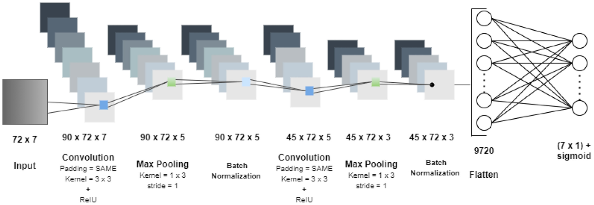
Architecture for convolutional neural network (CNN) model.

Long Short-Term Memory

LSTM is a variant of the traditional neural networks that exhibit dynamic behavior. It helps the network capture the data’s context for various operations, especially time-series forecasting. Since LSTM models are generally used for sequential analysis and have the capability of long-term dependencies, they can be trained to predict all the parameters for air quality for the next hour by the historical data gathered for various grids. The proposed system is trained with the data set at the centroid for each cell, shown in Figure 2.

A four-layer LSTM architecture is employed for the current study. A 72 × 7 matrix data layer is used for the input, which depicts the data for 72 h and seven parameters. Hyperparameter tuning is performed to get good prediction model architecture on LSTM architecture by working with different LSTM cells and layers and using the best prediction architecture as shown in Figure 7. The first two LSTM layers have 80 and 50 LSTM cells, respectively, with a dropout layer of 25%. This manages to stop all LSTM cells in a layer from synchronously optimizing their weights, thus helping the model avoid overfitting conditions. Then the following layers are supported by one more LSTM layer with 25 cells followed by a fully connected layer and output neural network layer with activation function as sigmoid as shown in Figure 7.

OPEN IN VIEWER

Figure 7.

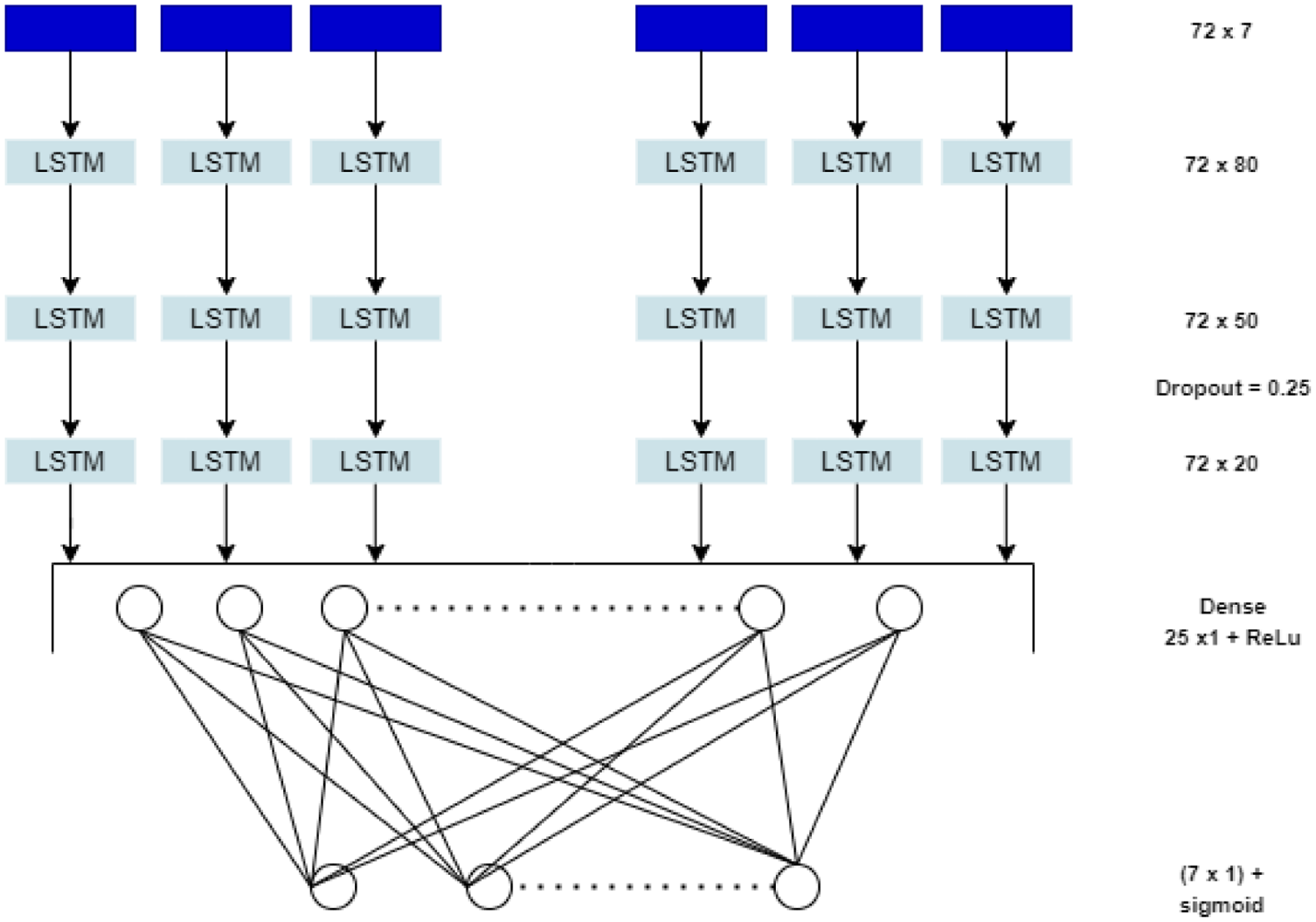
Architecture for long short-term memory (LSTM) model.

CNN-LSTM Model

The present study also proposes a hybrid CNN-LSTM model, which combines the time-series model of LSTM with CNN to extract effective features from data. The architecture of the proposed CNN-LSTM is shown in Figure 8. The inputs of CNN-LSTM are the tensors of the PM concentrations and meteorological parameters over the last 72 h. The output is received as prediction for all the input data parameters for the next hour. Unlike regular CNN or LSTM architectures, the first half of the architecture is CNN and is used for feature extraction. The following half of the architecture is LSTM forecasting, which analyzes the features extracted by CNN and then estimates the PM concentrations and meteorological parameters. Moreover, to improve the accuracy, additional batch normalization and dropout layers are added to the architecture of CNN-LSTM.

OPEN IN VIEWER

Figure 8.

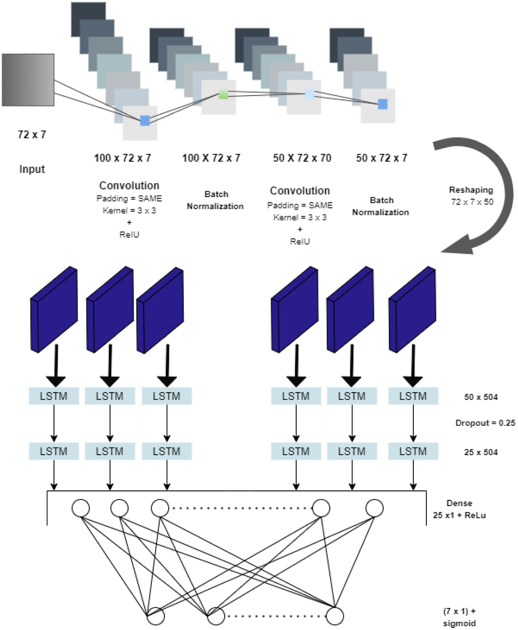
Architecture for CNN-LSTM model.

CNN is utilized for feature extraction; specifically, two two-dimensional convolution layers and two batch normalization layers are constructed. To prepare the data and put it into the format required by the LSTM, a reshape layer is connected to the LSTM; this is a layer that reshapes inputs into the given shape. As the various filter maps contain the reoccurring patterns and features now, they feed to the LSTM. There are two LSTM layers and in between a dropout layer to avoid overfitting, which is a common aspect in neural networks, and there are many solutions available. Among all of them, dropout is one of the efficient ones. Therefore, a dropout layer is added, the output of which is connected to the LSTM layer for prediction and finally joined to a fully connected layer and an output layer as shown in Figure 8. The CNN part of the CNN-LSTM architecture used in this study comprises two convolutional layers of size 100 and 50, respectively; that is, the first convolution layer has 100 unique feature maps used to extract the various trends and the second convolution layer has 50 unique feature maps. Each of the convolution layers is followed by a batch normalization layer which solves the issue of internal covariate shift ( 40 ). The output from the second batch normalized layer is reshaped to feed it as the input to the LSTM layer, and there are 50 units in the first LSTM layer, which are followed by a dropout of 0.25 that prevents neural networks from overfitting ( 41 ). Finally, one more LSTM layer is added of 25 units, followed by a fully connected dense layer that gives final output using sigmoid as an output function.

Results and Discussions

This study explores deep-learning techniques for spatiotemporal prediction of particulate matter and meteorological parameters. For this, three deep-learning models are developed for the temporal prediction of PM2.5, which provides an understanding of the trends and prediction for particulate matters over a selected region of Delhi. For the development of the deep-learning models, Google Colab platform is used ( 42 ). Each of the models is trained with 30 epochs. The configuration includes 2vCPU, 12 GB RAM, and GPU performances of 4.1 and 8.1 TFLOPS for Tesla K80 and T4 GPUs. Average training time per epoch is observed as 3 s for CNN, 6 s for LSTM, and 16 s for the proposed CNN-LSTM model. With increasing complexity the computational burden of the model also increases.

One of the static monitors is at the centroid of cell K; therefore, the actual data is available for this cell and used for sanity testing. The actual values are the PM2.5 concentration data from the static monitor. In contrast, the interpolated values are obtained from applying IDW on data from all four static monitors and estimating the values at the centroid of a cell. As proposed in the present study, the data from mobile monitoring networks would be aggregated to these cells. Since the dynamic monitoring network was not deployed, no historical data was available. Because of the COVID-19 pandemic, the portable devices could not be deployed and test data is also imputed from the static monitors.

To evaluate and compare the accuracy of the deep-learning models for PM2.5 predictions using the input data, the RMSE and MAE values are used. Evaluation parameters such as RMSE and MAE explain the performance of deep-learning models developed for forecasting. These can be used to achieve the desired accuracy of models. MAE (Equation 4) measures the average magnitude of the errors of the predictions without considering their direction by taking modulus. It is an average over the test sample of the absolute differences between predicted and actual observations where all individual differences have equal weight. Similarly, RMSE (Equation 5) follows the quadratic scoring rule that also measures the average magnitude of the error. It is the square root of the average of squared differences between predicted and actual observation, and it allows us to estimate the standard deviation ( σ ) of the error for a typical single observation.

The MAE and RMSE are given by Equations 4 and 5.

MAE = ∑ i = 1 n | x i − y i | n

(4)

RMSE = ∑ i = 1 n ( x i − y i ) 2 n

(5)

where x i is the estimated time series, y i is the actual observations time series, and n is the number of non-missing data points.

Figure 9 shows the MAE in each model for all cells, and it can be observed that the MAE value for the CNN-LSTM model is less than the MAE value for CNN and LSTM models for the majority of cells. Similar to MAE values, Figure 10 shows the RMSE values of each model for all grids. A similar trend is followed that shows only three out of 15 grids with RMSE value for the CNN-LSTM model have higher RMSE value than at least one of the other two models.

OPEN IN VIEWER

Figure 9.

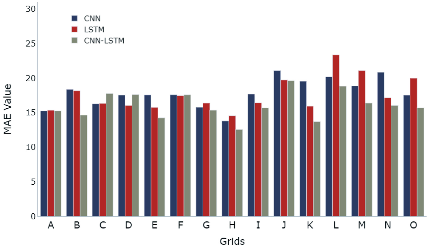
Mean absolute error (MAE) in each model for all grids.

OPEN IN VIEWER

Figure 10.

Root mean square error (RMSE) in each model for all grids.

The comparative results and evaluation of the models confirm that the combined model of CNN-LSTM outperforms CNN and LSTM models for 10 cells out of a total of 15 cells. Further, the predicted value is compared with the actual value for all three models.

Figures 11 to 13 show the difference between predicted and actual values of PM2.5 over the duration of 360 h from April 15 to 30, 2021, for the CNN, CNN-LSTM, and LSTM model for cells H, L, and N. Along with confirmation from MAE and RMSE values about CNN-LSTM being the most suitable model (Figures 9 and 10), Figures 11c, 12c, and 13c also show that the curve for actual and predicted values of PM2.5 has minimum deviations for the CNN-LSTM model.

OPEN IN VIEWER

Figure 11.

The results of: CNN (a), LSTM (b), and CNN-LSTM (c) for grid H.

OPEN IN VIEWER

Figure 12.

The results of: CNN (a), LSTM (b), and CNN-LSTM (c) for grid L.

OPEN IN VIEWER

Figure 13.

The results of: (a) CNN, (b) LSTM, and (c) CNN-LSTM for grid N.

For determining the model accuracy, hourly PM2.5 concentrations data for 2 months from May 1 to June 30, 2021, is collected for four static monitors from CPCB. For the centroid of each cell, the data is interpolated using IDW and Kriging. As shown in Figure 2, one of the static monitors located at Dr. Karni Singh Shooting Range lies in grid K. Therefore, to compare the actual values obtained from the static monitor and predicted values estimated from models, grid K is selected. Figure 14 compares the actual (data from static monitors) and predicted values of PM2.5 using the three deep-learning techniques, CNN, LSTM, and CNN-LSTM. It confirms that the CNN-LSTM can predict the PM2.5 efficiently.

OPEN IN VIEWER

Figure 14.

Results of CNN (top), LSTM (middle), and CNN-LSTM (bottom) for cell K, for time period from May 1, 2021 to June 30, 2021.

The present study shows that the results for CNN-LSTM along with the individual models of CNN and LSTM, presented for 360 h in Figures 11 to 13, are better than the results shown in the literature ( 21 ), where the results for CNN and LSTM individually were explained for the next 8 h time span. A CNN-LSTM model was developed without batch normalization, which is a very crucial step to solve the problem of internal covariate shift; the model also used one-dimensional CNN layers that limit the motion of kernel to one direction only and limit the full strength of CNN-LSTM ( 23 ). In contrast, the current study uses two-dimensional CNN layers to improve the strength of CNN-LSTM models. It is found that temperature is highly correlated to PM2.5 trends (Figures 1 and 4), while the influence of temperature was not considered for PM2.5 prediction using a similar model of CNN-LSTM ( 22 ).

Figure 15 depicts the spatial prediction at the centroid of each cell using the CNN-LSTM model in peak (08:00) and off-peak (15:00) hours for February 1, 2021 and June 28, 2021, respectively. First, as expected, the winter (Figure 15a) and summer (Figure 15b) seasons have significant differences in PM2.5. Interestingly, a major difference can be observed within South Delhi depending on the cell location and time of the day, that is, road users may get a chance to alter the choice (e.g., route and departure time) and reduce their air pollution exposure. The accuracy of the model can be further enhanced by using the dynamic monitoring network.

OPEN IN VIEWER

Figure 15.

Spatial prediction of PM2.5 from CNN-LSTM for February 1, 2021 and June 28, 2021 in peak hour (left) and off-peak hour (right): (a) February 1, 2021, 08:00 (peak hour, left) and 15:00 (off peak, right), and (b) June 28, 2021, 08:00 (peak hour, left) and 15:00 (off peak, right).

The practical applications of this study lie in estimating the accurate PM concentrations for researchers, policymakers, officials related to the environment, and the public. The commuters in Delhi are willing to update their travel choices provided air pollution and route information is provided to them ( 43 ). Commuters can consider the pollution levels in changing their travel behavior, such as changing the travel mode, changing the departure time, choosing to travel or staying at home, and so forth. The different route possibilities (e.g., shortest path, greenest path, balanced path, etc.) would facilitate the commuters to reduce their air pollution exposure based on real-time congestion and air pollution patterns ( 44 ). In the long run, residence selection (e.g., location choice) can also depend on the levels of air pollution in different areas. This indicates that with the help of a prediction framework, a provision for disseminating air pollution information can be provided, which is likely to reduce the air pollution exposure of daily commuters.

Conclusions

To understand dynamic air pollution and push people to make informed decisions and prevent health issues arising from increasing air pollution, providing information on all routes is essential. People face maximum exposure to air pollution while traveling. Therefore, travel choices such as travel mode and route influence the exposure and have an extremely strong effect on human health. For estimating exposure on all commuter routes, the concentration of pollutants at each point in the vicinity is required. Because of cost factors, the monitor network cannot be dense enough to provide accurate values at each location. For determining pollutant concentration on all routes, high-resolution spatial prediction and accurate forecasting are required. This paper proposed a framework for the development of a prediction model for PM2.5 pollutants in the South Delhi region of India. The model is applicable for a dynamic monitoring network. Historical data was collected from CPCB for all meteorological parameters and particulate matters of four static monitors from South Delhi

Initially, the model was developed through two techniques, that is, CNN and LSTM, on the meteorological parameters of temperature, relative humidity, pressure, wind speed and direction, and particulate matter. The prediction model inputs the previous 72 h data and predicts the following-hour data of particulate matter and other meteorological parameters. A hybrid model was proposed as a combination of CNN and LSTM, whereby CNN extracts the effective features and LSTM manages time-series data processing to improve the accuracy of the prediction model. Through experimental results, we found that the CNN-LSTM model outperforms the remaining models. The proposed model may provide abrupt predictions if external environmental factors like a sudden increase in toxic gases and traffic congestion are present. As the unknown causes of change in pollution concentrations cannot be added in models, this limitation exists. Because of the pandemic situation, portable monitors could not be deployed, and thus the data from dynamic monitoring networks is not part of the results. However, the dynamic data from mobile monitors can be accommodated in the proposed framework, which is likely to further improve the model’s accuracy. This study shows the proof of concept for providing a prediction framework for dynamic air pollution and meteorological data, in which a grid size of 5 km is assumed. A smaller grid size will increase the number of models and thus the requirement of computational efforts but may also increase the spatial accuracy ( 45 ).

In the future, the authors wish to utilize the data from the dynamic monitors for the prediction framework, exploit a way to reduce the need for a model for each grid, and implement a concept of hybrid grid sizes for the dynamic data. Since the framework is transferable, planners and practitioners can employ the same models in different cities and use the predicted values to provide green travel routes.