Clustering-Based Travel Pattern for Individual Travel Prediction of Frequent Passengers by Using Transit Smart Card

Abstract

Individual travel prediction is very important for the construction of intelligent urban transportation systems. Previous studies mainly focus on the improvement of algorithms, but pay little attention to the mining of data information. In this paper, the concept of the travel pattern is introduced into the field of individual travel prediction of frequent bus passengers. The travel pattern of passengers refers to the trip with similar boarding time and similar boarding and alighting stations of the same person. Through clustering the travel pattern by DBSCAN algorithm, the regularity of passenger travel can be better exploited and travel information can be integrated into a unified unit as well. In the process of prediction, we first predict whether the passenger will travel, and then, if so, predict the probability distribution of the next trip conditional on the previous one. The proposed method is tested using the Automatic Fare Collection data of Chengdu’s frequent bus passengers in May 2019. Based on travel pattern, the average accuracy of travel information prediction is about 41%, which is 13% higher than the method without using travel pattern. Furthermore, this paper also discusses the influence of spatial threshold in clustering on the prediction results.

Keywords

Data and data science AVL data origin and destination data planning and analysis pattern (behavior choices etc.)public transportation buses

Individual travel prediction is based on a disaggregate model, which takes the differences between individual trips of passengers into account. Compared with group research using the aggregate model, individual travel prediction aims to provide personalized services for passengers. Nowadays, with the concept of MaaS (Mobility as a Service) being further popularized, the prediction of individual demand is more and more important. Furthermore, individual travel prediction is also one of the key factors to support various applications of the intelligent traffic system, such as personalized traveler information, targeted demand management, and dynamic system operation, which can effectively improve the customer experience and the performance of the traffic system (1).

In regard to prediction content, previous studies mainly focused on the location that the user will visit next ( 2 ) or the location of the user in the next timestamp (often set as an hour) ( 3 ). In this kind of problem, the prediction accuracy tends to be higher when people have lower travel frequency ( 3 ). However, in transportation, we pay more attention to the few hours when people travel ( 1 ). Therefore Zhao et al. ( 1 ) take next trip as the prediction object and trip information as the prediction content to predict whether passengers will travel and attributes of the next trip, which are composed of trip start time T, origin O, and destination D. They predicted the three travel attributes respectively according to the order of T, O, D, and the real values of T and O are used to predict the following travel attributes. However, this method is meaningless in reality, for the real O can be obtained while getting the real T in the public transport system. In this paper, we will predict all the travel attributes at the same time because of the strong correlation between spatial and temporal attributes in travel, which is a key point that has never been noticed in the previous literature.

In regard to data sources, the most commonly used data set is mobile phone data ( 2 ); in addition, there are Wi-Fi data ( 4 ), global positioning system (GPS) data ( 5 ), and so on. These kinds of data are generated by non-transportation activities, and cannot be interpreted as travel behavior directly ( 1 ). Generally, the information we can get from such data is the location of the user at regular intervals (depending on the collection time interval of the device), whereas the start time, origin, and destination of each trip cannot be obtained directly. And, it is difficult to convert such data into travel behavior because of the correlated but distinct personal preferences which vary across individuals (6). Another kind of data is collected from urban transportation systems, such as the transit smart card data ( 7 – 9 ) adopted in this paper. This kind of data is obtained by individual travel decisions, including the start and end stations of the travel and the corresponding timestamp. Thus, transit smart card data can be used to predict the next trip in real time according to the passenger’s travel decision, which is also very important because the demand of the individual is time sensitive.

Although several algorithms have been proposed for individual travel prediction, there is no existing model for the prediction of all of the travel attributes of the next trip at the same time. Previous studies mainly focus on the improvement of algorithms, but pay little attention to the mining of data information. Most of them only describe the phenomenon of travel, or summarize some travel rules in some aggregate methods, but lack mining the historical travel rules of individual passengers. Therefore, this paper introduces the concept of the individual travel pattern (which will be discussed in next section) into the field of individual travel prediction, and establishes a real-time prediction model for all of the travel attributes of the next trip of the individual passenger. The result of whether to use the travel pattern for prediction will also be compared by using the IC card data of Chengdu, China in this paper.

The rest of this paper is organized as follows. The second section reviews the literature related to this paper. The third section covers the data set and the preparation of data. The fourth section introduces the clustering method of travel patterns and the algorithm of individual travel prediction based on travel patterns. The fifth section will use Chengdu’s IC card data to evaluate the effects of algorithm.

The influence of spatial threshold in clustering on the prediction results is discussed in the sixth section. Finally, the conclusion of this paper is given.

Literature Review

Most existing methods for individual mobility prediction are based on modeling sequential patterns of individual location histories, and the most common way is to model the location sequence by Markov chain (MC). Lu et al. proved that even the simple MC model can achieve high prediction performance in the question of next location prediction ( 10 ). Gambs et al. proposed a mobility Markov chain to discuss the influence of the previous k locations on the prediction results, and they found that the accuracy of predicting the next location can reach 70–95% when k = 2 ( 11 ). And when k increases, the prediction result will not improve much, but it will lead to calculation difficulty caused by the increase of the number of transition probabilities. This kind of research only considers the spatial attribute of travel and ignores the temporal attribute of travel. Alvarez-Lozano et al. used a hidden Markov model to propose a spatio-temporal prediction approach to forecast user location in a medium-term period (0.5 h–7 h) which considers that the users may have a different mobility pattern for each day of the week ( 12 ). However, they still did not match the travel time and location together.

From Table 1, it can be found that the aforementioned methods mainly focus on the next location prediction problem. In this paper, we focus on the problem of next trip prediction, which includes spatial and temporal attributes together. Zhao et al. proposed a Bayesian-based n-gram model, which divides the travel prediction into two parts: whether to travel or not and next trip attributes ( 1 ), and divides the trip into the first trip of the day and other trips. Compared with the MC method, the prediction of T (travel time), O (boarding station), and D (alighting station) is improved by 10.6%, 7.5%, and 10.2%, respectively. Although the model can predict individual travel information, it still separates T, O, and D, which means that the prediction results of T and the first trip information of the day are not good. And when TOD is combined to predict together, the prediction accuracy of the first trip of the day and other trips are only 23% and 29.4%. The above methods all directly use individual historical travel data without mining potential information such as patterns and rules in personal travel history. In the vehicle trajectory prediction, Wang et al. used the method of segmented trajectory clustering to predict the destination of the vehicle ( 13 ). It segmented the sub-trajectories through the Douglas–Peucker-based algorithm for clustering the sub-trajectories, and then used the neural network method to predict the destination of the vehicle. This method achieved better results by using the historical regularity information of the vehicle compared with the method based on MC. However, this method of clustering passengers’ travel regularity before prediction has not been adopted in the field of bus passenger so far.

Table 1.

Summary of Existing Studies of Mobility Prediction

Research	Data	Method	Real-time prediction or not	Consider complete travel attributes or not	Prediction content and accuracy
Lu et al. ( 10 )	Mobile phone	Markov chain	No	No	Next location: 88%
Gambs et al. ( 11 )	GPS	Mobility Markov chain	No	No	Next location: 75%–90%
Sapiezynski et al. ( 4 )	WiFi	Side-channel location tracking	Yes	No	Location tracking: 80%
Alvarez-Lozano et al. ( 12 )	Mobile phone	Hidden Markov chain	No	No	Next period location: 30 min: 81.75%, 7 h: 66.25%
Zhao et al. ( 1 )	Transit smart card	Markov chain	Yes	Yes	Next trip: start time T: 31.5%, origin O: 70.8%, destination D: 55.3%, combination of TOD: 17.6%
Zhao et al. ( 1 )	Transit smart card	n-gram	Yes	Yes	Next trip: T: 42.1%, O: 78.3%, D: 65.5%, TOD: 29.4%

IC card data have the characteristics of large data volume, wide coverage, and high authenticity. In addition, because of the immutability of the passenger ID, long-term travel data for the same passenger can be obtained, which provides the possibility of mining the travel patterns of passengers and predicting the travel of passengers. The concept of travel pattern, which refers to the trip with similar boarding time and similar boarding and alighting stations, is usually used in the study of the regularity of bus passengers. Zhong et al. identified the quasi-periodicity of transit behavior ( 14 ); Goulet-Langlois et al. concluded that the sequence of travel events is an important part of travel pattern ( 9 ); Medina used a week’s IC card data and 1% of the residents’ travel survey data to obtain the main activity patterns of passengers ( 15 ). Through the study of travel pattern, it can be found that the travel of bus passengers is implied imply with regularity. Unfortunately, these findings about travel patterns have not yet been applied to bus passenger travel predictions.

In summary, the previous study of individual travel prediction has mainly focused on the improvement of methods, and MC or Bayesian distribution are mainly used to predict one single attribute of passenger travel or different travel attributes separately. However, the mining of spatio-temporal regularity which may be hidden in the individual travel data is missing. In regard to vehicle trajectory prediction, some scholars have begun to use the trajectory clustering method for prediction, and have achieved better results. For bus passengers, several studies have shown that their travel is associated with regularity, and the travel patterns of passengers can be obtained through clustering. Therefore, the use of travel pattern in travel prediction is applicable to bus passengers. At the same time, the travel pattern integrates travel information which is more in line with individual travel prediction.

Data Preparation

This paper takes the bus IC card data of Chengdu, China in May 2019 as an example. Chengdu has a complex bus network and many bus passengers, with about 700 bus lines and over 8,000 bus stations. As shown in Figure 1 below, Chengdu bus stations are very densely distributed. In the area within the Third Ring Road (the red area in the Figure 1), there are more than 2,500 stations within a 200-square-kilometer area. Such a high-density distribution of bus stations lays the foundation for citizens to use public transport to travel. According to the IC card data of Chengdu in May 2019, the number of cards is 4,519,735, and the number of trips is 96,065,229. The average number of daily trips on weekdays and weekends are 3,451,356 and 2,358,674. This shows that many Chengdu citizens use public transportation as a way of travel, which provides a realistic basis for the research in this paper.

Figure 1.

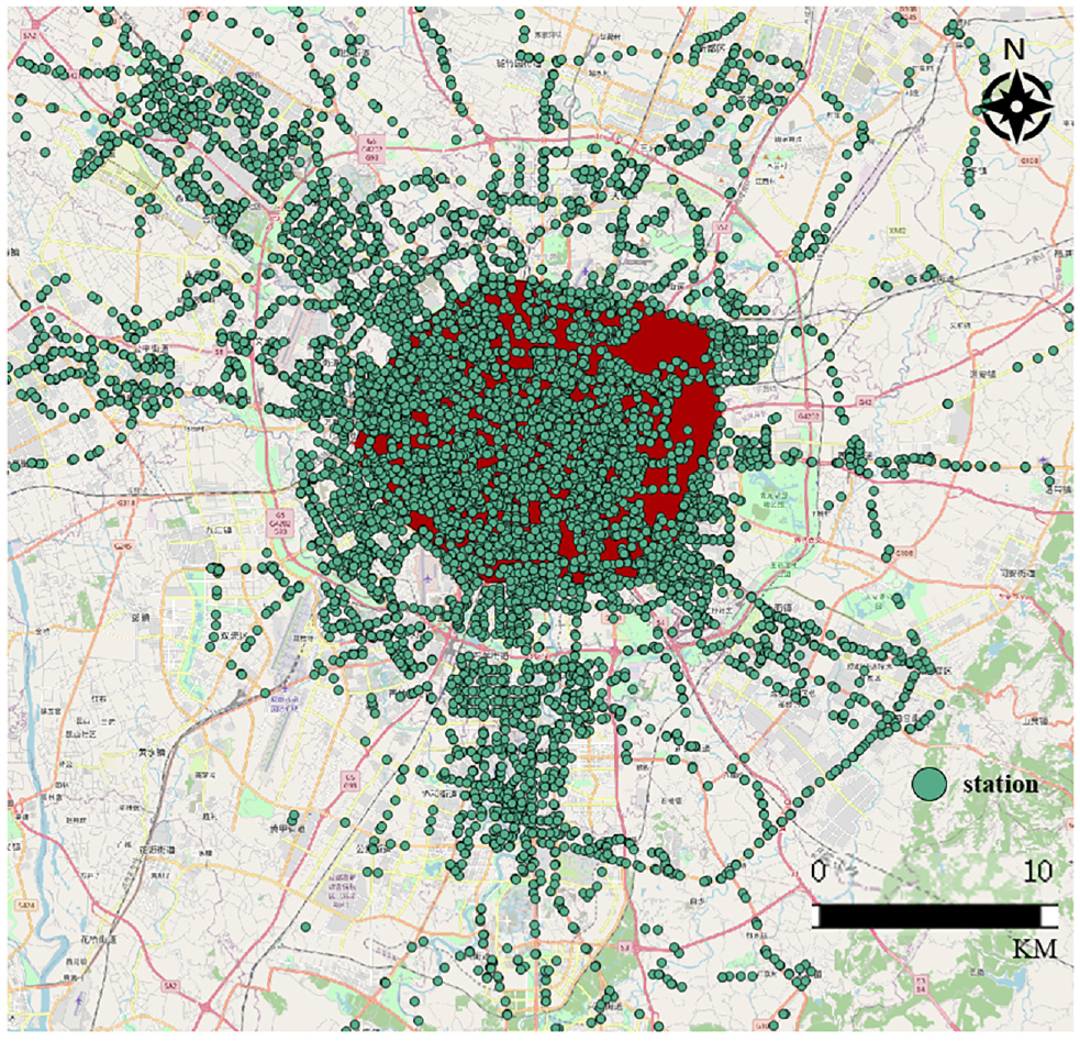
The map of bus station in Chengdu, China.

For Chengdu’s intelligent public transportation system, Automatic Fare Collection (AFC) data record information such as card number, card type, consume time, bus line ID, and vehicle ID; Automatic Vehicle Location (AVL) data record vehicle operation information for each bus; and Geographic Information System (GIS) data records the GPS information for each station. Through the fusion of GIS data and AVL data, the error records in GIS data will be corrected. Through the fusion of AFC and AVL data, the travel information of bus passengers can be inferred. The calculation of the boarding station is done mainly by matching the IC card and the GPS data of the bus, and selecting the location of the bus stop at the time of swiping the card as the boarding station. As passengers do not need to swipe their cards to get off, their alighting station needs to be inferred according to some assumptions. The two basic assumptions most commonly used are: (1) for two consecutive trips, the alighting station of the current trip is closest to the boarding station of the next trip; (2) the destination of the last trip of the day is the boarding station of the first trip of the previous day ( 16 – 18 ). For the identification of passenger transfer, this paper modified the two-stage transfer identification method of Nassir et al. ( 19 ) by using the actual walking distance obtained from Gaode map to replace the Euclidean distance between transfer stations. Finally, the calculated success rate of boarding station is 95.61%, and that of alighting station is 78.06%.

Among bus passengers, not only are there those who rely on public transport for most (or even all) travel, but also included are passengers who occasionally use public transport as a transfer method between different modes of transportation. Because the latter type of passengers use public transport less frequently and travel irregularly, in previous research scholars have usually deleted them from the research object by setting certain criteria. Zhao et al. selected passengers with more than 60 travel days and average trip rate over 1.99 per active day as the research object from 2 years of railway travel data in London ( 1 ); Goulet-Langlois et al. selected passengers with more than 10 trips in 1 week as the research object from 1 month’s London bus card data ( 9 ). In this paper, we used the travel frequency to filter the frequent bus passengers. This paper selects passengers who travel at least 60 times as the research object (travel at least twice a day on average). The problem of travel prediction for bus passengers with low-frequency trips is beyond the scope of this paper. After filtering, a total of 16,486,171 trips by 199,073 passengers entered the research dataset. Although only 4.4% of passengers were selected, these passengers made up 22% of all trips.

Methodology

Problem Formulation

The individual travel prediction studied in this paper is a dynamic prediction of passengers’ next travel information based on passengers’ historical travel pattern. People usually travel in days, so the prediction interval in this paper is 1 day (0:00–24:00). Dynamic prediction means that the real-time travel information of the passengers will be used to modify the last prediction result and continue to predict the next travel information under the revised results. Based on Zhao et al. ( 1 ), this paper divides travel prediction into the following four questions:

P1: Predict whether the passenger will travel on that day;

P2: Predict whether the passenger will make another trip based on the last trip observed;

P3: Predict the first travel information when the passenger will travel on that day (result of P1);

P4: Predict the next travel information when the passenger will make another trip (result of P2).

In this paper, we predict the passengers’ travel at the daily level, and exact the travel sequence by preserving the order of trips in the day. The travel sequence is represented as Equation 1. The $S^{u, v}$ is the travel sequence for passenger $u$ on day $v$ , and $k^{u, v}$ is the number of trips made by passenger $u$ on day $v$ , and the ( $t, o, d)$ refers to the start time, origin, and destination of the trip. For the convenience of calculation, the locations of the $o$ and $d$ are based on the GPS record of the station.

S^{u, v} = {(t_{1}^{u, v}, o_{1}^{u, v}, d_{1}^{u, v}), (t_{2}^{u, v}, o_{2}^{u, v}, d_{2}^{u, v}), \cdot \cdot \cdot \cdot, (t_{k^{u, v}}^{u, v}, o_{k^{u, v}}^{u, v}, d_{k^{u, v}}^{u, v})}

(1)

In this way, P1 and P2 can be convert to predict whether $k^{u, v}$ exists, and P3 and P4 can be convert to predict the $(t_{k^{u, v}}^{u, v}, o_{k^{u, v}}^{u, v}, d_{k^{u, v}}^{u, v})$ .

Algorithm of Individual Travel Prediction

The problem of P1 and P2 can be solved by a logistic regression model. For the problem of P3 and P4, we adopt the n-gram model which was introduced into the field of mobility prediction by Zhao et al. ( 1 ). The n-gram model is usually used to estimate the probability of different word sequences, and supports a series of applications such as speech recognition and machine translation. In this paper, the travel sequence $S^{u, v}$ can be treated as a sentence, and the unit of $(t_{k^{u, v}}^{u, v}, o_{k^{u, v}}^{u, v}, d_{k^{u, v}}^{u, v})$ can be treated as a word in the sentence.

The n-gram model is based on the following assumption: the occurrence of the nth word is only related to the previous (n–1) words and has nothing to do with other words. The probability of the whole sentence is the product of the probability of each word in the sentence. Suppose a sentence $S$ is composed of n words, such as, $S = w_{1} w_{2} w_{3} \dots w_{n}$ , and then the probability of its occurrence is expressed as Equation 2.

\begin{matrix} P (S) = P (w_{1}) P (w_{2} | w_{1}) P (w_{3} | w_{2} w_{1}) \cdot \cdot \cdot P (w_{n} | w_{1} \cdot \cdot \cdot w_{n - 1}) \end{matrix}

(2)

The $P (S)$ represents the probability that sentence $S$ appears in the data set, and $P (w_{n} | w_{1} \cdot \cdot \cdot w_{n - 1})$ represents the probability that the nth word of sentence $S$ is $w_{n}$ when the first (n–1) word is $w_{1} \cdot \cdot \cdot w_{n - 1}$ . Therefore, it can be seen that the generation probability of the nth word is determined by the first (n–1) words. But because of the length of the sentence is uncertain, the amount of calculation for the computer to calculate the probability distribution of the sentence will increase exponentially when the sentence is very long, which results in the inability to calculate the probability of the sentence. To solve this problem, the n-gram model defines that the word in the sentence is only related to its previous n words. When n = 2, it is called bigram model (2-gram model), and the corresponding $P (S)'$ is shown in Equation 3. According to Gambs et al. ( 11 ), it is sufficient to use the previous one location for the next location prediction. So, in this paper, the bigram model is adopted to solve P3 and P4.

\begin{matrix} P (S)' = Π_{i = 1}^{n} P (w_{i} | w_{i - 1}) \end{matrix}

(3)

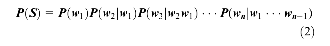
The probability value of $P (S)'$ can be solved by maximum likelihood estimation, which is shown in Equation 4. The $C (w_{i - 1} w_{i})$ means the counting number of $w_{i}$ in the case of $w_{i - 1}$ , and $C (w_{i - 1})$ means the counting number of $w_{i - 1}$ . For the discrete variable of time, the boarding time of any two trips is unlikely to be exactly the same. Therefore, to count accurately, this paper aggregates the time in an adjacent hour. The reason for selecting 1 hour is to correspond to the time threshold in the previous travel pattern. The n-gram model will face the sparse data problem when the training set is limited. To avoid the situation that the numerator and denominator are zero in Equation 4 as a result of a trip which has not occurred in the training set, Laplace smoothing is used. As shown in Equation 5, Laplacian smoothing forces each unit to appear at least once by adding one to the numerator and adding the number of units that have appeared in the data set ( $| V |)$ to the denominator.

\begin{matrix} P (w_{i} | w_{i - 1}) = \frac{C (w_{i - 1} w_{i})}{C (w_{i - 1})} \end{matrix}

(4)

\begin{matrix} P (w_{i} | w_{i - 1}) = \frac{C (w_{i - 1} w_{i}) + 1}{C (w_{i - 1}) + | V |} \end{matrix}

(5)

For the above four questions (P1–P4), we use the prediction method which is shown in Equations 6 –9, and it will be represented by TI in the following.

\begin{matrix} P 1 = P (y_{1} | F) \end{matrix}

(6)

\begin{matrix} P 2 = P (y_{i} | t_{i - 1}, o_{i - 1}, d_{i - 1}) \end{matrix}

(7)

\begin{matrix} P 3 = P (t_{1}, o_{1}, d_{1} | F) \end{matrix}

(8)

\begin{matrix} P 4 = P (t_{i}, o_{i}, d_{i} | t_{i - 1}, o_{i - 1}, d_{i - 1}) \end{matrix}

(9)

The $y_{1}$ and $y_{i}$ in $P 1$ and $P 2$ are binomial classification problems, which represent whether there will be the first trip and the $i^{th}$ trip. When predicting $P 1$ and $P 3$ , there is no travel record for that day because it is the first trip of the day, so we use the characteristics of the day ( $F$ ) to determine whether to travel and travel information. In this paper, we take the day of the week as the feature ( $F$ ) of the day.

Algorithm of Travel Pattern Identification

The direct use of travel attributes ( $t, o, d)$ for prediction not only leads to poor prediction results, but also leads to calculation difficulties because of the large number of possible combinations between ( $t_{i}, o_{i}, d_{i})$ and $(t_{i - 1}, o_{i - 1}, d_{i - 1})$ . Therefore, we explore the historical travel rules of passengers to reduce the number of possible combinations and improve the prediction results.

Through the research on bus passengers in previous literature ( 9 , 14 , 15 ), it can be found that some passenger trips have the same travel pattern, which means these kinds of trips have similar boarding time and similar boarding and alighting stations. Therefore, this paper introduces the concept of travel pattern into the prediction of individual travel. For the trips with travel patterns, we can establish the travel pattern sequence R of passengers based on Equation 1, and use the travel pattern M to replace the travel attributes ( $t, o, d)$ . The travel pattern sequence R is represented as Equation 10.

R^{u, v} = {(M_{1}^{u, v}), (M_{2}^{u, v}), \cdot \cdot \cdot \cdot, (M_{q^{u, v}}^{u, v})}

(10)

The $R^{u, v}$ is the travel pattern sequence for passenger $u$ on day $v$ , and $q^{u, v}$ is the number of travel patterns made by passenger $u$ on day $v$ .

The method of travel pattern identification in this paper is density-based spatial clustering algorithm with noise (DBSCAN). For IC card data, the greatest feature of DBSCAN algorithm is that there is no need to pre-determine the number of clusters, which is not available in other classical clustering algorithms (such as k-means, Gaussian mixture model, etc.). This feature is very important for the travel pattern because the number of individual travel patterns is unknown ( 20 ). Another clustering algorithm which also does not give the number of clusters in advance is the hierarchical method. However, it cannot be applied to large-scale data sets because of its low efficiency. The comparison of classical clustering algorithms is shown in Table 2. Therefore, DBSCAN algorithm is the most commonly method used in the study of travel pattern.

Table 2.

Comparison of Classical Clustering Algorithms

Algorithm category	Partition-based methods	Hierarchical methods	Model-based methods	Density-based methods
Representative algorithm	k-means	HAC	GMM	DBSCAN
Efficiency	Normal	Low	Normal	Normal
Noise resistance	Low	Normal	Normal	High
Is it necessary to give the number of clusters in advance	Yes	No	Yes	No

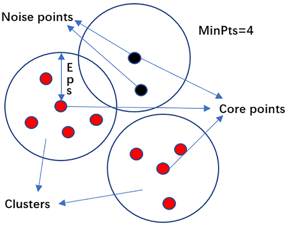
For the DBSCAN algorithm, there are two key parameters that need to be defined: radius distance ( $Eps$ ) and minimum number of points ( $MinPts$ ). The radius distance defines the reachable range of the density. If the distance between a sample and the core point is less than $Eps$ , the sample will be included in the cluster where the core point is located; $MinPts$ is the minimum number of records in each cluster. If the number of records in each cluster is less than $MinPts,$ these records are marked as noise. The principle of the algorithm is shown in Figure 2.

Figure 2.

Algorithm diagram of DBSCAN.

The travel pattern of passengers has three attributes: T, O, and D, so a dual-neighborhood DBSCAN algorithm is adopted in this paper, in which the neighborhood radius1 ( $Eps 1$ ) is the time distance between two trips, which is calculated by the difference of boarding time; neighborhood radius 2 ( $Eps 2$ ) is the spatial distance between two trips, and the spatial distance is calculated as Equation 11 shows:

D = \sqrt{{D_{1}}^{2} + {D_{2}}^{2}} * 1000

(11)

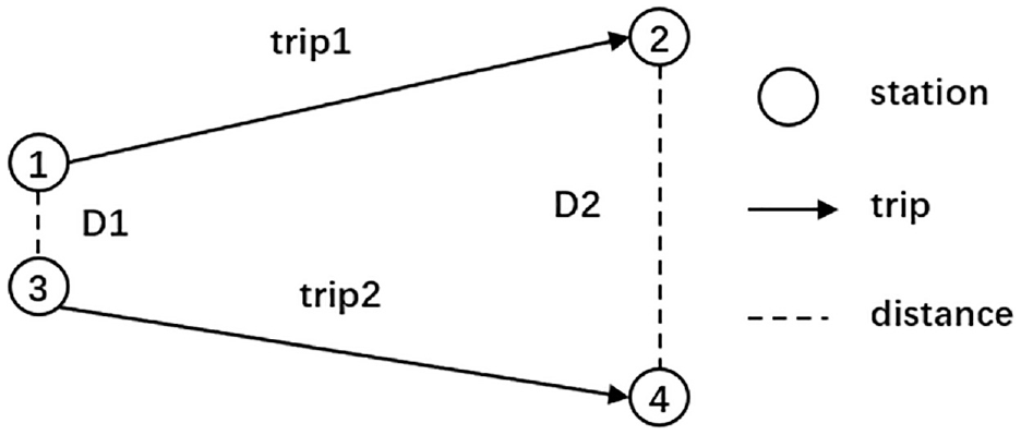
As shown in Figure 3, $D_{1}$ is the Euclidean distance between the boarding stations of the two trips, and $D_{2}$ is the Euclidean distance between the alighting stations of the two trips. $D$ is the distance between two trips defined in this paper. The reason for multiplying by 1,000 is to convert units from kilometers to meters.

Figure 3.

Distance diagram between travel patterns.

To obtain follow-up passenger travel prediction results accurate to the station, the $Eps 2$ is set to 0. The $Eps 1$ and the $MinPts$ is set to 1 hour and 4, respectively, by combining the research of Ma et al. ( 20 ) and the actual data of Chengdu.

Therefore, the algorithm of travel pattern identification is as follows:

Step 1: Randomly extract one unused record from the passenger travel data set, mark it as used and form a cluster;

Step 2: Check the boarding time difference between unused records and the record just extracted. If the different is less than 1 hour, move to step 3, else repeat step 1;

Step 3: Check the spatial distance between unused records and the record just extracted. If it is equal to 0 m, mark the record as used and store it in the cluster generated in the first step, else repeat step 1;

Step 4: For each cluster, if the number of records contained is less than 4, all records in the cluster will be marked as noise; If it is equal to or greater than 4, it will be confirmed as a new cluster category;

Step 5: Continue steps 1 through step 4 until all records in the data set are marked as used.

Step 6: Extract the data of another passenger and repeat steps 1 to 5 until the data of all passengers are marked.

For the trips for which we can obtain a travel pattern, we use the prediction method based on travel pattern, and the method is represented by TP in the following. The prediction method is shown in Equations 12 to 15:

\begin{matrix} P 1' = P (y_{1} | F) \end{matrix}

(12)

\begin{matrix} P 2' = P (y_{i} | M_{i - 1}) \end{matrix}

(13)

\begin{matrix} P 3' = P (M_{1} | F) \end{matrix}

(14)

\begin{matrix} P 4' = P (M_{i} | M_{i - 1}) \end{matrix}

(15)

On the basis of TI, TP uses travel pattern $M$ instead of travel information combination, and the specific prediction method is the same as TI.

Case Study

Result of Travel Pattern Identification

This paper takes the card number 30001746 as an example, and the travel pattern results obtained by the method above are as follows (Table 3).

Table 3.

Example of Identification Results of Passenger Travel Pattern

Consumeday	Cardno	Boarding time	Boarding station	Alighting time	Alighting station	Pattern
2019/5/2	30001746	18:57:38	Jinjiang Hotel station	19:08:48	Tongzilin station	1
2019/5/3	30001746	13:40:28	Tongzilin station	13:58:36	Daye station	2
2019/5/3	30001746	18:33:39	Jinjiang Hotel station	18:41:53	Tongzilin station	1
2019/5/5	30001746	13:49:32	Tongzilin station	14:07:54	Daye station	2
2019/5/5	30001746	18:55:50	Jinjiang Hotel station	19:09:38	Tongzilin station	1
2019/5/9	30001746	13:03:34	Tongzilin station	13:24:58	Daye station	2
2019/5/9	30001746	18:54:18	Jinjiang Hotel station	19:06:33	Tongzilin station	1

Analyzing the proportion of travel patterns for all research objects, the number of journeys with pattern is 532,503,323, which accounts for 32.3% of the total number of trips.

Result of Prediction

This paper randomly selects 10 passengers as a sample to make predictions. Taking the first 3 weeks of the data as the training set to predict the travel information for the fourth week, this paper compares the two methods of TI and TP. The overall prediction results are shown in Table 4. The prediction accuracy in the table is equal to the number of correct predictions in the travel data divided by the total number of travel data. The correct prediction in this paper refers to the correct prediction of the overall travel information, which means that the difference between the predicted time and the actual value is less than 1 h (this is to correspond to the threshold of $Eps 1$ in the travel pattern), and the predicted value of the boarding station and the alighting station is the same as the actual value.

Table 4.

Comparison of Overall Prediction Results

Method of prediction	Accuracy of all travel prediction (100% trips)	Accuracy of travel prediction with travel patterns (37% trips)
TI (%)	24	28
TP (%)	30	41

It can be seen from Table 4 that the overall prediction accuracy of TP is improved by 6% compared with TI. Further analysis of travel prediction accuracy with travel pattern (37% of trips have travel pattern), TP accuracy is 41%, which is 13% higher than TI. This shows that TP has a better predictive effect in travel with travel patterns.

We further analyze the travel with travel patterns, and compare the accuracy rates of the four questions in Table 5. For the two classification problems of whether to travel such as P1 and P3, the prediction accuracy between TI and TP is similar in general. Although there is a 2% drop on P3, this is mainly because of the volatility of the data. For the prediction of travel information, there is a significant improvement between the two methods. The prediction accuracy of P2 has been improved by 11%, and the prediction accuracy of P4 has been improved by 15%. This shows that the method that based on the travel pattern has a certain improvement in the prediction of travel information.

Table 5.

Comparison of Travel Prediction Results With Travel Patterns

Method of prediction	Trips with travel patterns
Method of prediction	P1	P2	P3	P4
TI (%)	87	23	62	29
TP (%)	93	34	60	44

Further analysis the accuracy of travel prediction at different stages with travel patterns, as shown in Figure 4, we find that no matter which method is used, it shows a gradual upward trend except for the first trip each day, and the prediction results of TP are all higher than TI. However, as many trips are mainly concentrated in stages 1 to 3, the overall prediction improvement is not as obvious as shown in Figure 4. Through further analysis, it can be found that the rates of increase of the two lines in Figure 4 are similar, which means applying the clustering method can extract the most likely travel pattern from different combinations of next travel (start time, origin, and destination) to improve the prediction accuracy.

Figure 4.

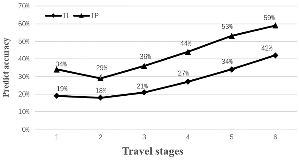
Comparison of prediction accuracy in different travel stages.

In summary, the use of travel patterns can effectively improve the prediction accuracy of passenger travel information. Although the overall improvement is only 6%, the prediction accuracy is increased by 13% for the trips with travel patterns. This shows that it is effective to introduce the concept of travel pattern in the field of bus passenger travel prediction.

Discussion

As shown in Figure 1, the distribution of bus stations in downtown Chengdu is very dense. Considering the arrival of the bus, passengers may choose similar routes to reach a neighboring station for the same destination instead of choosing the same boarding and alighting stations every time. So, as shown in Figure 5, it is reasonable to use active areas to replace stations when the prediction does not need to be accurate for each station ( 21 ).

Figure 5.

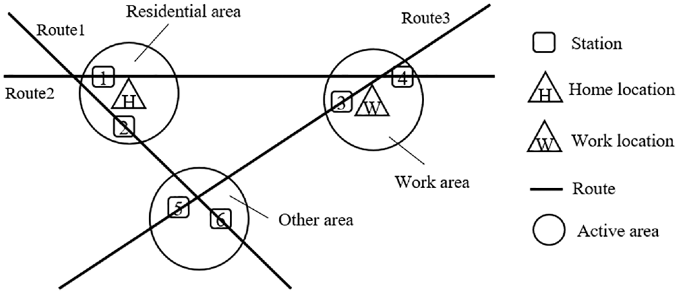
Schematic diagram of station distribution in passenger activity area.

In this paper, we experimentally set the threshold of $D$ for the spatial distance in Equation 11 to 500 m, and the others remain unchanged. The final calculation results are as follows: number of trips with pattern is 6,236,045, which accounts for 37.8% of the total number of trips. And compared with the method that is accurate to the station, the calculation success rate has increased by 5.5%. The reason is that some travel patterns are combined into a travel pattern, which merges some trips with insufficient travel times. As Table 6 shows, the distance between Jinjiang Hotel station and Huaxibai Station is about 400 m, so they are considered the same pattern of travel.

Table 6.

Example of Pattern Fusion

Consumeday	Cardno	Boarding time	Boarding station	Alighting time	Alighting station	Pattern
2019/5/3	30001746	18:33:39	Jinjiang Hotel station	18:41:53	Tongzilin station	1
2019/5/13	30001746	18:25:27	Huaxibai station	18:36:21	Tongzilin station	1

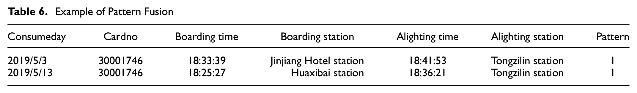
We define the method of predicting using the modified travel pattern based on active areas as TP’. The prediction results of TP and TP’ are compared, as shown in Table 7. The accuracy of all travel prediction has been improved by 5%, and the accuracy of travel prediction with travel patterns has been improved by 9%.

Table 7.

Comparison of Overall Prediction Results

Method of prediction	Accuracy of all travel prediction	Proportion of travel patterns	Accuracy of travel prediction with travel patterns
TP (%)	30	37	41
TP’ (%)	35	42	50

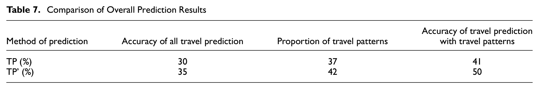
We further analyzed the trips with travel patterns, and the comparison results of the four questions are shown in Table 8. For both P2 and P4, TP’ is increased by 8%. This shows that under the premise of reducing the accuracy of spatial prediction, relaxing the spatial threshold can effectively improve the prediction results.

Table 8.

Comparison of Travel Prediction Results With Travel Patterns

Method of prediction	Trips with travel patterns
Method of prediction	P1	P2	P3	P4
TP (%)	93	34	60	44
TP’ (%)	93	42	60	52

Conclusions

This paper proposes an individual travel prediction algorithm based on travel pattern by using the travel data of bus passengers. When predicting individual travel information, the algorithm first excavates the individual historical travel rules, and integrates the travel information into travel pattern for prediction. First, this paper uses the DBSCAN algorithm to cluster the historical travel of passengers in space and time, so as to obtain the travel patterns of passengers, then uses the travel patterns to dynamically predict the next journey of individuals, and verifies it by using the data of frequent bus passengers in Chengdu, which proves that this method can effectively improve the prediction results. In addition, this paper also discusses the use of active areas instead of stations to identify travel patterns and predict passengers’ travel, and the result shows that the identification of travel patterns based on active areas can improve the prediction further.

The innovation of this paper is mainly to introduce the concept of the travel pattern into the field of individual travel prediction of frequent bus passengers, and in the identification of travel pattern, considering the choice of space thresholds, a station-based prediction method and an activity area-based method are proposed. This effectively improves the prediction effect. In previous studies, the improvement of the prediction effect was mainly focused on the improvement of the algorithm; this paper shifted the focus from the algorithm to the data, and proposed methods to improve the prediction effect from the mining of passenger travel rules.

There are still a couple of shortcomings in this paper: (1) There is no objective basis for the selection of the threshold of travel pattern. Through the Discussion, it can be found that enlarging the threshold can effectively improve the prediction results, but it will also reduce the accuracy of the spatial prediction. (2) Because of time and technical reasons, only a part of the samples is selected for testing in this paper. The universality of the algorithm still needs further verification.

Based on the shortcomings summarized above, we have the following prospects for future research directions: (1) As the thresholds for travel pattern clustering are artificially defined, a scientific method is required to dynamically determine the thresholds according to different data and different research demands. (2) The impact of passenger travel behavior (such as transfers and number of interchanges, etc.) on travel pattern clustering and individual travel prediction needs to be further studied. (3) Algorithm problem: The efficiency of prediction algorithm needs to be improved for larger samples and practical application scenarios. In addition, as the main research content of this paper is the application effect of travel pattern in the field of individual travel prediction, the influence of different algorithms on the prediction results is not studied, which also needs further research in the future.

Footnotes

Author Contributions

The authors confirm contribution to the paper as follows: Study conception and design: Ye, Ma; Data collection: Ye; Analysis and interpretation of results: Ye, Ma; Draft manuscript preparation: Ye, Ma. All authors reviewed the results and approved the final version of the manuscript.

Declaration of Conflicting Interests

The author(s) declared no potential conflicts of interest with respect to the research, authorship, and/or publication of this article.

Funding

The author(s) received no financial support for the research, authorship, and/or publication of this article.

References

Zhao

Koutsopoulos

H. N.

Zhao

Individual Travel Prediction Using Transit Smart Card Data. Transportation Research Part C: Emerging Technologies, Vol. 89, 2018, pp. 19–34.

Song

Blumm

Barabási

A.-L.

Limits of Predictability in Human Mobility. Science, Vol. 327, No. 5968, 2010, pp. 1018–1021.

Bartosz

Sitko

Kazakopoulos

Beinat

Collective Prediction of Individual Mobility Traces for Users With Short Data History. PLoS One, Vol. 12, No. 1, 2017, p. e0170907.

Sapiezynski

Arkadiusz

Gatej

Lehmann

Tracking Human Mobility Using WiFi Signals. PLoS One, Vol. 10, No. 7, 2015, p. e0130824.

Zhao

Musolesi

Hui

, et al. Explaining the Power-law Distribution of Human Travel Through Transportation Modality Decomposition. Scientific Reports, Vol. 5, 2014, p. 9136.

Zhao

Koutsopoulos

H. N.

Individual-Level Trip Detection Using Sparse Call Detail Record Data Based on Supervised Statistical Lear. Presented at 95th Annual Meeting of the Transportation Research Board, Washington, D.C., 2016.

Zhong

Manley

Mller Arisona

Batty

Schmitt

Measuring Variability of Mobility Patterns From Multiday Smart-Card Data. Journal of Computational Science, Vol. 9, 2015, pp. 125–130.

Hasan

Schneider

C. M.

Ukkusuri

S. V.

Gonzlez

M. C.

Spatiotemporal Patterns of Urban Human Mobility. Journal of Statistical Physics, Vol. 151, 2012, pp. 304–318.

Goulet-Langlois

Koutsopoulos

H. N.

Zhao

Measuring Regularity of Individual Travel Patterns. IEEE Transactions on Intelligent Transportation Systems, Vol. 19, 2018, pp. 1583–1592.

10.

Wetter

Bharti

Tatem

A. J.

Bengtsson

Approaching the Limit of Predictability in Human Mobility. Scientific Reports, Vol. 3, 2013, pp. 1–9.

11.

Gambs

Killijian

M.-O.

Del Prado Cortez

M. N.

Next Place Prediction Using Mobility Markov Chains. Proc., First Workshop on Measurement, Privacy, and Mobility MPM’12, Bern, Switzerland, ACM, New York, NY, 2012, pp. 3:1–3:6.

12.

Alvarez-Lozano

García-Macías

J. A.

Chávez

Crowd Location Forecasting at Points of Interest. International Journal of Ad Hoc and Ubiquitous Computing, Vol. 18, No. 4, 2015, pp. 191–204.

13.

Wang

, et al. Segmented Trajectory Clustering-Based Destination Prediction in IoVs. IEEE Access, Vol. 8, 2020, pp. 98999–99009.

14.

Zhong

Tian

Uncovering Quasi-Periodicity of Transit Behavior Based on Smart Card Data. Journal of Transport Geography, Vol. 79, pp. 102466–1024762019.

15.

Medina

S. A. O.

Inferring Weekly Primary Activity Patterns Using Public Transport Smart Card Data and a Household Travel Survey. Travel Behaviour and Society, Vol. 12, 2018, pp. 93–101.

16.

Barry

J. J.

Newhouser

Rahbee

Sayeda

Origin and Destination Estimation in New York City With Automated Fare System Data. Transportation Research Record: Journal of the Transportation Research Board, 2002. 1817: 183–187.

17.

Zhao

Rahbee

Wilson

N. H. M.

Estimating a Rail Passenger Trip Origin–Destination Matrix Using Automatic Data Collection Systems. Computer-Aided Civil and Infrastructure Engineering, Vol. 22, No. 5, 2007, pp. 376–387.

18.

Wang

Attanucci

Wilson

N. H. M.

Bus Passenger Origin-Destination Estimation and Related Analyses Using Automated Data Collection Systems. Journal of Public Transportation, Vol. 14, No. 4, 2011, pp. 131–150.

19.

Nassir

Hickman

Z. L.

Activity Detection and Transfer Identification for Public Transit Fare Card Data. Transportation, Vol. 42, No. 4, 2015, pp. 683–705.

20.

Y. J.

Wang

Chen

Liu

Mining Smart Card Data for Transit Riders’ Travel Patterns. Transportation Research Part C: Emerging Technologies, Vol. 36, 2013, pp. 1–12.

21.

Wei

Reconstruction and Analysis of Bus Travel Behavior Based on Activity Recognition. Journal of Transportation Systems Engineering and Information Technology, Vol. 20, No. 4, 2020, pp. 143–149.