Emissions and Air Quality Implications of Enabling On-Road Vehicles as Flexible Load Through Widescale Zero Emission Vehicle Deployment in California

Abstract

This study assesses the impacts of on-road light- to heavy-duty zero emission vehicle (ZEV) adoption and charging protocols on greenhouse gas emissions for the years 2030 and 2045 in California, and on air quality for the year 2045. Two scenarios are addressed: (1) a “business-as-usual” (BAU) scenario with modest ZEV adoption, and (2) a “carbon neutral” scenario that achieves carbon neutrality by 2045 with proactive ZEV adoption. Electricity load for fueling ZEVs is projected, including electricity fuel for battery electric vehicles and electrolytic hydrogen for fuel cell electric vehicles. This electric load was input into an electric grid dispatch model and electric grid and air quality analyses were conducted. The results revealed that although medium- and heavy-duty vehicles (MHDVs) are projected to have lower total electric load associated with fueling, they will require roughly double the electricity for hydrogen production of light-duty vehicles. For the electric grid scenarios examined, ZEV loads increased peak electricity demand by 3% to 6% in 2030 and 22% to 31% in 2045. MHDV time-of-use and smart charging strategies were equally able to shift charging demand to off-peak times. Higher ZEV loads under the carbon neutral scenario increased natural gas use up to 6% in 2030 and energy storage requirements up to 45% in 2045 compared with the BAU scenario. The analyses also found that achieving carbon neutrality through ZEV adoption had the cobenefit of significantly reducing ground-level ozone and PM_2.5 concentrations in key regions of California, providing health savings of approximately $28 billion annually in 2045.

Keywords

transportation and sustainability electric and hybrid-electric vehicles hydrogen/fuel cells electricity grid regional and state planning

The present study conducted a novel assessment of the air quality and health benefits of an on-road vehicle scenario with coordinated electric vehicle charging and electrolytic hydrogen production toward the goal of carbon neutrality. The commitment to reduce greenhouse gas (GHG) emissions in response to climate change and criteria air pollutant (CAP) emissions in response to degraded air quality has initiated the widespread deployment of renewable energy technologies and zero emission vehicles (ZEVs) in the form of battery electric vehicles (BEVs) and fuel cell electric vehicles (FCEVs). In California, the electric grid is becoming increasingly renewable to meet legislation such as California Assembly Bill 32 ( 1 ), Senate Bill 32 ( 2 ), and ultimately Senate Bill 100, which requires all retail electricity sold in the state to be from zero carbon sources by 2045 with the preceding two bills being touchstones along the way ( 3 ). In the transportation sector, ZEV deployment has initially focused on light-duty vehicles (LDVs) and much of the research on both the charging infrastructure and vehicle requirements has focused on the needs of the light-duty sector. However, low- and zero emission powertrain technologies for medium- and heavy-duty vehicles (MHDVs) are starting to enter the marketplace as regulations such as the California Air Resources Board’s (CARB’s) Advanced Clean Trucks regulation come into effect. To meet the aggressive goal of carbon neutrality by 2045, emissions from all on-road vehicles need to be addressed.

MHDVs are a major source of both GHG and CAP emissions including oxides of nitrogen (NO_x) and particulate matter (PM) ( 4 , 5 ). In California, LDVs and MHDVs collectively represent one of the foremost sources of CAP, including 45% of statewide NO_x ( 6 ), which contributes to degraded air quality and subsequent health damage in exposed populations ( 7 ). MHDVs are of particular concern because of the current reliance on diesel fuel, which generates diesel PM and other toxic air contaminants that have acute, local health effects when combusted, in addition to contributing emissions of NO_x, which add to regional burdens of PM_2.5 and ozone ( 8 , 9 ). Therefore, transition to ZEVs operating on low carbon fuels will be necessary to achieve California’s environmental quality goals; ZEVs have been shown to provide significant benefits to air quality and health when deployed at scale ( 10 ).

For the electric grid, while the growth in solar and wind capacity reduces overall emissions, it introduces new challenges, such as renewable intermittency, which requires balancing resources (e.g., thermal plants, energy storage) to be more flexible, as characterized by faster response times and ramp rates, as well as fewer constraints on minimum uptime and downtime ( 11 ). The deployment of ZEVs introduces new loads onto the grid either through BEV charging or through electrolytic fuel production. If these new loads are not coordinated with renewable availability, they could increase the peak demand and ramping requirements of balancing resources, as well as overall reliance on fossil fuel-powered generation. Therefore, understanding the potential for coordinated electric vehicle charging and electrolytic hydrogen production is crucial for ensuring overall emissions reduction goals are met. Quantifying these metrics is the novel research question of the present work.

Literature Review

Previous literature has shown that to achieve the emissions reduction potential of a high renewable portfolio, variable renewable generation (solar and wind) needs to be partnered with low- to zero emission resources that can respond dynamically to maintain grid performance ( 12 – 19 ). At the same time, most sectors are looking to electrify their energy demands, providing an opportunity to utilize these new loads as flexible grid resources to smooth the intermittency of variable renewable generation (Schuller et al. [ 20 ]).

Transitioning to ZEVs can significantly reduce emissions from the transportation sector, but it can also result in increased energy demand on the electric grid. This demand can come either directly through vehicle charging or indirectly through the production of electrolytic fuels ( 21 ). The added demand can increase grid-related emissions if renewable availability and other grid dynamics are not considered ( 22 , 23 ). Coordinating the charging of connected vehicles with renewable electricity availability can offset the required capacity of other grid resources, such as natural gas power plants and energy storage, reducing system costs and ensuring emissions reductions. Factors affecting vehicle flexibility to balance the grid include vehicle state of charge (SOC), electric vehicle supply equipment (EVSE) location and charging rate, dwell time, charging intelligence, and travel constraints ( 24 , 25 ).

LDVs tend to be operated by individuals for personal use, traveling mostly between home and work but also numerous other locations that can vary by day and time of year, which in turn affect daily fuel consumption patterns and a BEV’s access to EVSE ( 26 , 27 ). MHDVs tend to operate in fleets, with many following a regular driving schedule and duty cycle, making them amenable to grid coordination efforts ( 28 ). Therefore, MHDVs are potentially a streamlined avenue for grid and vehicle coordination through delayed, time-of-use, or smart charging compared with other vehicles. Most studies examining the dynamics of vehicle–grid integration have focused on plug-in LDVs ( 12 , 29 –32). Previous studies examining plug-in MHDV charging dynamics in detail tend to focus on the deployment of a limited number of vehicles and/or do not explore the net impact on the electric grid ( 22 , 33 , 34 ). A limited number of studies have examined the feasibility of ZEVs for the medium- and heavy-duty sectors ( 35 – 37 ). These studies provide insights into the limits of ZEV deployment as well as the technical parameters required to achieve a desired level of ZEV adoption. By accepting the technical constraints for medium- and heavy-duty ZEVs, the future grid impacts of their deployment can be assessed and their potential for reducing GHG and CAP emissions quantified.

To project the potential benefit of deploying on-road ZEVs, first, a projection for the deployment of ZEVs and their fuel demand must be made. This projection must differentiate between BEVs and FCEVs, as well as how the hydrogen for the FCEVs will be made. Electrolytic hydrogen will require significant electricity input, whereas bio-derived hydrogen is relatively electric grid–independent. Projections for ZEV deployment and the resulting fuel demand have included the use of optimization algorithms, such as those by Angeles et al. ( 38 ), Ribau et al. ( 39 ), and Samsatli and Samsatli ( 40 ). These works include various fuels and powertrain configurations, but do not include the full breadth of on-road transportation from LDVs to heavy-duty vehicles. An alternative approach is through vehicle stock modeling and enforcing a transition plan, which is needed to meet desired goals such as carbon neutrality. This approach is taken by Brown et al. ( 41 ) and includes both LDVs and MHDVs. This latter approach was used in the present work as a comprehensive view of the on-road vehicle categories required.

Previous work has assessed the impacts of on-road vehicles on future ozone and PM_2.5 concentrations relative to other transportation subsectors as a whole ( 42 ). Researchers have additionally examined the use of emissions control and carbon pricing to mitigate freight-related air quality and health damage for the United States ( 43 ). Several studies have reported air quality and health benefits from the use of ZEVs and low NO_x compressed natural gas vehicles within portfolios of climate mitigation strategies, but the studies did not isolate those strictly from on-road transportation and did not target carbon neutrality ( 44 – 47 ). The air quality impacts of deploying high levels of hydrogen fuel cell electric LDVs and MHDVs have been assessed, but only included episodic air quality simulations (i.e., 2 weeks) and did not include health effects ( 48 ). Therefore, to date, no study has conducted a comprehensive assessment of the air quality and health benefits of an on-road vehicle scenario with the goal of reaching carbon neutrality.

Methods

The process in the present work was as follows. First, electric grid demand and ZEV fuel demand projections for LDVs and MHDVs were gathered from the literature. The downstream analyses used the two following scenarios, adopted by Brown et al. ( 41 ): (1) a “business-as-usual” (BAU) scenario with limited ZEV deployment, and (2) a “carbon neutral” (CN) scenario that aims to meet carbon neutrality by 2045, as asserted by California Executive Order B-55-18.

The hydrogen fuel demand projections were processed according to a Monte Carlo simulation (MCS) of the hydrogen market to determine what fraction of hydrogen will come from electrolyzers and therefore use electricity as a primary feedstock. Lane et al. developed this methodology using MCS surrounding a technoeconomic analysis ( 49 ), and the present analysis applied this methodology to determine the projected electricity load from hydrogen production for LDVs and MHDVs.

The resulting electricity demands for fueling BEVs and producing electrolytic hydrogen for fueling FCEVs were the inputs to simulations of the California electric grid using an electric grid dispatch model, Holistic Grid Resource Integration and Deployment (HiGRID). The results from HiGRID included the temporally resolved use of electric grid resources, the charging of BEVs, the production of electrolytic hydrogen fuel, and the resulting emissions of both average and marginal electricity production.

Projecting Electricity Load From Zero Emission Vehicle Deployment

This study calculated the electricity load for vehicle fuel, either directly as electricity or indirectly through electrolytic hydrogen, using annual demand from the BAU and Low Carbon (LC1) scenarios of Brown et al. ( 41 ) as a starting point for the BAU and CN scenarios of the present study, respectively. The primary distinction between the BAU and CN scenarios was the amount of ZEV adoption, which affects the quantity of electricity and hydrogen projected for on-road transportation fuel. The hydrogen demand was further categorized by feedstock type. The present work focused on the portion of hydrogen produced from electricity feedstock through electrolyzers, which served as an input into the electric grid modeling that followed.

To determine the quantity of electrolytic hydrogen, this study used a stochastic market competition model developed by Lane et al. ( 49 ). That work conducted a technoeconomic analysis of the two primary competing renewable hydrogen production methods: electrolytic and thermochemical conversion of biomass. Given an initial market condition, a technology efficiency projection, and ranges for possible hydrogen market size, this study conducted a series of MCSs in which the two production technologies competed for the lowest cost production of hydrogen. The result is a market composition for renewable hydrogen, and the present study applies the fraction of hydrogen that is expected to be electrolytic. From this quantity of hydrogen, electrolyzer efficiency was used to determine the associated electricity load, which was then put into the HiGRID electric grid model.

Electric Grid Modeling

This analysis applied the HiGRID tool to simulate the impact of vehicle integration with the future California electric grid. HiGRID is an hourly resolved electric grid resource dispatch model that determines the response of different electric grid resources to satisfy the statewide electric load demand and grid service requirements. In summary, HiGRID operates in three steps. First, HiGRID takes as inputs the capacities of renewable electricity resources and calculates their hourly resolved generation profile for the year. The aggregate renewable generation profile is subtracted from the aggregate nondispatchable load profiles to determine the initial net load profile. Second, the dispatch of flexible loads, such as grid-communicative BEV charging, is calculated in response to the initial net load, then added to it to compose a final net load. Third, the dispatch of controllable electricity generation resources (i.e., hydropower, etc.) is calculated to satisfy the remaining unmet load and ancillary service requirements, and the extent to which the variable renewable electricity may need to be curtailed to ensure that the load is balanced is also calculated. HiGRID has previously been leveraged to assess different aspects of the integration of plug-in electric vehicles with the grid, such as the importance of flexible charging for LDV emissions reduction ( 50 ), the effect of flexible charging and vehicle-to-grid operation on grid planning requirements ( 23 ), and the value of flexible charging and vehicle-to-grid operation for passenger vehicles ( 51 ).

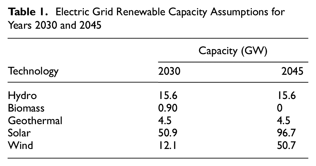
The BAU load profiles for 2030 and 2045 combine (a) the Energy Environmental Economics (E3) PATHWAYS baseline projections of electric load profiles (excluding on-road transportation) ( 52 ); (b) the on-road BEV load profiles, calculated in the BEV charging model described in the next section; and (c) the electrolytic hydrogen production profile, which is calculated in HiGRID. The E3 PATHWAYS study was a previous economywide planning study conducted by E3 to determine what is required from a technology deployment standpoint to meet California’s previous goal of 80% reduction in economywide GHG emissions by 2050. The baseline renewable capacity from PATHWAYS was also assumed (see Table 1). The 2030 generation portfolio meets the 60% renewable portfolio standard target and the 2045 portfolio meets the carbon neutrality target through a combination of renewable generation, hydropower, and energy storage. The increase in ZEV electricity demand in the CN scenarios can have positive or negative impacts on grid emissions depending on vehicle–grid interactions.

Table 1.

Electric Grid Renewable Capacity Assumptions for Years 2030 and 2045

Technology	Capacity (GW)
Technology	2030	2045
Hydro	15.6	15.6
Biomass	0.90	0
Geothermal	4.5	4.5
Solar	50.9	96.7
Wind	12.1	50.7

Battery Electric Vehicle Charging Model

The BEV charging model in this study combined the LDV charging model from Zhang ( 53 ) and the MHDV charging model from Forrest et al. ( 37 ). The charging models utilized trip-based travel datasets calibrated to match California in-state, category-specific travel demands and dwell constraints to determine charging electricity demand under different EVSE infrastructure assumptions. The two main dwell constraints were the length of time a vehicle is parked between trips (“dwell periods”) and the type of dwell locations (e.g., home, work). EVSE infrastructure assumptions included the types of dwell locations that had EVSE and the charging rate that was available at each location type. The MHDV immediate charging model was previously applied in Forrest et al. ( 37 ), and this analysis introduced two MHDV charging scheduling approaches: time-of-use (TOU) utility rate structure and smart charging. These scheduling strategies were adapted from the LDV charging model developed by Zhang ( 53 ).

The cost function is as follows ( 53 ):

\min (\begin{matrix} \sum_{j = 1}^{q} f_{j} \times x_{j} \end{matrix})

(1)

where

f = electricity cost per kWh,

x = increase in SOC (kWh),

j = dwell segment, and

q = total number of dwell segments.

The equality constraint is

\begin{matrix} \sum_{j = 1}^{q} \end{matrix} x_{j} + \begin{matrix} \sum_{i = 1}^{m} \end{matrix} y_{i} = 0

(2)

where

i = trip number,

y = discharged energy (kWh), and

m = total number of trips.

The inequality constraints are

y_{1} > - c

(3)

y_{1} + \begin{matrix} \sum_{j = 1}^{q} \end{matrix} x_{1 j} + y_{2} + \dots + \begin{matrix} \sum_{j = 1}^{m - 1} \end{matrix} x_{(m - 1) j} + y_{m} > - c

(4)

where c = battery energy capacity.

Bounds on the variables are

0 \leq x_{ij} \leq p_{j} \times Δ t_{ij} \times η

(5)

where

p = rated power capacity (kW) of EVSE,

Δt = dwell time (h), and

η = charging efficiency.

The cost function (Equation 1) minimizes the cost of charging each BEV, subject to the equality (Equation 2) and inequality constraints (Equations 3 and 4). The equality constraint requires that the electricity delivered to the vehicle is equal to the electricity discharged during trips. The inequality constraints ensure that the amount of electricity discharged during trips never exceeds the capacity of the battery. Equation 3 requires that for the first trip, the discharged energy does not exceed the battery capacity. Equation 4 applies a similar constraint for each following trip (y_i) and charging (x_(i-1)j) pair, that is, the battery SOC at the end of a trip never falls below zero and the battery SOC after a charging event never exceeds the maximum battery capacity. Lastly, the bounds (Equation 5) ensure that the electricity delivered to the vehicle is less than or equal to the maximum transferrable energy through the EVSE. The maximum transferrable energy is limited by the rated power of the EVSE (p), the dwell time following each trip (Δt), and the charging efficiency (i.e., the ratio of energy available to discharge from the battery versus the energy supplied).

For TOU charging, the vehicle charging was planned around a basic cost function with three rates set by time of day. For this analysis, the Pacific Gas and Electric (PGE) business EV TOU rate was applied ( 54 ). The TOU rate applies prices for three distinct periods: peak $ 0.35/kWh (4 to 9 p.m.), off-peak $ 0.14/kWh (midnight to 9 a.m., 2 to 4 p.m., and 9 p.m. to midnight), and super off-peak $ 0.11/kWh (9 a.m. to 2 p.m.). In the real-world application of MHDV charging, electric utilities, including PGE, are planning to combine TOU rates with a flat monthly subscription rate based on peak demand. The tradeoff between limiting peak demand and charging during off-peak and super off-peak times is not quantified in this analysis but is the topic of future work. The limitation of a TOU schedule is that it is structured based on the average grid conditions and does not consider the day-to-day variation in demand and renewable availability.

For smart charging, vehicle charging is scheduled using a cost optimization that applies the hourly net load (load minus renewables) as a proxy for “electricity price.” In general, the lowest cost periods correspond to periods of low or negative net load. (A negative net load indicates that there is excess renewable generation that would be curtailed otherwise.) The smart charging algorithm uses a centralized control approach that updates the cost signal after each connecting vehicle plans its charging schedule, to account for the added load. The model outputs a vehicle electric load profile that is applied within HiGRID to determine the impact of vehicle charging on the electric grid.

The years 2030 and 2045 were the focus of the projected vehicle electricity demands for the BAU and CN scenarios. This analysis assumed that battery electric LDVs have a 200-mi range and charge at home and work using Level 2 charging. Furthermore, it assumed that battery electric MHDVs have a 200-mi range and EVSE are 100 kW located at fleet depot locations (“home base”). For more information on how range and charging rate affect immediate charging profiles, see Zhang et al. ( 32 ) and Forrest et al. ( 37 ).

Air Quality Modeling

Transitions to zero emission vehicles in the CN scenario will reduce CAP emissions relative to the BAU scenario, which will improve regional air quality and subsequently provide health benefits within populations exposed to lower levels of pollution. To quantify and value these benefits in 2045, spatially and temporally resolved characterizations of CAPs were developed for both the CN and BAU scenarios, accounting for differences in vehicle emissions and all major end-use sectors in California. The emissions from on-road vehicles were estimated from a CARB emission inventory, generally informed using EMission FACtor 2021 v1.0.2 ( 55 ). Next, the Community Multiscale Air Quality Modeling System ( 56 ), a photochemical air quality model that accounts for atmospheric chemistry and transport, translated emissions changes into impacts on atmospheric pollution levels, including ground-level ozone and PM_2.5. Changes in pollutant concentrations led to conducting a health impact assessment using the Environmental Benefits Mapping and Analysis Program – Community Edition ( 57 ), which quantifies and values the reductions in mortality and morbidity endpoints that benefit exposed populations. A detailed description of the methodology can be found in Brown et al. ( 41 ).

Results

Figures 1 to 4 depict the projected electricity load associated with the BAU and CN scenarios for both LDVs and MHDVs separately. The figures also differentiate between electricity as a fuel and electricity as a feedstock for producing hydrogen through electrolyzers. Note the difference in y-axis scales. The BAU scenario had less electricity load than the CN scenario owing to the far more limited adoption of ZEVs. Also, the LDVs used more fuel than the MHDVs primarily because of the difference in vehicle miles traveled (VMT) between the vehicles. The substantial use of hydrogen presented is in agreement with work done for the California Environmental Protection Agency ( 41 ) and CARB ( 58 ).

Figure 1.

Business as usual (BAU) scenario electric load for light-duty vehicles (LDV) fuel.

Figure 2.

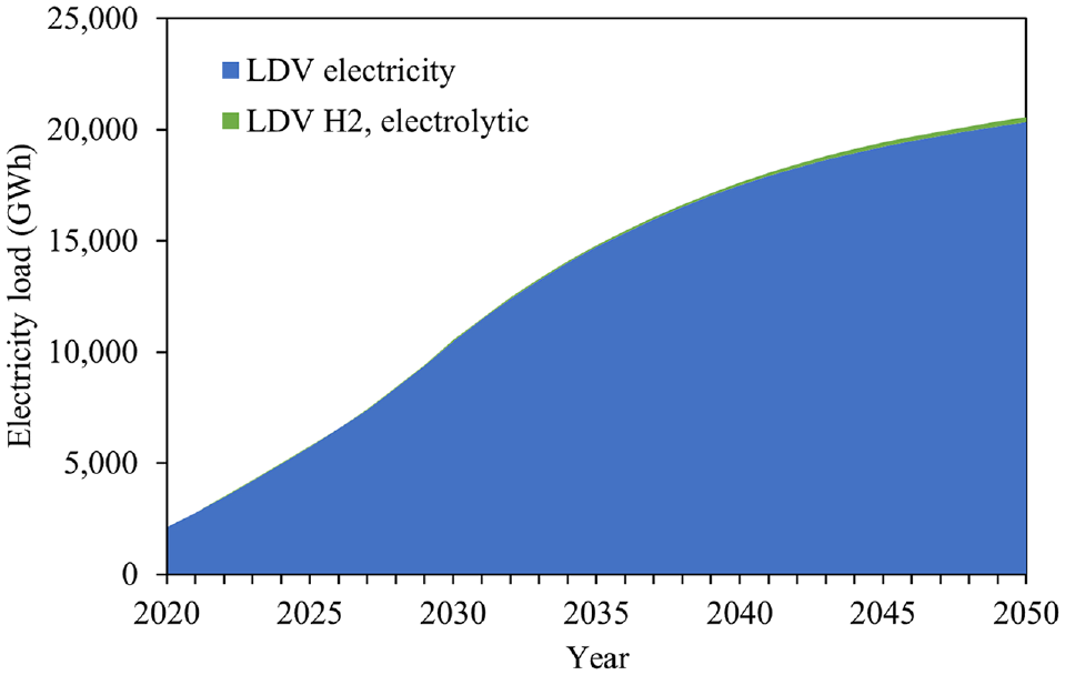
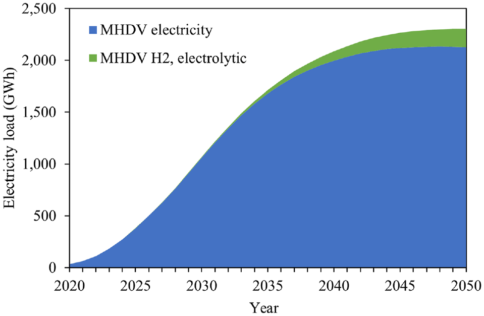
Business as usual (BAU) scenario electric load for medium- and heavy-duty vehicle (MHDV) fuel.

Figure 3.

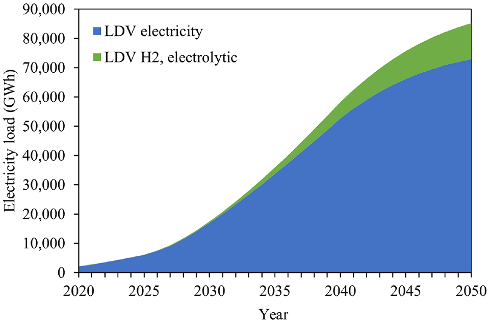
Carbon neutral (CN) scenario electric load for light-duty vehicles (LDV) fuel.

Figure 4.

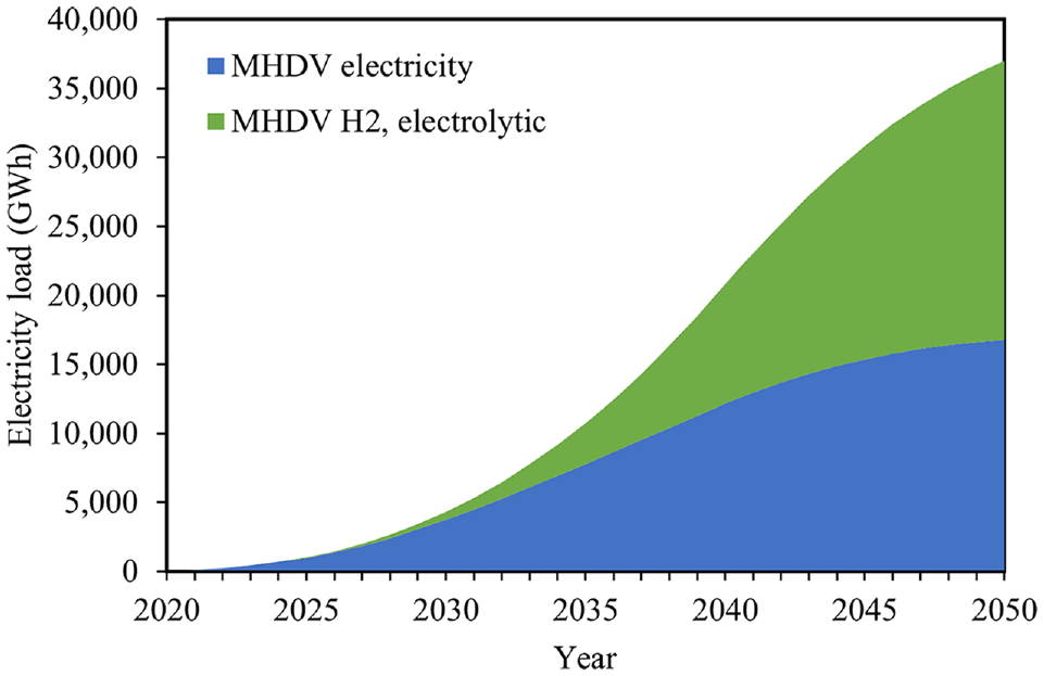
Carbon neutral (CN) scenario electric load for medium- and heavy-duty vehicle (MHDV) fuel.

Figure 5 presents the load demand profiles for an example week for the 2030 and 2045 CN immediate charging scenarios. In 2030, loads that exceed renewable availability must be met through either natural gas load followers or peaker plants. Load followers are combined cycle power plants with moderate ramp rates. Peaker plants are simple-cycle plants with faster ramp rates but are more expensive and more polluting per unit of electricity generated compared with load followers. In 2045, energy storage meets this demand by charging during periods of excess renewables and discharging during periods low, insufficient renewable generation.

Figure 5.

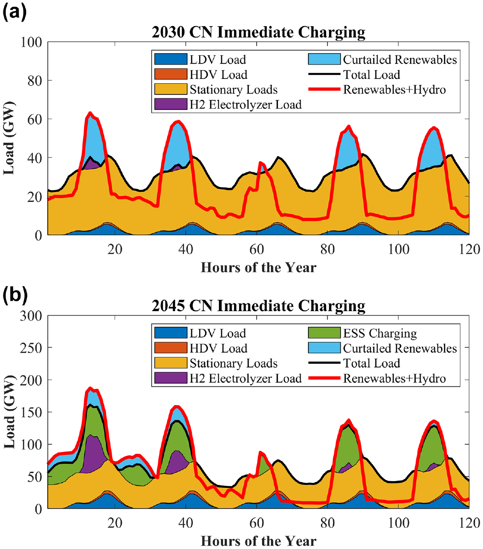
Timeseries of electricity loads in the carbon neutral immediate charging scenarios in (a) 2030 and (b) 2045.

Under the scenario assumptions for 2030 and 2045, immediate charging of LDVs and MHDVs resulted in a charging peak between 6 and 8 p.m.—the same period that stationary loads peak, thus increasing the total peak net load that must be met from balancing resources (in this case, natural gas power plants). Comparing the 2030 BAU with the 2030 CN immediate charging scenario, peak net load increased from 40.3 to 42.6 GW. The CN TOU and smart charging scenarios were equally able to shift MHDV load to off-peak times, resulting in a peak net load of 41.6 GW. The 1.3 GW increase from the BAU in these scenarios was a result of the increased LDV load in the CN scenarios. Hydrogen production is less constrained than vehicle charging, as it is not limited by vehicle dwell periods. Electrolyzer load demand occurred during periods when renewable generation would otherwise be curtailed.

For the CN scenarios, electricity demand for battery electric LDVs and MHDVs between 2030 and 2045 increased by approximately 290% and electricity demand for electrolytic hydrogen increased by nearly 590%. Peak net load for the 2045 CN immediate charging scenario was 72 GW, up 31% from the 2045 BAU. Implementing TOU and smart charging reduced the peak net load relative to the CN immediate charging scenario, both having a peak demand of 66 GW.

Figure 6 presents the 2030 MHDV load demand for each charging strategy. Under the TOU rate strategy, vehicles began charging when the price dropped at 9 p.m., whereas, depending on the net load conditions, the vehicles under the smart charging strategy waited until later. The charging behavior during off-peak times diverged as well. In the example day shown, MHDVs deployed with smart charging scheduled charging to align with the minimum net load and ramped down as the net load increased. TOU was less accurate in timing charging. The net result was higher peaker plant generation for the TOU case, as shown in Figure 7.

Figure 6.

Year 2030 medium- and heavy-duty battery electric vehicle charging demand by charging strategy.

Figure 7.

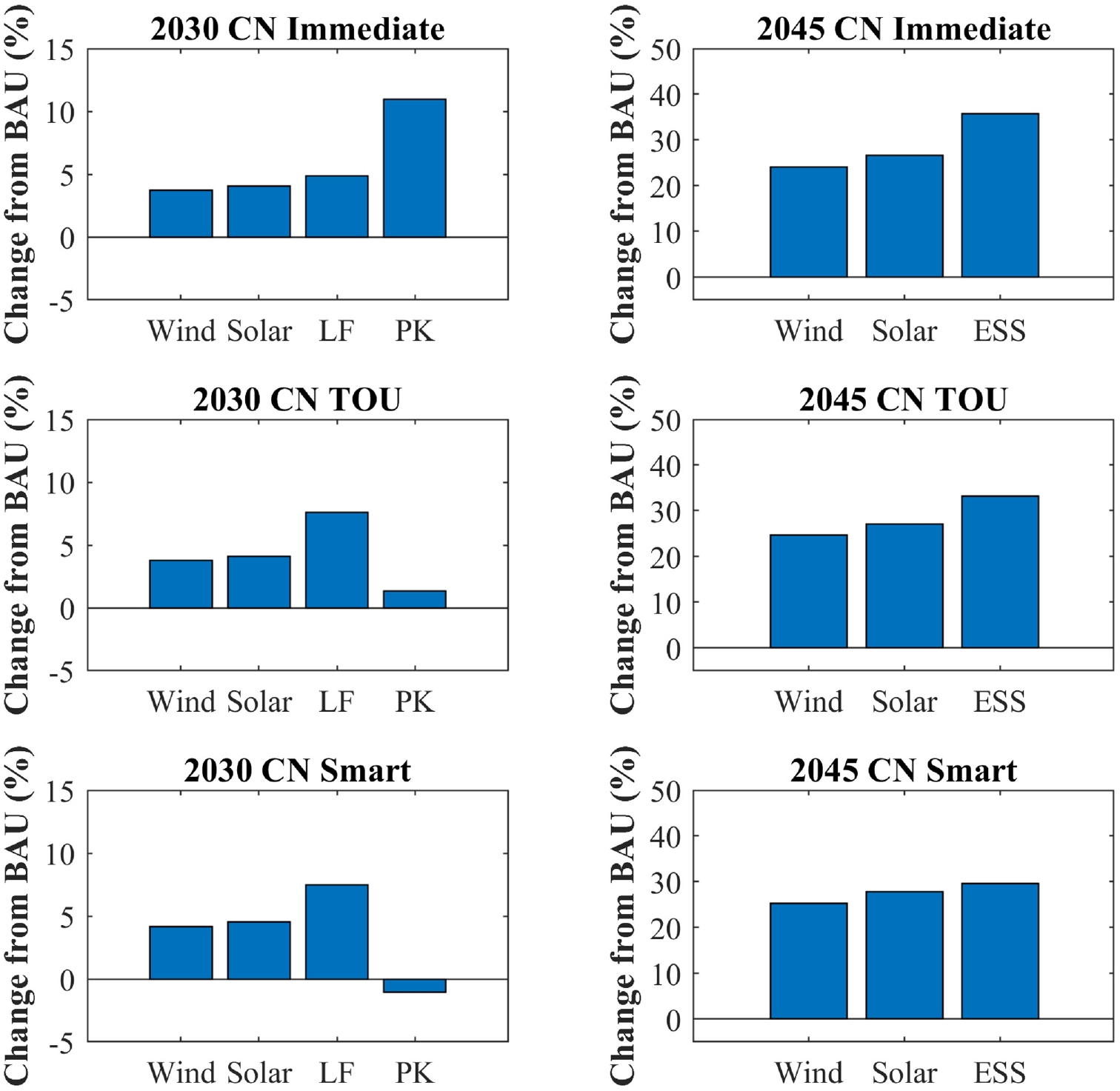
Change is electricity delivered by source for 2030 and 2045 carbon neutral (CN) scenarios, natural gas load follower (LF) plants, natural gas peaker plants (PK), and energy storage systems (ESS).

Figure 7 presents the change in energy delivered by resource. Only resources with a changing contribution of generation are shown. For example, geothermal and hydropower generation remained constant across the scenarios, so they are omitted. In 2045, energy storage was dispatched to balance the net load. The energy storage charges using renewable generation and discharges to meet load. The greater transportation loads in the CN scenarios compared with the BAU resulted in the increased utilization of renewable generation (solar and wind). It also increased the reliance on natural gas power plants, as the battery electric LDV and MHDV loads did not align solely with renewable generation availability. In 2030, switching from immediate charging to TOU reduced natural gas peaker generation by 9%, and switching to smart charging reduced it by 11%. Total generation from natural gas increased by 6% in the CN scenarios compared with the BAU, with total natural gas generation remaining relatively constant (<1% change) between the different charging scenarios. As renewable generation and natural gas use both increased, the calculated renewable penetration remained at 60% ± 0.4%.

In 2045, the CN scenarios resulted in an increase in wind and solar utilization, but also an increase in the energy storage requirements to achieve a CN grid. Switching from MHDV immediate charging to a TOU rate reduced the load that needed to be met by energy storage by 2%, and switching from MHDV immediate charging to smart charging reduced it by 5%.

Figure 8 shows the decarbonization of on-road vehicles in the CN scenario results in improvements in annual PM_2.5 which reach −0.9 μg/m³ in 2045, which is significant considered in the context of the primary annual average PM_2.5 National Ambient Air Quality Standard of 12 μg/m³. Additionally, annual improvements in maximum daily 8-hour average ozone reach −1.5 ppb, including reductions up to −2.8 ppb throughout the ozone season. For both pollutants, the largest impacts occur in Southern California, which aligns with the dense urban population it contains and the current challenges with degraded air quality prominent in the region ( 59 ). Similarly, notable improvements occur in the Central Valley, which frequently experiences unhealthy air quality ( 60 ). The reductions for both pollutants are substantial, and desirable in the locations they occur because of potential health benefits and the support of attainment of Federal health-based regulatory standards ( 61 ). Additionally, the areas that experience the greatest improvements are correlated with the presence of socially and environmentally disadvantaged communities, including in and around the Ports of L.A. and Long Beach, portions of San Bernardino and Riverside Counties, and the Central Valley ( 62 ).

Figure 8.

Difference (in μg/m³) predicted for the carbon neutral (CN) scenario in 2045 for annual average PM_2.5.

Air quality improvements resulted in health savings that exceeded $28 billion (2020 USD) annually in 2045. The majority of avoided mortality incidence was associated with reduced exposure to PM_2.5, estimated to be 3,123 incidences. This contributed approximately $27 billion in benefits. Additionally, PM_2.5 improvements provided reductions in hospitalizations for various deleterious health effects, including cardiovascular and respiratory illness. Improved ozone concentrations were responsible for an additional 111 avoided incidences of mortality, which contributed approximately $1 billion in benefits. Health savings from avoided ozone morbidity events provided only a minor portion of the total health benefits but were notable for significant reductions in hospital admissions for asthmatic episodes. Furthermore, reducing ozone concentrations avoided loss of schooling and restricted activity days for children. Additional details can be found in Brown et al. ( 41 ).

Summary and Conclusions

The present work analyzed the impact of ZEV adoption in both the LDV and MHDV sectors. Projections for two scenarios of the electric load from LDVs and MHDVs incorporated electricity fuel for BEVs and electrolytic hydrogen fuel for FCEVs. These loads were inputs for HiGRID, an electric grid dispatch model. Three charging protocols (immediate, TOU, and smart) were modeled for the CN scenario. The major conclusions from the study follow:

FCEV MHDVs are expected to require roughly 60% more electricity for hydrogen production than FCEV LDVs. Fueling ZEV LDVs is generally expected to require double the electricity of fueling ZEV MHDVs primarily because of higher VMT. However, the powertrain characteristics and duty cycle requirements of FCEV MHDVs are expected to increase the relative adoption of FCEVs for these applications compared with FCEV LDVs. Therefore, a greater amount of electric load is projected for fueling FCEV MHDVs than FCEV LDVs.

BEV MHDVs are expected to require roughly one-quarter of the electricity fuel of BEV LDVs. Fueling ZEV LDVs is generally expected to require double the electricity of fueling ZEV MHDVs primarily because of higher VMT. Further, powertrain characteristics and duty cycle requirements of BEV MHDVs are expected to decrease the relative adoption of BEVs for these applications compared with BEV LDVs. Therefore, a far greater amount of electric load is projected for fueling BEV LDVs than BEV MHDVs.

Increased GHG emissions from the electric grid for the 2030 charging scenarios are more than offset by reductions in GHG emissions from the transportation sector. Although grid emissions increased by up to 6% for the 2030 CN scenarios, the net impact is an overall reduction in the systemwide GHG emissions associated with the reduction of emissions from the transportation sector.

As more sectors are electrified, it will be important to maximize the flexibility of these new loads to maintain grid performance. In this analysis, integrating immediate charging of battery electric LDVs and MHDVs resulted in charging during periods of insufficient renewable generation and increased peak net load. This in turn increased natural gas use in 2030 and the energy storage required to achieve the goal of carbon neutrality in 2045. By increasing vehicle load flexibility, grid performance improved. For example, in 2030, peak net load and peaker generation decreased compared with the immediate charging scenario, and in 2045 there were minor reductions in the load that needed to be balanced by energy storage technologies (2% to 5%).

ZEV on-road vehicles could provide significant socioeconomic benefits through improvements in air quality. The air quality and health benefits estimated here clearly demonstrated the important cobenefits that decarbonizing on-road transportation could achieve. The potential health savings are sizable ($28 billion) and should be considered alongside the possible increased cost of replacing conventional petroleum vehicles. This is particularly true for ZEVs, which attained the largest reductions in emissions. Further, the health savings shown here could occur in populations that are often most negatively affected by air quality and are more vulnerable to the associated health damage ( 63 ).

Footnotes

Acknowledgements

The authors acknowledge the California Air Resources Board, United States, the California Environmental Protection Agency, and the University of California Office of the President for supporting this research.

Author Contributions

The authors confirm contribution to the paper as follows: study conception and design: B. Lane, K. Forrest, S. Samuelsen; data collection: B. Lane, K. Forrest, M. Mac Kinnon; analysis and interpretation of results: K. Forrest, B. Lane, M. Mac Kinnon, S. Samuelsen; draft manuscript preparation: K. Forrest, B. Lane, M. Mac Kinnon, B. Tarroja. All authors reviewed the results and approved the final version of the manuscript.

Declaration of Conflicting Interests

The authors declared no potential conflicts of interest with respect to the research, authorship, and/or publication of this article.

Funding

The authors disclosed receipt of the following financial support for the research, authorship, and/or publication of this article: This research was funded by the Advanced Power and Energy Program, the California Air Resources Board, United States (under contract no. 16RD011), and the California Environmental Protection Agency and the University of California Office of the President (under contract no. UC-ITS-2020-65).

ORCID iDs

Kate Forrest

Blake Lane

Michael Mac Kinnon

Scott Samuelsen

Data Accessibility Statement

Vehicle emissions data inputs are available from https://arb.ca.gov/emfac/. Energy Environmental Economics (E3) PATHWAYS projection data used in this study are available from . Additional data from the updated PATHWAYS project must be requested from E3. Model result data for the study are available on request.

References

AB 32. California Global Warming Solutions Act of 2006. California State Assembly. 2006. https://leginfo.legislature.ca.gov/faces/billNavClient.xhtml?bill_id=200520060AB32

SB 32. California Global Warming Solutions Act of 2006: Emissions Limit. California State Senate. 2016. https://leginfo.legislature.ca.gov/faces/billNavClient.xhtml?bill_id=201520160SB32

SB-100. California Renewables Portfolio Standard Program: Emissions of Greenhouse Gases. 2018. https://leginfo.legislature.ca.gov/faces/billNavClient.xhtml?bill_id=201720180SB100

California Air Resources Board. California Sustainable Freight Action Plan. 2016. https://ww2.arb.ca.gov/sites/default/files/2019-10/CSFAP_FINAL_07272016.pdf.

California Air Resources Board. California’s 2017 Climate Change Scoping Plan. 2017. https://ww2.arb.ca.gov/sites/default/files/classic/cc/scopingplan/scoping_plan_2017.pdf.

California Air Resources Board. Revised Draft 2020 Mobile Source Strategy. Sacramento, CA. 2021. https://ww2.arb.ca.gov/sites/default/files/2021-04/Revised_Draft_2020_Mobile_Source_Strategy.pdf.

Reed

Dailey

Shaffer

Lane

Flores

Fong

Scott Samuelsen

.Roadmap for the Deployment and Buildout of Renewable Hydrogen Production Plants in California. Final Project Report. UC Irvine Advanced Power and Energy Program, 2020.

Ris

US EPA Health Assessment for Diesel Engine Exhaust: A Review. Inhalation Toxicology, Vol. 19, Supplement 1, 2007, pp. 229–239.

Kennedy

I. M.

The Health Effects of Combustion-Generated Aerosols. Proceedings of the Combustion Institute, Vol. 31, No. 2, 2007, pp. 2757–2770.

10.

Mac Kinnon

Razeghi

Samuelsen

The Role of Fuel Cells in Port Microgrids to Support Sustainable Goods Movement. Renewable and Sustainable Energy Reviews, Vol. 147, 2021, p. 111226.

11.

Lew

Piwko

Miller

Jordan

Clark

Freeman

How do High Levels of Wind and Solar Impact the Grid?

The Western Wind and Solar Integration Study. 2010. https://www.nrel.gov/docs/fy11osti/50057.pdf. Accessed May 7, 2018.

12.

Budischak

Sewell

Thomson

Mach

Veron

D. E.

Kempton

Cost-Minimized Combinations of Wind Power, Solar Power and Electrochemical Storage, Powering the Grid up to 99.9% of the Time. Journal of Power Sources, Vol. 225, 2013, pp. 60–74.

13.

Jacobson

M. Z.

Delucchi

M. A.

Providing all Global Energy With Wind, Water, and Solar Power, Part I: Technologies, Energy Resources, Quantities and Areas of Infrastructure, and Materials. Energy Policy, Vol. 39, No. 3, 2011, pp. 1154–1169.

14.

Krakowski

Assoumou

Mazauric

Maïzi

. Feasible Path Toward 40–100% Renewable Energy Shares for Power Supply in France by 2050: A Prospective Analysis. Applied Energy, Vol. 171, 2016, pp. 501–522.

15.

Kroposki

Johnson

Zhang

Gevorgian

Denholm

Hodge

B.-M.

Hannegan

Achieving a 100% Renewable Grid: Operating Electric Power Systems with Extremely High Levels of Variable Renewable Energy. IEEE Power and Energy Magazine, Vol. 15, No. 2, 2017, pp. 61–73.

16.

Mason

I. G.

Page

S. C.

Williamson

A. G.

A 100% Renewable Electricity Generation System for New Zealand Utilising Hydro, Wind, Geothermal and Biomass Resources. Energy Policy, Vol. 38, No. 8, 2010, pp. 3973–3984.

17.

Papaefthymiou

Dragoon

Towards 100% Renewable Energy Systems: Uncapping Power System Flexibility. Energy Policy, Vol. 92, 2016, pp. 69–82.

18.

Pleßmann

Erdmann

Hlusiak

Breyer

Global Energy Storage Demand for a 100% Renewable Electricity Supply. Energy Procedia, Vol. 46, 2014, pp. 22–31.

19.

Tarroja

Shaffer

B. P.

Samuelsen

Resource Portfolio Design Considerations for Materially-Efficient Planning of 100% Renewable Electricity Systems. Energy, Vol. 157, 2018, pp. 460–471.

20.

Schuller

Flath

C. M.

Gottwalt

Quantifying Load Flexibility of Electric Vehicles for Renewable Energy Integration. Applied Energy, Vol. 151, 2015, pp. 335–344.

21.

Bhandari

Trudewind

C. A.

Zapp

Life Cycle Assessment of Hydrogen Production via Electrolysis - A Review. Journal of Cleaner Production, Vol. 85, 2014, pp. 151–163.

22.

Woody

Vaishnav

Craig

M. T.

Lewis

G. M.

Keoleian

G. A.

Charging Strategies to Minimize Greenhouse Gas Emissions of Electrified Delivery Vehicles. Environmental Science & Technology, Vol. 55, 2021, pp. 10108–10120.

23.

Forrest

K. E.

Tarroja

Zhang

Shaffer

Samuelsen

Charging a Renewable Future: The Impact of Electric Vehicle Charging Intelligence on Energy Storage Requirements to Meet Renewable Portfolio Standards. Journal of Power Sources, Vol. 336, 2016, pp. 63–74.

24.

Sarabi

Bouallaga

Davigny

Robyns

Courtecuisse

Riffonneau

Régner

The Feasibility of the Ancillary Services for Vehicle-to-Grid Technology. Proc., 11th International Conference on the European Energy Market (EEM14), IEEE, New York, 2014, pp. 1–5.

25.

Sortomme

El-Sharkawi

M. A.

Optimal Scheduling of Vehicle-to-Grid Energy and Ancillary Services. IEEE Transactions on Smart Grid, Vol. 3, No. 1, 2012, pp. 351–359.

26.

Zhang

Brown

Samuelsen

Evaluation of Charging Infrastructure Requirements and Operating Costs for Plug-in Electric Vehicles. Journal of Power Sources, Vol. 240, 2013, pp. 515–524.

27.

Kavianipour

Mozafari

Ghamami

Zockaie

Jackson

Effects of Electric Vehicle Adoption for State-Wide Intercity Trips on Emission Saving and Energy Consumption. May 24, 2021. https://arxiv.org/abs/2012.04773v2.

28.

Smith

Graves

Ozpineci

Jones

P. T.

Lustbader

Kelly

Walkowicz

, et al. Medium- and Heavy-Duty Vehicle Electrification. An Assessment of Technology and Knowledge Gaps. 2019. https://info.ornl.gov/sites/publications/Files/Pub136575.pdf.

29.

Lund

Kempton

Integration of Renewable Energy Into the Transport and Electricity Sectors Through V2G. Energy Policy, Vol. 36, No. 9, 2008, pp. 3578–3587.

30.

Kempton

Tomić

Vehicle-to-Grid Power Implementation: From Stabilizing the Grid to Supporting Large-Scale Renewable Energy. Journal of Power Sources, Vol. 144, No. 1, 2005, pp. 280–294.

31.

Zhang

Jabbari

Brown

Samuelsen

Coordinating Plug-in Electric Vehicle Charging With Electric Grid: Valley Filling and Target Load Following. Journal of Power Sources, Vol. 267, 2014, pp. 584–597.

32.

Zhang

Brown

Samuelsen

G. S.

Fuel Reduction and Electricity Consumption Impact of Different Charging Scenarios for Plug-in Hybrid Electric Vehicles. Journal of Power Sources, Vol. 196, No. 15, 2011, pp. 6559–6566.

33.

Duran

Ragatz

Prohaska

Kelly

Walkowicz

Characterization of In-Use Medium Duty Electric Vehicle Driving and Charging Behavior. Proc., IEEE International Electric Vehicle Conference, IEVC 2014, Vol. 17613, Florence, Italy, 2015. https://www.nrel.gov/docs/fy15osti/63208.pdf.

34.

Noel

McCormack

A Cost Benefit Analysis of a V2G-Capable Electric School Bus Compared to a Traditional Diesel School Bus. Applied Energy, Vol. 126, 2014, pp. 246–255.

35.

Çabukoglu

Georges

Küng

Pareschi

Boulouchos

. Battery Electric Propulsion: An Option for Heavy-Duty Vehicles? Results From a Swiss Case-Study. Transp Res Part C Emerg Technol. 2018 Mar 1;88:107–123.

36.

Çabukoglu

Georges

Küng

Pareschi

Boulouchos

Fuel Cell Electric Vehicles: An Option to Decarbonize Heavy-Duty Transport? Results From a Swiss Case-Study. Transportation Research Part D: Transport and Environment, Vol. 70, 2019, pp. 35–48.

37.

Forrest

Mac Kinnon

Tarroja

Samuelsen

Estimating the Technical Feasibility of Fuel Cell and Battery Electric Vehicles for the Medium and Heavy Duty Sectors in California. Applied Energy, Vol. 276, 2020, p. 115439.

38.

Angeles

D. A.

Are

K. R. A. G.

Aviso

K. B.

Tan

R. R.

Razon

L. F.

Optimization of the Automotive Ammonia Fuel Cycle Using p-Graphs. ACS Sustainable Chemistry & Engineering, Vol. 5, No. 9, 2017, pp. 8277–8283.

39.

Ribau

J. P.

Silva

C. M.

Sousa

J. M. C.

Efficiency, Cost and Life Cycle CO₂ Optimization of Fuel Cell Hybrid and Plug-in Hybrid Urban Buses. Applied Energy, Vol. 129, 2014, pp. 320–335.

40.

Samsatli

N. J.

A Multi-Objective MILP Model for the Design and Operation of Future Integrated Multi-Vector Energy Networks Capturing Detailed Spatio-Temporal Dependencies. Applied Energy, Vol. 220, 2018, pp. 893–920.

41.

Brown

A. L.

Sperling

Austin

DeShazo

J. R.

Fulton

Lipman

Murphy

, et al. Driving California’s Transportation Emissions to Zero. University of California Institute of Transportation Studies, 2021.

42.

Mac Kinnon

Zhu

Carreras-Sospedra

Soukup

J. V.

Dabdub

Samuelsen

G. S

Brouwer

Considering Future Regional Air Quality Impacts of the Transportation Sector. Energy Policy, Vol. 124, 2019, pp. 63–80.

43.

Pan

Roy

Choi

Sun

Gao

H. O.

The Air Quality and Health Impacts of Projected Long-Haul Truck and Rail Freight Transportation in the United States in 2050. Environment International, Vol. 130, 2019, p. 104922.

44.

Aas

Mahone

Subin

Mac Kinnon

M. A.

Lane

Price

The Challenge of Retail Gas in California’s Low-Carbon Future. 2020. https://www.energy.ca.gov/sites/default/files/2021-06/CEC-500-2019-055-F.pdf.

45.

Zapata

C. B.

Yang

Yeh

Ogden

Kleeman

M. J.

Low-Carbon Energy Generates Public Health Savings in California. Atmospheric Chemistry and Physics, Vol. 18, No. 7, 2018, pp. 4817–4830.

46.

Alexander

Alvarez-Gomez

Bowermaster

Grant

Johnson

Knipping

Krishnamoorthy

, et al. Air Quality Implications of an Energy Scenario for California Using High Levels of Electrification. 2019. https://ww2.energy.ca.gov/2019publications/CEC-500-2019-049/CEC-500-2019-049.pdf.

47.

Gao

Smith

D. E.

Daw

C. S.

Edwards

K. D.

Kaul

B. C.

Domingo

Parks

J. E.

II Jones

P. T.

The Evaluation of Developing Vehicle Technologies on the Fuel Economy of Long-Haul Trucks. Energy Conversion and Management, Vol. 106, 2015, pp. 766–781.

48.

Mac Kinnon

Shaffer

Carreras-Sospedra

Dabdub

Samuelsen

G. S.

Brouwer

Air Quality Impacts of Fuel Cell Electric Hydrogen Vehicles With High Levels of Renewable Power Generation. International Journal of Hydrogen Energy, Vol. 41, 2016, pp. 16592–16603.

49.

Lane

Reed

Shaffer

Samuelsen

Forecasting Renewable Hydrogen Production Technology Shares Under Cost Uncertainty. International Journal of Hydrogen Energy, Vol. 46, 2021, pp. 27293–27306.

50.

Tarroja

Shaffer

Samuelsen

The Importance of Grid Integration for Achievable Greenhouse Gas Emissions Reductions From Alternative Vehicle Technologies. Energy, Vol. 87, 2015, pp. 504–519.

51.

Tarroja

Hittinger

The Value of Consumer Acceptance of Controlled Electric Vehicle Charging in a Decarbonizing Grid: The Case of California. Energy, Vol. 229, 2021, p. 120691.

52.

Energy and Environmental Economics Inc. Deep Decarbonization in a High Renewables Future. Updated Results From the California PATHWAYS Model. California Energy Commission. 2018. https://www.ethree.com/wp-content/uploads/2018/06/Deep_Decarbonization_in_a_High_Renewables_Future_CEC-500-2018-012-1.pdf.

53.

Zhang

Charging Infrastructure Optimization for Plug-in Electric Vehicles. 2014. http://escholarship.org/uc/item/0199j451.

54.

Pacific Gas and Electric Company. Business Electric Vehicle (EV) Rate Plans. https://www.pge.com/en_US/small-medium-business/energy-alternatives/clean-vehicles/ev-charge-network/electric-vehicle-rate-plans.page.

55.

California Air Resources Board. EMFAC 2021. https://arb.ca.gov/emfac/emissions-inventory/5283509dd58894cc5e30d892afe68b272eb7c2af

56.

U.S. EPA. Community Multi-Scale Air Quality Model. U.S. Environmental Protection Agency Atmospheric Science Modeling Division. www.cmaq-model.org.

57.

Sacks

J. D.

Lloyd

J. M.

Zhu

Anderton

Jang

C. J.

Hubbell

Fann

The Environmental Benefits Mapping and Analysis Program–Community Edition (Ben–MAPCE): A tool to estimate the health and economic benefits of reducing air pollution. Environmental Modelling & Software, Vol. 104, 2018, pp. 118–129.

58.

Mac Kinnon

Forrest

Lane

Rindt

Ritchie

Samuelsen

G. S.

Pathways Towards a Near-Zero Heavy Duty Sector. Final Report 16RD011. 2020. https://ww2.arb.ca.gov/sites/default/files/2020-12/16RD011.pdf.

59.

Zhu

Mac Kinnon

Shaffer

B. P.

Samuelsen

G. S.

Brouwer

Dabdub

An Uncertainty for Clean Air: Air Quality Modeling Implications of Underestimating VOC Emissions in Urban Inventories. Atmospheric Environment, Vol. 211, 2019, pp. 256–267.

60.

Mahmud

Hixson

Kleeman

M. J.

Quantifying Population Exposure to Airborne Particulate Matter During Extreme Events in California due to Climate Change. Atmospheric Chemistry and Physics, Vol. 12, No. 16, 2012, pp. 7453–7463.

61.

Shen

Oliver

Dabirian

Final2016 Socioeconomic Report (South Coast Air Quality Management District, 2017). 2017. http://www.aqmd.gov/docs/default-source/clean-air-plans/socioeconomic-analysis/final/sociofinal_030817.pdf.

62.

OEHHA. CalEnviroScreen 4.0. https://oehha.ca.gov/calenviroscreen/report/calenviroscreen-40.

63.

Fowlie

Walker

Wooley

Climate Policy, Environmental Justice, and Local Air Pollution. University of California, Berkeley. 2020. https://www.brookings.edu/wp-content/uploads/2020/10/ES-10.14.20-Fowlie-Walker-Wooley.pdf.